Parviz Ghadimi
[email protected] Amirkabir University of Technology Department of Marine Technology Tehran, IranAbbas Dashtimanesh
[email protected] Amirkabir University of Technology Department of Marine Technology Tehran, IranSeyed Reza Djeddi
[email protected] Sharif University of Technology Department of Mechanical Engineering Tehran, IranStudy of Water Entry of Circular
Cylinder by Using Analytical and
Numerical Solutions
Water impact phenomenon in the case of a circular cylinder is an important issue in offshore industry where cross members may be in the splash zone of the incident wave. An analytical method as well as a numerical solution are employed to study the water entry problem of a circular section. The procedure for derivation of the analytical formulas is demonstrated step by step. The volume of fluid (VOF) simulation of the water entry problem is also performed to offer comparison of the results of the linearized analytical solution with a fully nonlinear and viscous fluid flow solution. To achieve this, the FLOW-3D code is utilized. Some consideration has also been given to the points of intersection of the free surface and the body, where the singularities exist in the free surface deformation and velocities, as predicted by the linear theory. These singularities appear to be avoided in the real fluid by the formation of jets which quickly break up into sprays under the action of surface tension. Slamming force, free surface profile, impact force, pressure distribution and evolution of intersection points are also presented and comparisons of the obtained results against the results of previous studies illustrate favorable agreements. Keywords: circular section, analytical method, FLOW-3D, impact force, intersection point
Introduction1
When an object falls into the water, an impact force is generated on the body surface. Bluff bodies impacting on water surface experience a heavy impulsive pressure. This may cause extreme damage on the marine structure. Due to the critical importance of this phenomenon, the water entry problem has been pursued by many researchers.
Von Karman (1929) and Wagner (1932) were the first people who presented an analytical work on this subject. They theoretically developed formulas by using asymptotic theory. However, their work was for the case of wedge section. Later, the slamming loads on the circular members, which can cause damage on the various marine structures, was a motivation for the experimental and theoretical studies by Faltinsen et al. (1977).
The water entry of circular section has been investigated by a limited number of researchers. Here, the most important works that are presented in the literature are reviewed. A corresponding process of the impacting circular section on the water waves is a rapid water entry of circular cylinders into initially calm water. If the variation along the length of the cylinder is discounted, a two-dimensional problem in the cross plane can be considered (Sun and Faltinsen, 2006). Due to the fact that the classical Wagner model cannot describe the important details of the impact process, some researchers have tried to improve Wagner solution. Important corrections were made with the help of the method of matched asymptotic expansions by Armand and Cointe (1987), Howison et al. (1991), Oliver (2002), Logvinovich (1969) and Korobkin (2004). Different asymptotic models were derived, which compared to the original Wagner model predict the loads on the entering body more accurately. Zhao et al. (1996) solved the boundary-value problem at each time instant by the boundary element method (BEM) and numerically obtained the vertical velocity distribution on the free surface to evaluate the shape of the free surface and the splash-up height at the next time instant. Owing to the flow singularity at the intersection points, the nonlinear Bernoulli equation predicts negative and unbounded pressures close to these points. Zhao et al. (1996) suggested integration of the hydrodynamic pressure distribution only over the part of the wetted surface where the pressure is positive. Within the same approach, analytical results
Paper received 2 February 2011. Paper accepted 14 August 2012 Technical Editor: Francisco Cunha
were obtained by Mei et al. (1999) for the entry problems of a wedge, a circular cylinder and ship sections of Lewis forms; this is for the problems with known conformal mapping of Schwartz-Christoffel that maps the flow domain onto a half-plane. The boundary-value problems of the generalized Wagner solution are much simpler than those within the original formulation, making the approach very attractive in practice. This scheme is utilized in this paper.
Another analytical model of water entry was developed by Vorus (1996). The model was fully novel. The geometrical nonlinearity of the impact problem was neglected but the nonlinearity in the boundary conditions was considered. By using this condition at the intersection point where the hydrodynamic pressure is zero, positions of the intersection points can be evaluated. Obtaining numerical results based on Vorus model by Xu (1998) were in good agreement with the experimental data.
In the case of a rigid circular section, the free surface will initially change very rapidly. Therefore, the exact solution of the water entry is an intricate procedure. It can also be due to the fact that the water entry process may involve many complicated effects such as air cavity, flow separation, breaking waves. Actually, the rate of change of the wetted surface is initially infinite according to Wagner (1932). In this situation, the approximate solutions such as flat plate theories (Faltinsen, 1990) may often be used in practice. To find the accurate solution of the problem with fully nonlinear free surface conditions, numerical methods have to be used. Greenhow (1988) studied the water entry of a rigid circular cylinder by using a boundary element method based on Cauchy’s theorem. However, the calculations needed to be refined and the flow separation model needed to be improved to be more stable. The water entry of a rigid circular cylinder was studied by Zhu et al. (2007) which used a constrained interpolation profile (CIP) method. The time history of the body motion and the evolution of the free surface contours were well predicted except at the initial time due to the infinite rate of change of the wetted surface. Sun and Faltinsen (2006) developed a two dimensional boundary element code to simulate the water flow and pressure distribution during the water impact of the horizontal circular cylinder. They satisfied the exact free surface boundary conditions. The non-viscous flow separation on the curved surface of the cylinder was simulated by merging a local analytical solution with the numerical method.
formulas and by performing a comparison between linear and nonlinear solutions. In order to accomplish this task, the numerical solution is also adopted based on VOF method for which the FLOW-3D code is utilized. Some considerations have been given to the points of intersection of the free surface and the body, where the confluence of boundary condition can cause singularities in the free surface displacement and velocities, as expected by linear theory. Slamming force, free surface profile, impact force, pressure distribution and evolution of intersection point are also computed. Analytical solutions and numerical results are compared against the results of previous studies.
Nomenclature
(y,z) = y-axis lies on the undisturbed water surface while the z-axis coincides with the symmetric axis of the body
h=H(y) = the vertical distance between a point on the body surface and its apex
ϕ = velocity potential t = time
D Dt
= substantial derivative
η = vertical coordinate of a point on the water free surface
g = gravitational acceleration
n = unit outward normal of the body surface
V = water entry velocity ( )
o
S t = the instantaneous wetted body surface
( )
Y t = the horizontal coordinate of the intersection point of the body and the free surface
(y', z') = the coordinate system after Galilean transformation
τ
= dummy time variable ( )y=l t = intersection point
( , )
v lτ = vertical velocity of the fluid particle at y=Y t( )
N = number of discrete points on the body surface
n
a = unknown coefficients of the Chebyshev polynomial
n
T = the n-th order Chebyshev polynomial of the first kind
max
Y = the maximum horizontal coordinate of the
intersection point in the impact
kn
c = the known coefficients of the Chebyshev polynomial
( )
nY
β = influence coefficient
R = radius of circular cylinder Z-plane = physical flow plane W-plane = mapped flow plane
Q= +ξ iζ = intermediate complex variable
v
= dimensionless coefficientRe = real part
ρ = fluid density
P = pressure
CP = pressure coefficient
CS = impact force coefficient
U = fluid velocity α = volume fraction
Analytical Method
Formulation
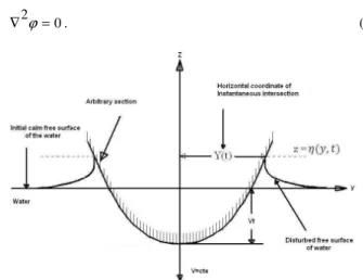
A two dimensional impact problem of a rigid body at a constant vertical velocity with an initially calm horizontal water surface is considered. The solid body is assumed to be symmetrical about its axis. In the assumed Cartesian coordinate system (y, z), y-axis lies
on the undisturbed water surface, while the z-axis coincides with the symmetric axis of the body (Fig. 1).
To illustrate the body surface, the relation h = H(y) is presented where h denotes the vertical distance between a point on the body surface and its apex. Water is considered to be incompressible and inviscid and flow to be irrotational. Here, the flow is described by a velocity potential ϕ that satisfies the Laplace’s equation with boundary condition in the fluid domain:
2 0
ϕ
∇ = . (1)
Figure 1. Two-dimensional body with arbitrary section dropping into (initially) calm water.
There are two free surface boundary conditions involved in the formulation of the problem:
(1) The kinematic boundary condition on the free surface:
D
Dt z
ϕ ∂ϕ =
∂ On z =η( , )y t (2)
(2) The dynamic boundary condition on the free surface: 1 2 2
( ) 0
2
D
g
y z
Dt ϕ
ϕ ϕ η
− + + = On z =η( , )y t (3)
where
D
Dt denotes the substantial derivative, η represents the vertical
coordinate of a point on the water free surface and g is the gravitational acceleration. The effect of possible air trapped between the body and the free surface is ignored and the effect of gravity compared to the body’s inertia can be considered negligible. Consequently, the dynamic boundary condition transforms into Eq. (4).
1 2 2 ( ) 0 2
D
y z
Dt ϕ
ϕ ϕ
− + = On z =η( , )y t . (4)
Nonlinear terms in these two boundary conditions are the sources of major difficulty in solving the boundary value problem. Therefore, to overcome this difficulty, Wagner (1932) simplified the dynamic boundary condition as:
( , , )y z t 0
( , )
z =η y t , which basically means that this condition must apply to the horizontal plane passing through the intersection points
( , )
z =η y t , and that the horizontal line is not the exact free surface. To determine the intersection point between the free surface and the body, the kinematic free surface boundary condition is used.
Another boundary condition is the no-flux condition which is imposed on the body surface:
V nz n ϕ ∂
= −
∂ On So( )t (6)
where n is the unit outward normal of the body surface, V is water entry velocity and So( )t represents the instantaneous wetted body surface. To determine So( )t , the relation h=H y( ) must be known with y ≤Y t( ) , where Y t( ) is the horizontal coordinate of the intersection point of the body and the free surface. Another boundary condition is the far field condition as in
0
ϕ
∇ → As (y2+z2 1/2) → ∞ . (7) For the initial condition, we can write:
( , , 0)y z 0
ϕ = & ( , 0)η y =0 on z =0. (8) Subsequent to finding the velocity potential ϕ, the pressure on the body is determined by Bernoulli equation and the impact force on the body is obtained by direct integration of the pressure over the wetted body surface.
The boundary value problem for ϕ must satisfy the Laplace’s equation, the kinematic free surface boundary condition, the linearized dynamic free surface boundary condition which is a Dirichlet boundary condition, the Newman body boundary condition, the radiation condition and the initial condition. It must be emphasized that the approximations carried out above are invalid for the flow region where the free surface profile changes sharply. However, for flow near the water intersection point, nonlinearity must be considered.
Analytical solution of boundary value problem
An analytical method for the solution of the linearized water entry problem of circular cylinder will be presented. To solve the Laplace’s equation, Eqs. (2), (5), (6) and (7) are implemented, which are known as boundary value problem for the velocity potentialϕ. It must be emphasized that the approximations made here are invalid for the flow region where the free surface profile changes sharply. The body boundary condition is imposed at the instantaneous position of the body. Since the Dirichlet boundary condition ϕ =0 is applied on the free surface z =η( )y , ϕ is considered symmetric with respect to z =η( )y plane. Therefore, the hydrodynamic images method can be used. As a result, the linearized boundary value problem can be considered as a closed body moving in an infinite fluid with a constant downward velocity,
V. This fictitious closed body is made of the immersed segment of the real body and its image about the horizontal plane z =η( )y . Therefore, the geometry of this shape depends on Y t( ). It should be noted that the position of the intersection of the body and the free surface, Y t( ), is a priori unknown, which must simultaneously be
solved with the initial boundary value problem. Thus, the velocity potential ϕ is a function of ( )Y t .
When the image method is used, the Galilean transformation can be utilized. Accordingly, we have:
( , , )y z t ( ', ', )y z t V z'
ϕ =ϕ − (9) where ϕ is the velocity potential for uniform flow passing a closed body, and relations between the (y', z') coordinate system and (y, z) coordinate system are:
' , ' ( )
y = y z = −z η y (10) To solve for ϕ analytically, the conformal mapping technique is applied, which depends on the body geometry. The best conformal mapping technique that may be used is Schwartz-Christoffel transformation.
Following the work done by Wagner (1932) and Mei et al. (1999), we define the intersection point ( ( ),Y t H Y( )−V t) as the location where the fluid particle on the free surface meets the body surface for the first time. Due to the usage of the kinematic free surface boundary condition and this definition, the governing equation for the intersection point y =l t( ) is taken to be:
( ) ( , ) 0
t
H l −V t = ∫v l τ τd (11)
where τ is the dummy time variable and ( , )v l τ is the vertical velocity of the fluid particle at y =Y t( ). Upon using Eq. (9), we have:
' ' '
( ,Y z ( ( )), )Y (Y Y t( ),z 0, )t V z
ϕ =η τ τ =ϕ = = − (12) Then, we write
( , ) ( , ( ), ) '( , 0, )
v l l Y l V
z z
ϕ ϕ
τ = ∂ η τ = ∂ τ −
∂ ∂ . (13)
Substitution of Eq. (13) into Eq. (11) would yield in
( ) '( , 0, ) 0
t
H Y l d
z ϕ
τ τ ∂
= ∫
∂ . (14)
By introducing the variable ( )Y vd dY
τ
µ = into Eq. (14) and changing the variable of integration from τ to Y, we will have
( ) 1
( ) ( , 0, ) ( ) 0 '
Y t
H Y v l Y dY
z ϕ
τ µ ∂
− = ∫
∂ (15)
If 0( , ) 1 ( , 0, ) '
v l Y v l
z ϕ
τ ∂ − =
∂ , Eq. (15) becomes
( ) 0( , ) ( ) 0
l
In order to perform the integration, the dependence of the kernel 0v on Y ( )η =l must be known. For arbitrary bodies, the dependence of 0v on l is complicated and a closed-form solution for µ( )l from Eq. (16) cannot be obtained. For bodies with smooth surfaces, the intersection point moves smoothly with time and hence varies smoothly with l. In such cases, we can write an expansion for µ( )l based on Chebyshev polynomial. The polynomial expansion of Chebyshev is applied to the first N terms to describe ( )µY as follows:
1 1
0 0
( ) ( )
N N
n
n n n
n n
Y a T Y b Y
µ − −
= =
=
∑
=∑
[0, ] maxY ∈ Y (17)
where an are the unknown coefficients, Tn represents the n-th order
Chebyshev polynomial of the first kind, Ymax is the maximum horizontal coordinate of the intersection point in the impact and bn is
0
n bn a ck kn
k
∑
=
= n=0,1, 2, ...,N (18)
where ckn are the known coefficients of the Chebyshev polynomial
Tn (Y ). To determine the unknown coefficients an, Eq. (17) is
substituted into Eq. (16) as in 1
( ) 0 ( ) 0
0
l N
H l v a Tn nY dY n
−
∑
= ∫
= . (19)
If the influence coefficient βn (Y ) is introduced as
( ) 0( , ) ( ) 0
l
l v l y T Y dY
n n
β = ∫ n=0,1, 2, ...,N −1 (20)
then, Eq. (19) becomes 1 ( ) ( )
0
N
H l an n l
n β
−
∑
=
= (21)
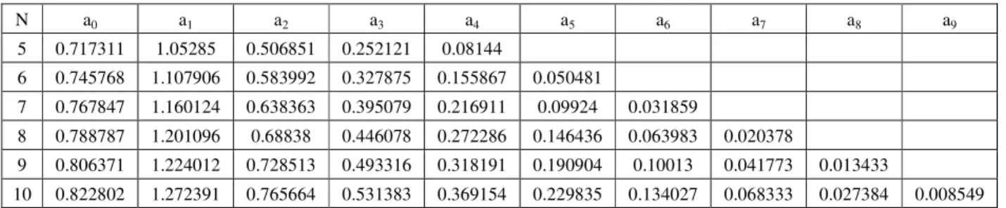
In the case of a circular cylinder, Eq. (21) must be determined numerically. By applying this equation at N + 1 discrete points on the body surface, a linear system of equation is formed. The resulting system of equation must be solved for an where n = 0, 1, … N. N can be chosen to be 10, in order to acquire a better accuracy for a circular cylinder (Table 1). In the next section, the water impact of a circular cylinder will be analyzed.
Table 1. Coefficients an for the circular cylinder section.
N a0 a1 a2 a3 a4 a5 a6 a7 a8 a9
5 0.717311 1.05285 0.506851 0.252121 0.08144
6 0.745768 1.107906 0.583992 0.327875 0.155867 0.050481
7 0.767847 1.160124 0.638363 0.395079 0.216911 0.09924 0.031859
8 0.788787 1.201096 0.68838 0.446078 0.272286 0.146436 0.063983 0.020378
9 0.806371 1.224012 0.728513 0.493316 0.318191 0.190904 0.10013 0.041773 0.013433
10 0.822802 1.272391 0.765664 0.531383 0.369154 0.229835 0.134027 0.068333 0.027384 0.008549
Impact of the circular cylinder
Consider the circular cylinder with radius R. All lengths are normalized with respect to the radius and then R = 1. The lower part of the circle can be defined by h l( )= −1 1−l2. As shown in Fig. 2, Y t( ) is the horizontal coordinate of the intersection point between the body and the free surface.
Figure 2. Definition of the horizontal coordinate of intersection point between the body and free surface.
The boundary condition ϕ =0 is applied on z =η( )y . This implies that the problem is equivalent to the solution of closed body,
which moves by constant velocity in the opposite direction of z-axis. The closed body is obtained by imaging the immersed part of body toward the z =η( )y or z' =0. Therefore, the velocity potential
' ' (y ,z , )t
ϕ at any instant t describes the vertical uniform flow past (doubly convex) lens of width 2Y(t) and thickness 2h(Y). Finally, closed form solution for ϕ can be obtained by conformal mapping. The physical flow in the Z-plane is mapped onto a uniform vertical stream in the W-plane through a double conformal mapping:
tan
iY Z
Q − = ,
sin( )
iY v W
vQ −
= (22)
where Q = +ξ iζ is as intermediate complex variable and dimensionless coefficient
v
which is defined as/ 2 2 ( / (1 (1 ) )
v
arctan Y Y
π =
− −
. (23)
Figure 3. Definition of the planes W, Z and Q.
Therefore, the velocity potential can be obtained as ' '
(y ,z , )t Re{ iV W}
ϕ = − (24) where Re means the real part of the expression and the vertical component of the velocity vector may be acquired by the following computations:
2 cot( ) sin( )
dW iY v vQ
dQ vQ
= ,
2 sin
dQ Q
dZ = iY
2 2 2 2
sin ( ) sin ( ) '
' sin( ) tan( ) sin( ) tan( )
dW v Q i v Q
V z
dz vQ vQ vQ vQ
ϕ
→ = ⇒ = .
Thus, the complex velocity is 2 2 sin sin( ) tan( )
v Q
u iv iV
vQ vQ
− = − (25)
The variable V0( , )y l at the free surface position and at the '
1
Z = y = →Q =iζ can be achieved as 2 2 ( , 0, ) sin 1
( , )
0 ' sin( ) tan( ) 2sinh2
sinh( ) tanh( )
l v Q
V y l V
vQ vQ z v v v ϕ τ ζ ζ ζ ∂ − = = ∂ =
. (26)
The variables ζ and l are related by
tan( ) tan( ) 1
tanh( )
iY iY
Z l
iQ i
l e e
Y e e
ζ ζ ζ ζ ζ ζ = − → = − → − + = − = − − − 1 2 2
( 1) ( 1) ln( ) 2
l l Y
e e
Y l Y
ζ ζ ζ −
→ − = − + → =
+ . (27)
The velocity potential is a function of the intersection point between the body and the free surface. The velocity potential can be calculated by solving the boundary value problem, but the intersection point is an unknown which must be obtained.
To determine the unknown value an, the influence coefficient
βn (l ) must be determined. By substituting Eq. (26) into Eq. (20),
we have
2 2 1 sinh ( )
( )
0 sinh( ) tanh( ) for 0,1, 2, ..., 1
v TnY
l dY n v v n N ζ β ζ ζ = ∫ = −
. (28)
Due to the intricacy of the dependence of v and ζ upon l, the above equation may not be evaluated analytically. Therefore, Eq. (28) must be evaluated numerically for a given value of Ymax/R. Equation (21) must be evaluated at N discrete points. To achieve fast convergence, the discrete points must be the extremum of the coefficient of the Chebyshev polynomial. The coefficients an for different value of n are given in Table 1. It is seen that by increasing n, the coefficients an will have no effect.
The present analytical solution can be employed at the very initial time of the impact. In this situation, in order to solve Eq. (28), an asymptotic solution can be obtained. When V t <<1, the intersection point will be Y <<1. Therefore, by using Taylor expansion and very small values of l (l <<1), the circular cylinder may be represented as
2 4 ( ) ( )
2
l
h l = +O l . Based on Eq. (23), we have v = +1 O Y( ). This can lead to
( , ) cosh( )
0 2 2
2
l Y l Y
l
l Y l Y
v l Y
l Y ζ − + + + − = = = −
. (29)
Finally, we can arrive at 1 1
( ) [1 ( )]
2 0 0 1
k
n k
l l c d O l
n k kn
λ β λ λ + ∑ = ∫ +
= − (30)
which represents the influence coefficient, as pointed out earlier.
Pressure distribution and slamming force
After obtaining the motion of the intersection point, the boundary value solution can now be obtained and substituted in Eq. (24), in order to determine the velocity potential ϕ. By determining the velocity potential ϕ, the pressure at any wetted part of the body surface can be evaluated using the Bernoulli's equation, which in terms of the velocity potential ϕ can be expressed as
( , ) 1 2 2 ( ) 2
P l t
y z t ϕ ϕ ϕ ρ ∂ = − − + ∂
( , ) 1 2 2 ( ) 2
P l t D
v z y z
Dt ϕ
ϕ ϕ ϕ
ρ
→ = − − − + (31)
( , , )y z t '( ', ', )y z t v
z z
ϕ =ϕ − (32) and
' ( )
D D Dz D DH Y
v v
Dt Dt Dt Dt Dt
ϕ φ φ
= − = + . (33)
Hence, after substituting (33) and (32) into (31), the pressure can be written in terms of ϕ (the velocity potential for the uniform flow passing a closed body) as
( , ) 1 2 1 2 2 ( ) ( ' ')
2 2
P l t D DH Y
v y z v
Dt Dt
ϕ
ϕ ϕ
ρ = − + − + − . (34)
Details of the relation may be found in Mei et al. (1999).
Numerical Method
Governing equations
The governing equations for the fluid flow are momentum and continuity, which are as follows:
2 1
ui ui p ui
ui gj
t xj xi xj xj
ν ρ
∂ ∂ ∂ ∂
+ = − + +
∂ ∂ ∂ ∂ ∂ (35)
0
ui x i ∂
=
∂ (36)
In order to capture the sharp interface in hydrodynamic two-phase flow problems, the volume of fluid method is employed. The VOF technique uses a color function named Volume Fraction (α). A transport equation (37) is then solved for the advection of this scalar, using the velocity field calculated from the solution of the Navier-Stokes equations at the last time step.
.( u) 0
t α
α ∂
+ ∇ =
∂
r r
(37)
Numerical solution of Eq. (37) gives the volume fraction of each phase (i.e. Air and Water) in all computational cells. Distribution of the volume fraction (α) is as follows:
1 for cells including fluid 1 0 for cells including fluid 2 0 1 for cells including the interface
α
α =
< <
(38)
Using the volume fraction, an effective fluid with the variable physical properties is introduced:
(1 )
1 2
(1 )
1 2
eff
eff
ρ αρ α ρ
υ αυ α υ
= + −
= + − (39)
where subscripts 1 and 2 represent two phases, e.g. Water and Air. For rigid body motion simulation, a body fitted mesh is used which will follow the body motion over time. This strategy is called the moving grid technique in which the grid velocity will be integrated into the surface fluxes calculated on each control volume face.
The confluence of boundary condition can cause singularities in the free surface displacement and velocities, as anticipated by the linear theory. These singularities appear to be avoided in the real fluid by the formation of jets which quickly break up into sprays under the action of surface tension. Therefore, for including nonlinearity effect in the water impact problem of a circular cylinder, a commercial VOF solver, i.e. FLOW-3D (FLOW-3D Manual, 2009), is employed. The FLOW-3D code applies the FVM (finite volume method) in combination with the volume of fluid solution for free surface flow. VOF is an excellent tool for the simulation of two phase flow which includes water and air in this study. In this numerical scheme, an additional transport equation is solved for the volume percentage of air in each cell. More details of FVM and VOF solution can be found in many reference books and articles (Versteeg and Malalasekera (1995), Jasak (1996), Kleefsman et al. (2005), Rhee et al. (2005), Sicilian (1990), Hirt (2004), and Barkhudarov (2004)).
A circular cylinder of arbitrary radius R and constant falling velocity is considered. The computational domain considered is a semi-circular lower region with radius 8 times larger than the body, and an upper rectangular region extending 3 times the radius of the body, as shown in Fig. 4.
Figure 4. Computational domain and structured grid.
Results and Comparisons
The vertical water entry of a two-dimensional circular cylinder at constant velocity is computed using both linear analytical solution and fully nonlinear numerical method. Various aspects of water impact of circular section are studied and linear and nonlinear solutions are compared with each other and against the results of previous works. Pressure coefficient (CP), impact force coefficient
(CS), free surface profile, contours of pressure and evolution of the
intersection point are presented with special considerations given to the motion of the intersection point.
Based on Eqs. (22)-(25) and Eq. (34), the pressure distribution on the wetted body surface can be derived analytically. The obtained analytical expression for pressure should be evaluated numerically to gain the pressure distribution on the wetted part of the body surface. Figure 5 shows the pressure distribution at different time instants during the impact, based on both analytical results and numerical solution. It can be seen that the maximum pressure is initially located near the intersection point and eventually moves to the keel point.
For validation, the impact force on the cylinder which is directly related with pressure distribution is compared against the experimental results of Campbell and Weynberg (1980) and potential flow results based on a finite difference method (Arai, 1995). In the experiment, the cylinder is forced into the water with constant velocities. The comparisons are shown in Fig. 6. The present predictions based on analytical solution lie closer to the experimental results, but the best agreement is achieved by the current numerical findings which agree very well with the experiments. The three-dimensional effects in the experiments produce this small inconsistency.
Figure 5. Pressure distribution at different time instants during the impact.
Figure 6. Impact force on a circular cylinder entering the water with constant velocity.
Figure 7. Free surface profile at four different time instants: a) t = 0.01, b) t = 0.05, c) t = 0.1 and d) t = 0.15.
Figure 8. Contours of pressure at four different time instants: a) t = 0.01, b) t = 0.05, c) t = 0.1 and d) t = 0.15.
Snapshots of four configurations at different stages of the penetration are illustrated in Fig. 7. The corresponding pressure contours are also presented in Fig. 8.
From Fig. 5, it is obviously clear that the pressure peak gradually decreases and its effective area increases. Figure 8 shows that the maximum pressure gradient and maximum pressure appear at the spray root. This remains so until the spray detaches.
The obtained free-surface profiles show that the thickness of the jet grows with the local deadrise angle of the impacting body and that, due to the rise up of the water, the wetted part of the cylinder is larger than the penetration measured at the still water level. The numerical simulation is in fact quite similar to that of Greenhow (1988). But all these are not the main concern here, as the purpose of this paper is to provide some understanding about the movement and characteristic of the flow near the intersection point and a comparison between linear and nonlinear solutions. This information can contribute to the physical understanding of the problem, which in turn can play an important role in the development of the numerical codes.
solution provides much higher speed for motion of the intersection point compared to the results of the two models offered here.
Figure 9. Evolution of the intersection points.
In the problem considered, based on the linear theory, the assumption of the linear free surface boundary condition leads to an unrealistic conclusion that the displacement of liquid particles at the intersection points are unbounded. This implies that the assumption is not valid near the intersection points, where separation of the liquid particles from the cylinder surface occurs. The position of the separation points have to be determined together with the liquid flow and the pressure distribution.
The obtained free surface profile using the VOF solver confirms that the liquid flow near the intersection points is different from that in the main region. Thus, separation effects as well as the gravity must be taken into account. Liquid particles on the body surface, which are initially close to the separation points, can leave the body surface after the motion starts.
Conclusion
The present study focuses on the derivation of analytical formulas for a water entry problem and conducts a comparison between the linear and nonlinear solutions. Accordingly, a numerical solution is also obtained by the FLOW-3D software, a commercial VOF solver. Some attention is also given to the point of intersection between the free surface and the body, where the confluence of boundary condition can cause singularities in the free surface deformation and velocities, as predicted by the linear theory. These singularities appear to be avoided in the real fluid by the formation of jets which quickly break up into sprays under the action of surface tension. It is also understood that the gravity is of major importance near the intersection point. Pressure distribution, slamming force, free surface profile, contours of pressure and the evolution of intersection point are presented. By comparisons between analytical solutions, numerical results and existing previous studies, one can conclude that the numerical findings are more favorable, which is consistent with the expectation that a fully nonlinear model should behave in such a way. On the other hand, a less complicated analytical solution has also shown to be relatively close to the experimental results which may become very useful in some practical situations. Numerical investigation of general bow section may be considered as a future study.
References
Arai, M., Cheng, L.Y., Inoue, Y., and Miyauchi, T., 1995, “Numerical study of water impact loads on catamarans with asymmetric hulls”, in Proc. FAST’95, Travemünde.
Armand, J.L., Cointe, R., 1987, “Hydrodynamic impact analysis of a cylinder”. Proc. Fifth Int. Offshore Mech. and Arctic Engng. Symp., Tokyo, Japan, pp. 609-634.
Barkhudarov, M.R., 2004, “Lagrangian VOF Advection Method for FLOW-3D”, FSI-03-TN63-R.
Campbell, IMC., Weynberg, PA., 1980, “Measurement of parameters affecting slamming”, Final Report, Rep. No. 440, Technology Reports Center No. OT-R-8042. Southampton Univeristy, Wolfson Unit for Marine Technology.
Faltinsen, O.M., 1990, “Sea loads on ships and offshore structures”, Cambridge: Cambridge University Press.
Faltinsen, O.M., Kjærland, O., Nottveit, A., Vinje, T., 1977, “Water impact loads and dynamic response of horizontal circular cylinders in offshore structures”, In: Proc. 9th annual offshore technology conference, Vol. I, pp. 119-25.
Greenhow, M., 1988, “Water-entry and -exit of a horizontal circular cylinder”, Journal of Applied Ocean Research, Vol. 10, pp. 191-8.
Hirt, C.W., 2004, “Modeling Turbulent Entrainment of Air at a Free Surface”, FSI-03-TN61.
Howison, S.D., Ockendon, J.R., Wilson, S.K., 1991, “Incompressible water-entry problems at small deadrise angles”, Journal of Fluid Mechanics, Vol. 222, pp. 215-230.
Jasak, H., “Error analysis and estimation for finite volume method with application to fluid flows”, Ph.D. Thesis., University of London, 1996.
K.M.T. Kleefsman, G. Fekken, A.E.P Veldman, B. Iwanowski, and B. Buchner, A, 2005, “Volume-of-Fluid based simulation method for wave impact problems”, J. Comput. Phys., 206, pp. 363-393.
Korobkin, A., 2004, “Analytical models of water impact”, European Journal of Applied Mathematics, Vol. 15, pp. 821-838.
Logvinovich, G.V., 1969, “Hydrodynamics of Flows with Free Boundaries”, Naukova Dumka.
Mei, X., Liu, Y., Yue, D.K.P., 1999, “On the water impact of general two-dimensional sections”, Journal of Applied Ocean Research, Vol. 21, pp. 1-15.
Oliver, J.M., 2002, “Water entry and related problems”, PhD thesis, University of Oxford.
Rhee, S.H, Makarov, B., Krishinan, H., Ivanov, V., 2005, “Assessment of the volume of fluid method for free surface wave flow”, J. Mar. Sci. Technol., 10, pp. 173-180.
Sicilian, J., 1990, “A ‘FAVOR’ Based Moving Obstacle Treatment For Flow-3D”, FSI-90-00-TN24.
Sun, H., Faltinsen, O.M., 2006, “Water impact of horizontal circular cylinders and cylindrical shells”, Journal of Applied Ocean Research, Vol. 28, pp. 299-311.
Versteeg, H.K., Malalasekera, W., “An introduction to computational fluid dynamics: the finite volume method”, Wiley Publication, 1995.
Von Karman, T., 1929, “The impact on seaplane float during landing”, NACA TN321.
Vorus, W.S., 1996, “A flat cylinder theory for vessel impact and steady planing resistance”, Journal of Ship Research, Vol. 40, pp. 89-106.
Wagner, H., 1932, “Über Stoß- und Gleitvorgänge an der Oberfläche von Flüssigkeiten”, ZAMM,12, pp. 193-215.
Xu, L., 1998, “A theory for asymmetric vessel impact and steady planning”, PhD thesis, University of Michigan.
Zhao, R., Faltinsen, O., Aarsnes, J., 1996, “Water entry of arbitrary two-dimensional sections with and without separation”, Proc. 21st Symposium on Naval Hydrodynamics, Trondheim, Norway, pp. 118-133.