Indirect Identification of the Complex Poisson's Ratio in Fractional Viscoelasticity

(1)

Indirect Identification of the Complex Poisson's Ratio in Fractional

Viscoelasticity

Abstract

The use of viscoelastic materials (VEMs) has becoming more and more fre-quent both as vibration control in general or as parts of structural components. In all applications, the mechanical behavior of such materials can be predicted by the complex moduli (Young’s, shear or volumetric) and the complex Pois-son’s ratio. Over recent decades, various methodologies have been presented aiming at characterizing complex moduli. On the other hand, the indirect identi-fication of the Poisson’s ratio, in the frequency domain, proves to be underex-plored. The present paper discusses two computational methodologies in order to obtain, indirectly, the complex Poisson’s ratio in linear and thermorheologi-cally simple solid VEMs. The first of them uses a traditional methodology, which individually identifies the complex Young’s and the shear moduli and, from them, one obtains the complex Poisson’s ratio. The second methodology – proposed in the present paper and called ‘integrated’ – obtains the complex Poisson’s ratio through a simultaneous identification of those two complex moduli. Both methodologies start from a set of experimental points of the com-plex moduli in the frequency domain, carried out at different temperatures. From those points, a hybrid optimization technique is applied (Genetic Algo-rithms and Non-Linear Programming) in order to obtain the parameters of the constitutive models for the VEM under analysis. For the experiments described here, the integrated methodology proves to be very promising and with a great application potential.

Keywords

Viscoelastic behavior; Complex Poisson's ratio; Complex Young's modulus; Complex shear modulus; Hybrid optimization.

1 INTRODUCTION

In engineering, viscoelastic materials (VEMs) are used not only in vibration and noise control but also as structural components (Nashif et al., 1985; Pacheco et al., 2014; Ribeiro et al., 2015). In both cases, in bidimensional (or tridimen-sional) stress-strain analysis, it's necessary the knowledge of the complex moduli (shear, Young and volumetric) and the complex Poisson's ratio of the material (Benedetto et al, 2007; Allou et al., 2015).

In perfectly incompressible materials, the value of the dynamic Poisson's ratio tends to 0.5. In general, elastomers are treated as almost incompressible materials with values of this parameter assumed to be constant and slightly less than 0.5 (Sim and Kim, 1990; Espíndola et al., 2005; Hecht et al., 2015). It is notable that such considerations ignore time and frequency effects. However, in practice, this parameter is variable in frequency, as well as in time (Pritz, 1998; Pritz, 2000; Tschoegl et al., 2002; Pritz, 2007; Chen et al., 2017).

The identification of the complex Poisson’s ratio in the frequency domain can be performed through direct or indi-rect methods (Pritz, 1998; Tschoegl et al., 2002). In diindi-rect methods, the ratio can be obtained from measurements per-formed directly on the structure (Kabeer et al. 2013; Cui et al. 2016). On the other hand, in indirect methods, the identifi-cation occurs by constructing and evaluating auxiliary complex viscoelastic functions (Young's, shear and/or bulk modu-lus). The present work focuses on the indirect method, which has been little explored by researchers in recent decades (Philippoff and Brodnyan, 1955; Koppelman, 1959; Thomson, 1966; Waterman, 1977; Pritz,1998; Pritz, 2000; Pritz, 2007; Chen et al., 2017).

Tiago Lima de Sousaa * Jéderson da Silvaa,b Jucélio Tomás Pereiraa a

Programa de Pós-graduação em Engenharia Mecânica, Universidade Federal do Paraná - UFPR, Curitiba, Paraná, Brasil. E-mail:

tiago.sousa.eng@gmail.com, jucelio.tomas@ufpr.br

b_{Departamento de Engenharia Mecânica,}

Universidade Tecnológica Federal do Paraná - UTFPR, Londrina, Paraná, Brasil. E-mail: dasilva.jederson@gmail.com

*Corresponding author

http://dx.doi.org/10.1590/1679-78254920

(2)

One of the pioneering works on this issue is present by Philippoff and Brodnyan (1955), which obtains the Pois-son’s ratio, firstly, through the complex Young’s and the shear moduli and, subsequently, through the complex Young’s and bulk moduli. As a result, different functions are obtained for the Poisson’s ratio.

Koppelman (1959) carries out experiments in the frequency domain, varying between ₁₀5_and₁₀1_Hz, consider-ing the influence of temperature, which varies from 20°C to 100°C, for both the complex Young’s modulus and the complex shear modulus. This temperature range corresponds to the glassy region of the material (polymethyl methacry-late). In the experiments, the absolute Poisson’s ratio is around the average value of 0.31, independently of either fre-quency or temperature. However, no analysis is carried out in the rubbery region, which makes it difficult to identify the complex Poisson’s ratio properly.

Later on, Thomson (1966) uses experimental data from the literature for the complex moduli (Young’s and shear) and carries out a point-by-point calculation of the complex Poisson’s ratio, the real part of which is a non-monotonic function in the frequency domain. However, Theocaris (1968), Waterman (1977) and Pritz (1998) mathematically show - together with experimental evidences - that the real part of the complex Poisson’s ratio is monotonically decreasing, the loss factor has at least one maximum with respect to frequency, and the imaginary part has strong evidence of being negative, regarding polymeric materials.

Pritz (2000) suggests that the most effective method for determining the complex Poisson’s ratio modulus - using the indirect method and a wide frequency range - is by measuring the complex bulk and shear moduli. Pritz (2007) car-ries out a theoretical and experimental study of the Poisson’s loss factor for linear VEMs. As a result, it has been found that the Poisson’s loss factor is approximately proportional to the difference between the shear and bulk loss factors. In addition, it is shown that the Poisson’s loss factor is smaller than the shear loss factor usually by one order of magnitude at least.

Recently, Chen et al. (2017) have obtained experimental data for dynamic moduli in traction and shear and, through Prony’s fractional viscoelastic model, they have obtained the functions for Poisson’s ratio and the bulk modulus. An important premise in the present work is the fact of considering the bulk modulus as constant.

From this brief review of literature, one notices that some methodologies face difficulties in identifying indirectly the viscoelastic function of the complex Poisson’s ratio. Some papers suggest that it should be obtained through the shear and bulk moduli. However, obtaining the complex bulk modulus requires high costs and complex apparatus (Fillers and Tschoegl, 1977; Tschoegl et al., 2002; Emri and Prodan, 2006). Other methodologies suggest that the bulk modulus stays constant, which, in practice, according to Tschoegl (1989), Pritz (1998), and Emri and Prodan (2006), proves to be varia-ble. It is important to note that all mentioned methodologies seek to identify VEMs with linear and thermorheologically simple behaviors.

Additionally, the mathematical modeling of the mechanical behavior of VEMs can be described through rheological models involving integer or fractional order derivatives. According to Pritz (1998), Espíndola et al. (2005), Mainardi (2010) and Ribeiro et al. (2015), the fractional models are powerful tools in projects involving vibration control, in par-ticular the fractional Zener model. The advantage of such models is not only their ability to describe actual dynamic behavior, but also that they are causal and simple enough for engineering calculations. In addition, the fractional Zener model can be used to describe the variations of dynamic properties over a wide range of frequency and temperature, since that the loss factor has a single peak (Pritz, 2003; Sousa et al. 2017).

In this context, the aim of the present work is to develop and apply a numerical and integrated methodology to ob-tain, indirectly, the complex Poisson’s ratio of linear and thermorelogically simple VEMs. Such methodology is based on the reading of a set of experimental points of the complex Young’s and shear moduli in the frequency domain and at different temperatures. Based on those points, a hybrid optimization technique is applied using Genetic Algorithms (GA) and Non-Linear Programming (NLP) to obtain the parameters of the constitutive model, i.e. fractional Zener model, for the VEM in present study. Lastly, relating the identified complex moduli (Young’s and shear) the complex Poisson’s ratio and the complex bulk modulus are obtained.

2 THEORETICAL CONCEPTS

(3)

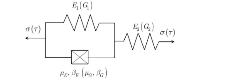
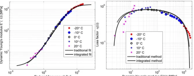
According to Mainardi (2010), an improvement on the classical models of linear viscoelasticity may occur when re-placing Newton’s viscous dampers by Scott-Blair’s fractional dampers. Thus, the mechanical model differential equa-tion, written in terms of integer order derivatives, is replaced by an equation involving fractional derivatives. According to Glöckle and Nonnenmacher (1994), Galucio et al. (2004), Mainardi (2010), Rouleau et al. (2015) and Ciniello et al. (2016), there are several constitutive models involving fractional order derivatives: Maxwell, Kelvin-Voigt, Zener etc.. As presented by Mainardi and Spada (2011) and Ciniello et al. (2016), the Zener fractional model (Figure 1) proves to be fairly efficient in predicting the behavior of linear VEMs.

Bagley and Torvik (1986), Galucio et al. (2004) and Mainardi (2010) show that the fractional order differential equation that governs the fractional Zener physical system (Figure 1) may be written as

0 0

1 E E ( ) E E ( ),

E E

E E E

d d

t E E r t

dt dt            _  _  _  _   _   _  __  __  

    (1)

where ( )t and ( )t are stress and strain history, respectively. The equation parameters are related with Zener

rheological model as E₀  E E₁ ₂ / (E₁  E₂), r_E  (E₁  E₂) /E₁ and E / ( ₁ ₂)

E E E E

   . Where,

E

₁ and

E

₂

are stiffness moduli of the elastic elements, dE dtE() represents a differential operator of fractional order



_E and



_E

is the viscosity ratio of the Scott-Blair's damper (Mainardi, 2010). It is important to note that, in the International System of Units (SI), the variables

E

₀,

E

₁ and

E

₂ have units MPa,



_E and



_E have units, respectively, s and sE MPa, and

E

r

is dimensionless.

In the present study, the Riemann-Liouville definitions (Mainardi, 2010), for the fractional derivative, are the most appropriate, since it is considered that the structural system is initially at rest and there is no need to treat the information that occurs for a time

t



0

. Thus, considering a function

f t

 

, the definition of the Riemann-Liouville fractional de-rivative on the left, with differentiation order of , is given as

 

_{ }







 



0 ₀ 1 , 1 m _t t _m

d f t d f

D f t d m m

m t dt dt            _ _    

 



 (2)

where  is a positive real number, m is a positive integer number and

 

 

is the Euler's Gamma function (Li and Zeng, 2015). In this case, according to Mainardi (2010) and Kazem (2013), the Laplace transform for the Riemann-Liouville fractional derivative of order , can be placed as

 



0 t



 

.

L D f t _  _ s f s (3)

In such a way, according to Tschoegl (1989), Mainardi (2010) applying Laplace transform to all terms of Eq. (1), for t > 0, considering a steady state sinusoidal excitation of axial frequency, the steady-state response may be written as



_{( )}

( )

0

_,

( )

₁

E

E b s

s

E s

s

_{b s}

 













(4)

where E

E E

b  ,

E

_



E r

₀_E and

E s



 

is defined as Young’s operational modulus (Tschoegl, 1989; Rahman and

Tarefder, 2016). In SI, the units of

b

_E and

E

_ are, respectively, s _and

_MPa

_{. In general, during the identification of}

(4)

Figure 1: Fractional Zener rheological model. The parameters on this illustration are related to uniaxial and shear testing.

Note that Eq. (1) is written in terms of a uniaxial tension testing. Such equation has a corresponding form that re-lates history of stress, ( )t , and strains, ( )t , in pure shear tests. Therefore, according to Mainardi (2010), Pritz (2003)

and Ciniello et al. (2016), following a similar reasoning, the shear operational modulus,

G s



 

, can be presented as

0

( )

,

( )

₁

G

G b s

s

G s

s

_{b s}

 















₍₅₎

where G / ( ₁ ₂)

G G G

b   G G ,

G

₀



GG

_{1 2}

/(G

₁



G

₂

)

,

G

_



Gr

₀_G and

r

_G



(

G

₁



G

₂

)/

G

₁. In this case,

G

₁

and

G

₂ are the stiffness moduli of the elastic elements,



_G is the viscosity ratio, and



_G, with

0 



_G



1

, is the

fractional-order of Scott-Blair shock absorber (see Figure 1). Analogously, in SI, the variables

G

₀,

G

_,

G

₁,

G

₂, have

units MPa,



_G,



_G and

b

_G have units s_,sG MPa and s, respectively, and

r

_G is dimensionless.

According to Tschoegl (1989) and Park and Schapery (1999), the complex viscoelastic functions arise from the re-sponse to a steady-state sinusoidal loading, and are related to the operational functions as follows

*_{( )} _{( )} *_{( )} _{( )} _,

s i s i

E  E s _{ } and G  G s _{ } (6)

where

E

*

( )



and

G

*

( )



are the complex Young’s modulus and the complex shear modulus, respectively. This way, Eqs. (4) e (5) may be rewritten as

 

0 0 *_{( )} *_{( )} _. 1 1 G E E G G E E G

G G b i E E b i

E and G

b i b i

                  (7)

These moduli have a real and an imaginary components, which can be placed as

 

*_{( )} _' _'' *_{( )} _' _'' _,

E  E  iE  and G  G  iG  (8)

which represent storage and loss of energy, respectively. In addition, the components

E

'

 



,

G

'

 



,

E

''

 



, and

 

''

G



are defined, respectively, as the dynamic Young’s modulus, the dynamic shear modulus, the loss Young’s modulus and the loss shear modulus. By relating the two complex moduli discussed, in the frequency domain, it is possible to obtain a third modulus, defined as complex bulk modulus,

K

*

 



, which can be presented as

 

   

 

* * * * *

'

''

,

9

3 E

G

K

iK

G

E



 

 

 

 



(9)

where

K

'

 



and

K

''

 



are defined, respectively, as the dynamic bulk modulus and loss bulk modulus (Tschoegl, 1989).

Given the initial definitions, the loss and storage moduli can be related as follows   1 1 E G   2 2 E G





, ,

E E G G

   

( )

 

( )

(5)

 

''

   

'

,

 

''

   

'

 

K''

   

K'

,

E

G

and

K



 





 





 



(10)

where



_E

 



,



_G

 



and



_K

 



are functions defined as ‘loss factors’ of the complex Young’s, shear and bulk moduli, respectively.

In addition, according to Nashif et al. (1985) and Tschoegl (1989), the complex Poisson’s ratio in the frequency domain,



*

 



, may be obtained relating the complex moduli of Eq. (8) as

 



 



* _E* ₂_G* _1.

      (11)

This way of obtaining the complex's Poisson ratio is called the indirect method which is based on the evaluation of auxiliary functions (complex Young’s and shear moduli). Another way of obtaining it is through the direct method, which is discussed in section 2.1.

2.1 COMPLEX POISSON'S RATIO

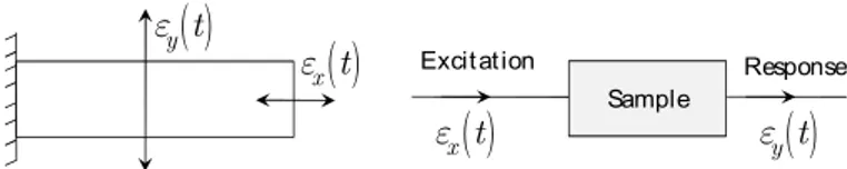
Physically, the complex Poisson's ratio is defined as the ratio of lateral strain to axial strain. Assuming application of a dynamic strain in the longitudinal direction, the lateral strain is delayed in relation to the axial strain due to the ener-gy dissipation capacity of the material (Theocaris, 1968; Kugler et al., 1990; Pritz, 1998; Cui et al., 2016). As a result, if the dynamic axial strain is a harmonic function, represented in the complex form according to

 

ˆ

i t x

t

x

e



_



 _, ₍₁₂₎

the lateral strain can be placed as

 

_ˆ i t 

y t ye 

     , (13)

where



ˆ

_x and

ˆ



_y are the strain amplitudes,



is the angle of delay of the lateral strain in relation to the applied axial strain (Tschoegl, 1989; Pritz, 2007; Graziani et al., 2014).

Figure 2: Illustration of measurement the Poisson's ratio by means of the direct method.

Therefore, the ratio of the lateral strain,



_y

 

t

, to the axial strain,



_x

 

t

, results in the complex Poisson’s ratio

 

*

   

*

 

* _y i _x i ' i '' ' 1 i _

              _    _, (14)

in which



_y*

 

i



and



_x*

 

i



are the Fourier transform of the lateral and axial strain functions in the time domain,

 

y

t



and



_x

 

t

, respectively,



'

 



is the dynamic Poisson’s ratio,



''

 



is the loss component. In this case, due to

the lateral strain delay, the imaginary component of this complex ratio is negative (Pritz, 1998). Furthermore,



_

 



is the loss factor obtained as

 

''

   

'





 









. (15)

The complex Poisson's ratio describes, in the frequency domain, ratio of the lateral strain to axial strain. So, if it's supposed that the complex Poisson's ratio can be interpreted as the frequency response function of a linear system, the system may be a material specimen as shown in Figure 2. Thereby, Booij e Thoone (1982), Pritz (1998), Pritz (2000), Pritz (2007) and Rouleau et al. (2015) demonstrate that the real and imaginary components of the complex Poisson's ratio are linked through the Kramers-Kronig relations as

Sample

Excitation Response

 

x t

 _y

 

t

 

x t



 

y t

(6)

 

'

 

log '

 

''

2 2 log

d d

and

d  d

 

 

           

 

  __ __ . (16)

It follows from Eq. (16) that the slope of the curve



'

 



is negative (



''

 

 

0

) (Theocaris, 1968; Tschoegl, 1989; Pritz, 2007). Thus, the dynamic Poisson's ratio of solid VEMs must decreases monotonically with increasing fre-quency.

The viscoelastic functions presented in this section constitute a basis from which it is possible to predict the behav-iors of linear and thermorheologically simple VEMs, in the frequency domain. In addition, by means of interconversions, one can obtain the corresponding viscoelastic functions in time domain.

2.2 COMPLEX MODULI CONSIDERING TEMPERATURE

In order to analyze the viscoelastic behavior of the material in the frequency domain and considering the influence of temperature, the complex moduli (Young's, shear and bulk), Eqs. (6) and (9), may be rewritten as function of a re-duced frequency,



_R, as (Jones 1974; Nashif et al., 1985; Pritz, 1996)





*_{( , )} *_{( ),} *_{( , )} *_{( )} * _, *_{( ),}

r r r

E T  E  G T  G  and K T  K  (17)

where



_r groups the temperature effects, T, and the frequency effects,



. This variable is represented by

.

r



T

 



(18)

Additionally,



_T is a function - defined as a shift factor - that describes the dependency of the VEMs relaxation times regarding temperature; and, in the present paper, it follows the Williams-Landel-Ferry (WLF) model (Williams et al., 1955) given by

1 0 2 0 ( ) log , ( ) T T _T

C T T

   

  (19)

where

C

₁T and

C

₂T are constants to be determined, which are related to the material properties; and

T

₀ represents the reference temperature (Ferry, 1980; Ward and Sweeney, 2004; Brinson and Brinson, 2008). Thus, considering the influence of temperature, the complex Young’s and shear moduli can be presented as

















0 0

*_{(T, )} *_{( , )} _.

1 1 G E E G G r E r

E r G r

G G b i E E b i

E and G T

b i b i

                  (20)

Analyzing the Eq. (20), it is noted that each complex modulus (Young's or shear) has six material properties, result-ing in a total of twelve material parameters for a VEM's complete characterization.

On the other hand, according to Ernst et al. (2003), Lakes and Winemam (2006), O’Brien et al. (2007), and Chen et al. (2017), the influence of temperature and the orders of differentiation are the same for both complex moduli (Young's or shear). In this case, the WLF constants can be obtained as T_,1= T_,1 T _{, 1}

E G EG

C C C and T_,2= T_,2 T _,2

E G EG

C C C .

Moreo-ver, that the order of differentiation can be simplified as

 



_E





_G. In view of such considerations, the complete identification of the VEM parameters is reduced to a total of nine material parameters.

3 EXPERIMENTAL DATA, METHODOLOGY, AND COMPUTATIONAL STRUCTURE

3.1 EXPERIMENTAL DATA

In the current work, the material under study is the EAR®

C-1002. This is a elastomeric polymer, known commer-cially as ISODAMP C-1002, manufactured by EAR®

(7)

VEMs (Espíndola et al., 2006; Nayfeh, 2004; Sousa et al. 2017). Jones (1992) takes a set of samples of this material and sends them to some laboratories in the world (named generically Laboratory A to Laboratory F). These laboratories have the mission to carry out experimental tests involving the complex moduli (Young and Shear) in frequency domain and considering the temperature effects.

Considering the experimental data analysis, the linear viscoelasticity theory (Ferry, 1980; Tschoegl, 1989; Mainardi 2010), and aiming at evaluating the identification methodology proposed here, the present paper uses the experimental data presented by laboratories C and E. Graphic representations of those experimental data are provided from Figure 3 to Figure 6.

From the available experiments, it is possible to identify the material using the fractional Zener model, either through the traditional method or through the proposed method, here referred to as the ‘integrated method’.

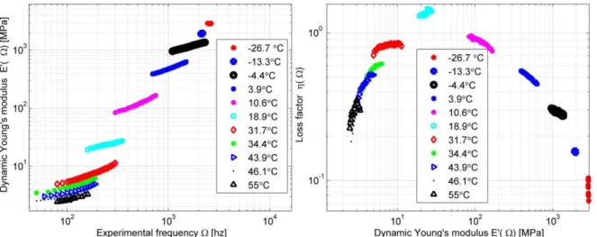
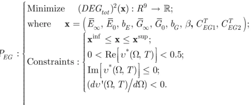
Figure 3: Lab C. Experimental data for complex Young's modulus: dynamic Young's modulus (left) and wicket plot (right).

(8)

Figure 5: Lab E. Experimental data for complex Young's modulus: dynamic Young's modulus (left) and wicket plot (right).

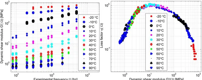
Figure 6: Lab E. Experimental data for complex shear modulus: dynamic shear modulus (left) and wicket plot (right).

3.2 METHODOLOGY

Given a set of experimental points, a standard optimization problem is constructed aiming at minimizing a function that represents a measurement of the relative distance between the experimental curves and their respective theoretical curves described by the fractional Zener model. The aim is to obtain indirectly the complex Poisson’s ratio through the complex Young’s and shear moduli, Eq. (11).

Considering uniaxial tension testing for the complex Young’s modulus (Figure 3 or Figure 5), a distance function between the model, E*( , )T , and the experimental data, E_exp* ( , )T , is constructed. Thus, one has the kj-th

component

of the distance - named

DE

_kj* - obtained from the quadratic difference between the curves of the k-th

frequency and at the j-th_{temperature given by}



* *



exp *

* exp

( , ) ( , )

( ) ,

( , )

k j k j

kj

k j

E T E T

DE

E T

 _ _ _ _

 _

 _ __



 

  (21)

where 1 j nT,

1  

k

nF

_j,

nT

is the amount of curves evaluated at different temperatures and

nF

_j is the number of points sampled at different frequencies (at the j-th

(9)





2



_*



_*





₂



1 1 1 1

1 1 nT nFj _' 1 1 nT nFj _.

tot kj kj kj

j k j k

j j

DE DE DE DE

nT nF   nT nF  



 



 

(22)

In this case, ()' represents the conjugate complex number of ( ) . Similarly, for a set of pure shear tests (Figure 4 or Figure 6), the kj-th_{relative distance associated to each experimental point can be obtained by}



* *



exp * * exp ( , ) ( , ) ( ) . ( , )

k j k j

kj

k j

G T G T

DG G T  _ _ _ _  _  _  _ __   

  (23)

As a result, the global quadratic measure of the relative distance for all temperature curves may be presented as

2 * * 2

1 1 1 1

( ) ( )( )' ( ) .

j j

nF nF

nT nT

tot kj kj kj

j k j k

j j

DG DG DG DG

nT nF _ _   nT nF _ _  



 

__ __

 

__ __ (24)

Thus, having defined the two functions, Eqs. (22) and (24), one observes that the standard optimization problem for identifying the viscoelastic constitutive parameters may be formulated through two distinct methodologies: the tradition-al method and the integrated method.

3.2.1 Traditional methodology

In the first method, each complex viscoelastic function is identified individually. Thus, initially, considering the complex Young’s modulus, the standard optimization problem can be written as



x



x

x x x

2 6

0 ,1 ,2

inf sup

Minimize ( ) ( ) : ,

: where , , , , , , Constraints : ,

tot

T T

E E E E E

DE R

P E_ E b  C C

    _       (25)

where the inf and sup superscripts indicate the vector with lower and upper limit values, respectively, for the design variables,

C

T_E_,1 and

C

T_E_,2 are WLF model's constants for the complex Young’s modulus.

On the other hand, for identifying the complex shear modulus, the standard optimization problem can be written as





2 6

0 ,1 ,2

inf sup

Minimize ( ) ( ) : ,

: where , , , , , , Constraints : ,

tot

T T

G G G G G

DG R

P G_ G b  C C

    _      x x

x x x



(26)

where

C

_GT_,1 and

C

_GT_,2 are WLF model's constants for the complex shear modulus.

3.2.2 Integrated methodology

The methodology proposed in the present paper consists of a grouping of common parameters of the complex Young’s and shear moduli and establishing a hybrid optimization process. To this end, according to Ernst et al. (2003), Lakes and Winemam (2006), O’Brien et al. (2007), and Chen et al. (2017), it is considered that the influence of tempera-ture and the differentiation orders are the same for both the complex Young’s and shear moduli. In addition, according to Waterman (1977), Tschoegl (1989), and Pritz (1998), the Poisson’s ratio of a rubbery material only has only has physical meanings when its real part fluctuates between 0 and 0.5 – and is thus monotonically decreasing–along the frequency. Another important characteristic is that its imaginary part is negative.

In this context, considering that the global quadratic relative distance, which considers the uniaxial traction and pure shear tests, in the frequency domain, can be presented as













2 2 2 , 2 tot tot tot DE DG

DEG   (27)

(10)





2 9

0 0 1 2

inf sup

* *

Minimize ( ) ( ) : ;

where , , , , , , , ;

;

: 0 Re ( , ) 0.5;

Constraints :

Im ( , ) 0;

( '( , ) ) 0.

tot

T T

E G EG EG

EG

DEG R

E E b G G b C C

P T

T

d T d

             _  _    _  _ _ _  _  _  _  _    _ _   _ _   __ __           _   x x ,

x x x



(28)

The numerical solution of the problem, Eq. (28), through a hybrid method of optimization allows for the complete specification of the VEM parameters.

3.3 COMPUTATIONAL STRUCTURE

The computational implementation is performed in a MATLAB®

environment, according to the algorithm presented in Table 1. The process of characterizing VEM is crucial in the numerical solution of an optimization problem using a hybrid optimization technique. In such technique, initially, the optimal material parameters, close to those of the global optimum, are obtained by GA. Subsequently, having as a starting point the vector of the project variables found via GAs, a deterministic algorithm of NLP is applied in order to determine the material parameters with more precision. As each optimization by GA is a random process, and different optimum vectors can be obtained, the present work carries out 10 GA optimization processes followed by NLP. Additionally, in all GA optimization processes, the ga.m subroutine is used with a population of 1000 individuals, 2000 generations, and a 9.0% mutation rate. Besides, in NLP, an fmincon.m subroutine is used with a maximum number of iterations equal to 1000, a maximum number of evaluations of the objec-tive function of 10000, and stopping criteria (TolFun) of 1.0E-11.

Table 1: Pseudocode: Algorithm implemented on MatLab®_environment. Numerical Implementation:

Step 1. Defining the material and obtaining the experimental data.

Step 2. Defining limits of the design variables.

Step 3. For each optimization process i (i =1, ... NOP, where NOP is the number of optimization process), do the following: Step 3.1. Approximate the global minimum point by GA.

a) Definition of parameters to be used by GA in MatLab®

. b) Optimization by GA.

c) Approximation of global optimum by GA, XGA.

Step 3.2. Refine the approximation of the global minimum point by NLP in MatLAB®

. a) Definition of parameters to be used by NLP in MatLab®

. b) Optimization by NLP and obtaining XNLP(i) (Initial point: XGA). Step 4. Definition as the optimum point through the best point of XNLP(i). Step 5. Results presentation.

(11)

Table 2: Interval limits of the material properties used in the optimization process.

Variable Nomenclature Interval limits

Material constant WLF 1 C C CT_E₁, _GT₁, T_EG₁ __0; 100__ Material constant WLF 2 _C _ T₂, T₂, T ₂

E G EG

C C C __0; 200__

Equilibrium modulus_P a_ _{E G}₀_, ₀ _{10 ; 10}3 7

 

 

Instantaneous modulus_P a_ _{E G}__, _ _{10 ; 10}7 10

 

 

Relaxation time parameter __s__ b b_{E G}, 10 ; 104 1

 

 

Fractional derivative order _{, ,}

E G

  

 

0; 1

4 RESULTS AND DISCUSSION

This section discusses the identification results using the methods presented above, considering the experiments presented by Laboratories (Labs) C and E. As the included experiments involved the same material (EAR®

-C1002), some comparisons are also presented involving the complex Poisson’s ratio. It is important to point out that all master curves were constructed considering a reference temperature of 5°C.

4.1 IDENTIFICATION OF VISCOELASTIC PARAMETERS – LABORATORY C

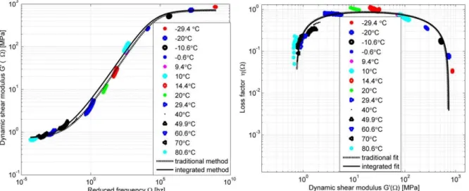
Based on the experimental data provided by Lab C (Jones, 1992), the complex Young’s and shear moduli are identi-fied by means of the traditional and the integrated methodologies. For each situation, the viscoelastic parameters ob-tained are presented in Table 3. In addition, the fitting results can be compared graphically in Figure 7 and Figure 8. Based on the identified models for both complex moduli (Table 3), the complex Poisson’s ratio is obtained using Eq. (11). As different results are found, each method is discussed in detail below.

(12)

Figure 8: Lab C. Experimental data and fitted models for the complex shear modulus: Dynamic shear modulus (left) and wick-et plot (right).

4.1.1 Traditional identification methodology

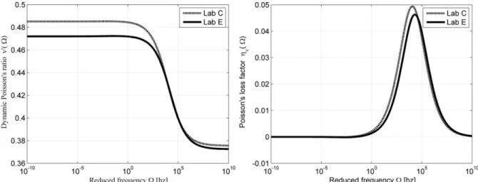
Regarding the traditional method, one observes an adequate fit for the complex Young’s modulus (Figure 7) and the complex shear modulus (Figure 8). On the other hand, by analyzing the graphics referring to the complex Poisson’s ratio (Figure 9), one observes that the dynamic Poisson’s ratio is not monotonically decreasing and the Poisson’s loss factor presents negative values. These behaviors violate a physical meaning that the VEM, under study, is energy-dissipating. In addition, the Poisson's ratio is greater than 0.5 what implies that the volume of the VEM would decrease in a axial traction test (negative dynamic bulk modulus) which is unlikely. These results do not have a physical meaning according to the theory presented by Tschoegl (1989), Pritz (1998, 2007) and Tschoegl et al. (2002).

Figure 9: Traditional method. Complex Poisson's ratio: dynamic modulus (left) and loss factor (right).

Additionally, when analyzing the shift factors obtained for the complex Young’s and shear moduli (Figure 10), one observes that the influence of temperature is similar for both complex moduli, in the common temperature range from -20o_{C to 20}o_{C. It must be emphasized that the complex Young’s modulus has experiments only within that range. Another}

(13)

Figure 10: Lab C. Shift factor as a function of temperature. The dotted lines refer to the traditional method and the continuous lines refers to the integrated method.

Thus, in order to characterize a consistent set of viscoelastic functions that meet the basic physical requirements, a more robust identification process is implemented based on optimization techniques, Eq. (28), in which some restrictions are inserted regarding the viscoelastic function of the complex Poisson’s ratio. Furthermore, the premise assumed here is that the complex Young’s and shear moduli have the same order of differentiation and that temperature influences both moduli equally.

4.1.2 Integrated identification methodology

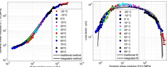
Regarding the integrated identification process, adequately fits are also observed, which are close to those obtained by using the traditional methodology (Figure 7 and Figure 8). Regarding the complex Poisson’s ratio (Figure 11), one observes that its dynamic modulus is a decreasing monotonic curve. In relation to the Poisson's loss factor, a curve is obtained with a maximum point. Furthermore, using the properties obtained from the complex Young’s and shear modu-li, one obtains the complex bulk modulus point-to-point through Eq.(9). Such function can be visualized in Figure 12. One should observe that, in this case, the complex bulk modulus is a monotonically increasing curve in the range of fre-quencies considered. In addition, such curve is located above the complex Young’s and shear moduli. Therefore, the results obtained are in accordance with the theory presented by Tschoegl (1989), Pritz (1998), and Tschoegl et al. (2002). Furthermore, Figure 10 presents a graphic representation of the shift factor in function of temperature. One observes that the shift factor obtained by the integrated method practically overlaps the curve obtained by the traditional method for the complex shear modulus. This is explained, because the experiments for the complex Young’s modulus are per-formed in a smaller temperature range (-20°C to 20°C) and, thus, the tendency is that the shift factor curve, found by the integrated methodology, follows the influence of temperature for the complex shear modulus, since it covers a broader range of temperatures.

(14)

Figure 12: Lab C. Complex viscoelastic functions (bulk, Young's and shear): dynamic modulus (left) and wicket plot (right).

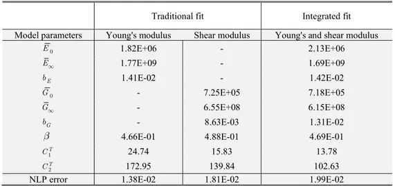
Table 3: Lab C. Identified properties of the complex viscoelastic functions (Young's and shear) by traditional and integrated methods.

Traditional fit Integrated fit

Model parameters Young's modulus Shear modulus Young's and shear modulus

0

E 1.82E+06 - 2.13E+06

E_ 1.77E+09 - 1.69E+09

E

b 1.41E-02 - 1.42E-02

0

G - 7.25E+05 7.18E+05

G - 6.55E+08 6.15E+08

G

b - 8.63E-03 1.31E-02

 4.66E-01 4.88E-01 4.69E-01

1

T

C 24.74 15.83 13.78

2

T

C 172.95 139.84 102.63

NLP error 1.38E-02 1.81E-02 1.99E-02

4.2 IDENTIFICATION OF THE VISCOELASTIC PARAMETERS – LABORATORY E

Using the experimental data produced by Lab E, similarly to the previous section, the identification of viscoelastic material EAR®

-C1002 is performed through the traditional and the integrated methodologies. The fitting results are visu-alized graphically in Figure 13 and in Figure 14. The values of the properties obtained in the optimization process are presented in Table 4.

Thus, through the identified models, one obtains the complex Poisson’s ratio (Figure 9 and Figure 11). Since differ-ent viscoelastic functions are obtained, the main characteristics of each methodology are indicated below.

4.2.1 Traditional methodology

Regarding the traditional method, one notices that the analytical models are adequately fitted to the experimental data (Figure 13 and Figure 14). However, analyzing the complex Poisson’s ratio modulus (Figure 9), one notices inade-quate behaviors for the dynamics modulus and the loss factor related to it. The first is dynamic Poisson's ratio is not monotonically decreasing, which violates a physical meaning that the VEM under analysis is a damping material. Fur-thermore, the dynamic Poisson's ratio is 0.5 which implies that the VEM is a perfectly incompressible material which is unlikely. Thus, according to Tschoegl (1989), Pritz (1998), Tschoegl et al. (2002), and Pritz (2007), such behavior has no physical significance.

(15)

between -20°C and 55°C. It must be pointed out that experimental data for the complex Young’s modulus lie only within that range.

Thus, in order to obtain physically coherent results – for the complex Poisson’s ratio – it's supposed that the tem-perature influences in the same way the mechanical behavior of the complex Young's and shear moduli, and that both moduli have the same order of differentiation (as carried out by Chen et al. 2017). In addition, constraints are inserted into the standard optimization problem, Eq. (28), preventing the inadequate physical behavior of the complex Poisson’s ratio function. Next, the characterization results obtained by the integrated method are discussed, involving experimental data of complex Young’s and shear moduli, simultaneously.

Figure 13: Lab E. Experimental data and fitted models for the complex Young's modulus: dynamic modulus (left) and wicket plot (right).

(16)

Figure 15: Lab E. Shift factor as a function of temperature. The dotted lines refer to the traditional method and the continuous lines to the integrated method.

4.2.2 Integrated methodology

Using the integrated methodology, the complex moduli (Figure 13 and Figure 14) are identified and, by relating them, one obtains the complex Poisson’s ratio (Figure 11). It should be noted that, for the proposed methodology, the function obtained for the complex Poisson's ratio is coherent, for its dynamic modulus is a decreasing monotonic curve, along frequency, and its loss factor has a maximum point. In addition, based on both complex moduli identified,

E

*

( )



and

G

*

( )



, one obtains the complex bulk modulus, using Eq. (9), in the frequency domain. Those three complex moduli may be graphically visualized in Figure 16. One observes that the complex bulk modulus is an increasing monotonic function, along frequency, and that its curve is above the other two complex moduli (Young’s and shear). These results are in accordance with the theory presented by Pritz (1998) and Tschoegl et al. (2002).

(17)

Table 4: Lab E: Properties identified for the complex dynamic and shear modulus through traditional and integrated methods

Traditional fit Integrated fit

Dynamic properties Shear properties Dynamic and shear properties

0

E _2.17E+06 - _2.10E+06

E 1.83E+09 - 2.02E+09

E

b _7.13E-03 - _1.03E-02

0

G - _7.20E+05 _7.13E+05

G - 7.12E+08 7.35E+08

G

b - _7.29E-03 _9.60E-03

 _5.43E-01 _4.84E-01 _4.73E-01

1

T

C _16.17 _19.31 _15.92

2

T

C _133.80 _157.97 _111.08

NLP error 2.03E-02 2.20E-02 2.77E-02

Additionally, Figure 15 presents a graphic of the shift factor in function of the temperature. One notices that, despite the fact the numerical results present small differences for the constants of the WLF model (Table 4), the function of the shift factor obtained by the integrated methodology (Figure 15) follows a behavior similar to those presented by the tra-ditional method. This fact makes it possible to apply the methodology in a reliable way.

5 CONCLUSIONS

The present paper discusses two methodologies for identifying mechanical properties of linear and thermorheologi-cally simple VEMs, here referred to as the ‘traditional method’ and the ‘integrated method’. Both methodologies use hybrid optimization process (GA and NLP) to obtain the optimum material parameters. As constitutive model, one em-ploys the fractional Zener model.

One observes that, by using the traditional methodology, the models are adequately fitted to the experimental data. However, the curve of the dynamic modulus and the loss factor of the complex Poisson’s ratio present inadequate behav-iors. Such results have no physical meaning and diverge from the theory. Consequently, one infers that a more robust procedure is needed in order to obtain a consistent set of viscoelastic functions, which can meet the basic physical re-quirements.

In this context, a new methodology is implemented, here referred to as ‘integrated’. Such methodology is based on the premise that temperature influences equally the mechanical behaviors of the complex Young’s and shear moduli and, in addition, such complex moduli have the same order of differentiation. Furthermore, in the optimization process, some constraints are imposed to the complex Poisson’s ratio viscoelastic function. As result, adequate fits are obtained of the analytical models to the experimental data. Besides, the dynamic modulus of the complex Poisson’s ratio proves to be monotonically decreasing and the Poisson's loss factor has a maximum point. Furthermore, based on the models identi-fied for the complex Young’s and shear moduli, one obtains the complex bulk modulus. One notices that the presented curve is monotonically increasing, along frequency, and that it is located above the complex Young’s and shear moduli. Such results are coherent with the theory, for both complex Poisson’s ratio and the complex bulk modulus have a physi-cal significance.

Therefore, considering the experiments reported here, the current paper presents a robust and efficient methodology for a hybrid characterization of the complex moduli (Young's and shear) and, subsequently, to obtain the complex Pois-son’s ratio and the complex bulk modulus for linear and thermorheologically simple solid VEMs.

Acknowledgement

(18)

References

Allou, F., Takarli, M., Petit, C., Absi, J., (2015). Numerical finite element formulation of the 3D linear viscoelastic mate-rial model: Complex Poisson's ratio of bituminous mixtures. Archives of Civil and Mechanical Engineering 15: 1138-1148.

Agirre, M. M., Elejabarrieta, M.J., (2010). Characterization and modeling of viscoelastically damped sandwich struc-tures. International Journal of Mechanical Sciences 52: 1225–1233.

Bagley, R. L., Torvik, J., (1986). On the fractional calculus model of viscoelastic behavior. Journal of Rheolology 30: 133-155.

Benedetto, H. D., Delaporte, B., Sauzéat, C., (2007). Three-Dimensional Linear Behavior of Bituminous Materials: Ex-periments and Modeling. International Journal of Geomechanics 7: 149-157.

Brinson, H.F., Brinson, L.C., (2008). Polymer Engineering Science and Viscoelasticity: An Introduction, Springer (New York).

Booij, H. C., Thoone, G. P. J. M., (1982). Generalization of Kramers-Kronig transforms and some approximations of relations between viscoelastic quantities. Rheologica Acta 21: 15-24.

Chen, D. L., Chiu, T. C. C., Yang, P. F., Jiam, S. R., (2017). Interconversions between linear viscoelastic functions with a time-dependent bulk modulus. Mathematics and Mechanics of Solids March: 1-17.

Ciniello, A. P. D., Bavastri, C. A., Pereira, J. T., (2016). Identifying mechanical properties of viscoelastic materials in time domain using the fractional Zener model. Latin American Journal of Solids and Structures 14:131-152.

Cui, H. R., Tang, G. J., Shen, Z. B., (2016). Study on the Viscoelastic Poisson's Ratio of Solid Propellants Using Digital Image Correlation Method. Propellants, Explosives, Pyrotechnics 41: 835-843.

Dandekar, D. P., Green, J. L., Hankin, M., Martin, A. G., Weisgerber, W., swanson, R. A., (1991). Deformation of ISO-DAMP (a polyvinyl chloride-based elastomer) at various loading rates. US army laboratory command materials technol-ogy laboratory may: 1-30.

Emri, I., Prodan, T., (2006). A Measuring System for Bulk and Shear Characterization of Polymers. Experimental Me-chanics 46: 429-439.

Ernst, L. J.; Zhang, G. Q.; Bressers, H. J. L., (2003). Time and temperature dependent thermo-mechanical modeling of a packaging molding compound and its effect on packaging process stresses. Journal of Electronic Packaging 125: 539-548.

Espíndola, J. J., Bavastri, C. A., Lopes, E. M. O., (2006). Design of optimum systems of viscoelastic vibration absorbers for a given material based on the fractional calculus model. Journal of Vibration and Control 14: 1607:1630.

Espíndola, J. J., Silva Neto, J. M., Lopes, E. M. O., (2005). A generalised fractional derivative approach to viscoelastic material properties measurement. Applied Mathematics and Computation 164: 493–506.

Ferry, J. D., (1980). Viscoelastic Properties of Polymers, John Wiley & Sons (New York).

Fillers, R.W., Tschoegl, N.W., (1977). The effect of pressure on the mechanical properties of polymers. Transactions of the Society of Rheology 21: 51-100.

(19)

Glöckle, W.G., Nonnenmacher, T.F., (1994). Fractional relaxation and the time-temperature superposition principle. Rheologica Acta 33: 337-343.

Graziani, A., Bocci, M., Canestrari, F., (2014). Complex Poisson’s ratio of bituminous mixtures: measurement and mod-eling. Materials and Structures 47: 1131–1148.

Guedes, R. M., (2011). A viscoelastic model for a biomedical ultra-high molecular weight polyethylene using the time– temperature superposition principle. Polymer Testing 30: 294-302.

Hecht, F. M.; Rheinlaender, J.; Schierbaum, N.; Goldmann, W.; Fabry, B; Schaffer, T., (2015). Imaging viscoelastic properties of live cells by AFM: power-law rheology on the nanoscale. Soft Matter 11: 4584-4591.

Jones, D. I. G., (1974). Temperature-frequency dependence of dynamic properties of damping materials. Journal of Sound and Vibration 33: 451-470.

Jones, D., (1992), Results of a round-robin test program: complex modulus properties of a polymeric damping material, USAF Report WL-TR-92-3104.

Kabeer, K., Attenburrow, G., Picton, P., Wilson, M., (2013). Development of an image analysis technique for measure-ment of Poisson’s ratio for viscoelastic materials: application to leather. Journal of Materials Science 48:744-749.

Koppelman, V. J., (1959). Uber den dynamischen elastizitaitsmodul yon polymethacrylsiiuremethylester bei sehr tiefen frequenzen. Colloid and Polymer Science 164:31-34.

Lakes, R. S., Winemam, A., (2006). On Poisson’s ratio in linearly viscoelastic solids. Journal of Elasticity 85: 45-63.

Kazem, S., (2013). Exact Solution of Some Linear Fractional Differential Equations by Laplace Transform. International Journal of Nonlinear Science 16: 3-11.

Kugler, H. P., Stacer, R. G., Steimle, C., (1990) Direct Measurement of Poisson's Ratio in elastomres. Amecan Chemical Society October: 17-20.

Lemini, G., (2014). Engineering Viscoelasticity, Springer (New York).

Li, C., Zeng, F., (2015). Numerical Methods for Fractional Calculus, CRC Press: New York.

Mainardi, F., (2010). Fractional Calculus and Waves in Linear Viscoelasticity – An Introduction to Mathematical Mod-els, Imperial College Press (London).

Mainardi, F., Spada G. (2011). Creep, relaxation and viscosity properties for basic fractional models in rheology. The European Physical Journal Special Topics 193:133-160.

Nashif, A. D., Jones, D. I. G., Henderson, J., P. (1985). Vibration Damping, John Wiley & Sons (New York).

Nayfeh, S. A., (2004). Damping of flexural vibration in the plane of lamination of elastic–viscoelastic sandwich beams. Journal of Sound and Vibration 276: 689-711.

O’Brien, D. J., Sottos, N. R., White, S. R., (2007). Cure-dependent Viscoelastic Poisson’s Ratio of Epoxy. Experimental Mechanics 47: 237-249.

(20)

Park, S. W., Schapery, R. A., (1999). Methods of interconversion between linear viscoelastic material functions. Part I - A numerical method based on Prony series. International Journal of Solids and Structures 36: 1653-1675.

Philippoff, W., Brodnyan, J., (1955). Preliminary results in measuring dynamic compressibilities. Journal of Applied Physics 26:846-849.

Pritz, T., (1996). Analysis of four-parameter fractional derivative model of real solid materials, Journal of Sound and Vibration 195:103-115.

Pritz, T., (1998). Frequency dependences of complex moduli and complex poisson’s ratio of real solid materials. Journal of Sound and Vibration 214:83-104.

Pritz, T., (2000). Measurement methods of complex Poisson’s ratio of viscoelastic materials. Applied Acoustics 60:279-292.

Pritz, T., (2003). Five-parameter fractional derivative model for polymeric dampingmaterials. Journal of Sound and Vi-bration 265: 935–952

Pritz, T., (2007). The Poisson’s loss factor of solid viscoelastic materials. Journal of Sound and Vibration 306:790 – 802.

Rahman, A. S. M., Tarefder, R. A., (2016). Interconversion of frequency domain complex modulus to time domain mod-ulus and compliance of asphalt concrete: numericalModeling and laboratory validation. International Mechanical Pro-ceedings of the ASME 2016 Engineering Congress and Exposition 1-10.

Renaud, F., Dion, J. L., F., Chevallier, G., Tawfiq, I., Lemaire, E., (2011). A new identification method of viscoelastic behavior: Application to the generalized Maxwell model,Mechanical Systems and Signal Processing 25: 991-1010

Ribeiro, E. A., Pereira, J. T., Bavastri C. A., (2015). Passive vibration control in rotor dynamics: optimization composed support using viscoelástico materials, Journal of Sound and Vibration 351: 43-56.

Rouleau, L., Pirk, R., Pluymers, B., Desmet, W., (2015). Characterization and modeling of the viscoelastic behavior of a self-adhesive rubber using dynamic mechanical analysis tests. Journal of Aerospace Technology and Management 7:200-208.

Sim, S., Kim, K. J., (1990). A method to determine the complex modulus and poisson’ s ratio of viscoelastic materials for fem applications. Journal of Sound and Vibration 141: 71-82.

Sousa, T. L., Kanke, F., Pereira, J. T., Bavastri, C. A., (2017). Property identification of viscoelastic solid materials in nomograms using optimization techniques. Journal of Theoretical and Applied Mechanics 55: 1285-1297.

Szabo, J. P., Keough, I. A., (2002). Method for analysis of dynamic mechanical thermal analysis data using the Havrili-ak–Negami model. Thermochimica Acta 15: 1-12

Theocaris, P. S., (1968). Interrelation between dynamic moduli and compliances in polymers. Kolloid-Zeitschrift und Zeitschrift für Polymere 1: 1182-1188.

Thomson, K. C., (1966). On the complex Poisson’s ratio of a urethane rubber compound. Journal of Applied and Poly-mer Science 10:1133-1136.

Tschoegl, N. W. (1989). The Phenomenological Theory of Linear Viscoelastic Behavior: An Introduction, Springer (New York).

(21)

Ward, I. M.; Sweeney, J. (2004). An Introduction to the Mechanical Properties of Solid Polymers, John Wiley & Sons (Chichester).

Waterman, H. A., (1977). Relations between loss angles in isotropic linear viscoelastic materials. Rheologica Acta 16: 31-42.