Rui Miguel Correia Portela

A maioria dos autores que se dedicam a estudar este tema (Feldmann & Johnson, s.d; Raymond, 1994; Hammer, 2007) identifica cinco situações principais de tomada de reféns: (a)

Segundo esse mesmo autor (idem), propostas e práticas educativas de cunho social são destinadas a pessoas e grupos em situação de risco ou necessidade de cuidado; em

Comparison of average liver size before treatment with level size one year and five years later (Table 7) showed statistically significant reduction during the

Existe grande potencial no uso de fibra de coco como substrato agrícola para o desenvolvimento de espécies vegetais cultivadas e o bom desempenho constatado nesse substrato

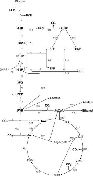
A considerable number of mechanisms were tested (results not shown). The pathway proposed in Fig. 1 b) fulfilled multiresponse regression analysis of the experimental data.

Table 1 gives the values of statistically significant Pearson’s Correlation Coefficients for the independent variables (social indicators) with two dependent variables

With these novel regulation data for a diatom polyphosphate polymerase, and their link to cellular polyphosphate changes, the transcript or protein may be used to track

Gene induction was shown for some genes up-regulated at the proteome level ( clp L/ gro EL/ rbs K), while the response of others to high hydrostatic pressure at the transcriptome