Essays on monetary policy and financial integration

Texto

(1)UNIVERSIDADE DE LISBOA Lisbon School of Economics and Management. Essays on monetary policy and financial integration Inês da Cunha Cabral Supervisor Doctor João Carlos Henriques da Costa Nicolau, Full Professor, Lisbon School of Economics and Management – Universidade de Lisboa. Thesis submitted for the degree of Doctor in Applied Mathematics for Economics and Management. 2020.

(2) UNIVERSIDADE DE LISBOA Lisbon School of Economics and Management. Essays on monetary policy and financial integration Inês da Cunha Cabral Supervisor Doctor João Carlos Henriques da Costa Nicolau, Full Professor, Lisbon School of Economics and Management – Universidade de Lisboa. Thesis submitted for the degree of Doctor in Applied Mathematics for Economics and Management Jury President Doctor Nuno João de Oliveira Valério, Full Professor and President of the Scientific Board, Lisbon School of Economics and Management – Universidade de Lisboa. Vowels Doctor João Carlos Henriques da Costa Nicolau, Full Professor, Lisbon School of Economics and Management – Universidade de Lisboa Doctor José Joaquim Dias Curto, Associate Professor with Aggregation, ISCTE Business School – Instituto Universitário de Lisboa Doctor Diana Elisabeta Aldea Mendes, Associate Professor, ISCTE Business School – Instituto Universitário de Lisboa Doctor Nuno Ricardo Martins Sobreira, Assistant Professor, Lisbon School of Economics and Management – Universidade de Lisboa Doctor Mariya Gubareva, Adjunct Professor, Lisbon Accounting and Business School (ISCAL) – Instituto Politécnico de Lisboa. 2020 ii.

(3) Abstract This doctoral dissertation consists of three separate essays on monetary policy and financial integration. The first paper explores the inflation dynamics of the Group of Seven (G7) in the period 1999.01-2018.06. Overall, there is evidence that the convergence of inflation to the reference rate of 2% tends to be slower and more disperse across countries in the case of negative variations. Additionally, the outcomes suggest that, in some cases, larger deviations are tackled at a higher speed and hint the existence of tolerance bands that are also consistent with the price stickiness theory. Finally, the empirical results stress the heterogeneity of the G7 and the euro area. The second essay analyses the relationship between changes in euro area short-term and long-term market-based inflation expectations from 2005.01 to 2018.09 and assesses the impact of oil market dynamics on these variables. The empirical findings reveal that, in each of the three subsets, the conditional correlation between changes in short-term and long-term inflation compensation is constant and relatively low. Additionally, there are no signals of fundamental deviations in how they affect each other. Also, there is evidence that changes in short-term inflation expectations respond to movements of oil prices, while changes in longerterm ones started reacting to crude dynamics in 2008. The third investigation assesses the relationship between stocks and sovereign bonds of the first wave of euro area countries from 1999.01 to 2018.09. These co-movements are analysed at different scales for three subsets. The outcomes support relevant and time-varying linkages, which also differ across countries and depend on the time scale. Moreover, the scaling properties of cross-correlations vary according to the sign of the time series trend. Finally, cross-country investigation reveals that, during turmoil periods, agents tend to invest in more robust economies and take the instrument and its jurisdictions into account.. JEL Classification: C1, C5, E5, F3, G1 Keywords: Monetary policy, Financial integration, Inflation, Inflation expectations, Capital markets iii.

(4) Resumo Esta tese é composta por três ensaios independentes que abordam temas relacionados com a política monetária e a integração financeira. O primeiro ensaio explora a dinâmica da inflação dos países que integram o Grupo dos Sete (G7) entre 1999.01 e 2018.06. Globalmente, a convergência da inflação para a taxa de referência de 2% tende a ser mais lenta e mais dispersa entre países no caso de variações negativas. Os resultados sugerem ainda que, nalguns casos, os desvios maiores são resolvidos mais rapidamente e apontam para a existência de bandas de tolerância, também consistentes com a teoria de rigidez de preços. Por fim, enfatiza-se a heterogeneidade do G7 e da área do euro. O segundo estudo analisa a relação entre as variações de nível das expectativas de inflação de curto e longo prazo da área do euro e avalia o impacto do petróleo sobre estas variáveis entre 2005.01 e 2018.09. Os resultados revelam que, nos três subperíodos, a correlação condicional entre as variações das expectativas de inflação de curto e longo prazo é constante e relativamente baixa. Adicionalmente, não há sinais de desvios fundamentais na forma como se afetam mutuamente. Verifica-se ainda que as variações das expectativas de inflação de curto prazo respondem aos movimentos do petróleo e que as de longo prazo começaram a reagir em 2008. O terceiro ensaio explora a relação entre as ações e as obrigações dos países que primeiramente integraram a área do euro no período 1999.01-2018.09. Os resultados evidenciam a existência de relações relevantes e variáveis no tempo que diferem entre países e de acordo com a escala temporal. Adicionalmente, verifica-se que as correlações cruzadas oscilam consoante o sinal da tendência da série. Por fim, constata-se que, nos períodos de crise, os agentes investem em jurisdições economicamente mais estáveis, tomando em consideração os fatores instrumento e jurisdição.. Classificação JEL: C1, C5, E5, F3, G1 Palavras-chave: Política Monetária, Integração Financeira, Inflação, Expectativas de inflação, Mercado de capitais iv.

(5) Acknowledgements I would like to express my deepest gratitude to my supervisor, Doctor João Nicolau, for his prompt cooperation and enlightening expertise. I am also thoroughly indebted to Pedro Pires Ribeiro for the continuous collaboration and encouragement to move forward in this endeavour. To my parents, brothers and grandparents my sincere thanks as this dissertation would not have been possible without their unconditional support and inspiration throughout my life. Special words of gratitude go also to my friends and professors who have followed my academic path.. v.

(6) To my family. vi.

(7) Table of Contents Abstract ..................................................................................................................................... iii Resumo ...................................................................................................................................... iv Acknowledgements .................................................................................................................... v Table of Contents ....................................................................................................................... 1 List of Tables .............................................................................................................................. 3 List of Figures ............................................................................................................................ 4 1.. Introduction ..................................................................................................................... 6. 2. Inflation in the G7 and the expected time to reach the reference rate: a nonparametric approach................................................................................................................................ 12 2.1.. Introduction ............................................................................................................ 13. 2.2.. Econometric methodology ..................................................................................... 16. 2.3.. Sample.................................................................................................................... 20. 2.4.. Empirical results .................................................................................................... 21. 2.5. 3.. 4.. 2.4.1.. Preliminary analysis .................................................................................... 21. 2.4.2.. Expected time.............................................................................................. 22. 2.4.3.. Cluster analysis ........................................................................................... 25. Conclusion ............................................................................................................. 28. Changes in inflation compensation and oil prices: short-term and long-term dynamics .. ....................................................................................................................................... 30 3.1.. Introduction ............................................................................................................ 31. 3.2.. Econometric methodology ..................................................................................... 34. 3.3.. Sample.................................................................................................................... 36. 3.4.. Empirical results .................................................................................................... 39. 3.5.. Conclusion ............................................................................................................. 46. Tracking the relationship between euro area equities and sovereign bonds ................. 49 4.1.. Introduction ............................................................................................................ 50. 4.2.. Econometric methodology ..................................................................................... 53 4.2.1.. Correlation .................................................................................................. 53. 4.2.2.. Causality ..................................................................................................... 56. 4.3.. Sample.................................................................................................................... 57. 4.4.. Empirical results .................................................................................................... 59 4.4.1.. Preliminary analysis .................................................................................... 59. 1.

(8) 4.5. 5.. 4.4.2.. DCCA: Long-range cross-correlation ......................................................... 59. 4.4.3.. ADCCA: Asymmetric long-range cross-correlation .................................. 67. 4.4.4.. Causality ..................................................................................................... 70. Conclusion ............................................................................................................. 72. Conclusion ..................................................................................................................... 75. APPENDIX .............................................................................................................................. 78 Bibliography ............................................................................................................................. 83. 2.

(9) List of Tables Table 3.1 - Descriptive statistics and preliminary tests for the original series......................... 38 Table 3.2 - Descriptive statistics for the time series in first differences .................................. 38 Table 3.3 - VAR-X-CCC-GARCH models estimates for the period from 2005.01 to 2008.06 .................................................................................................................................................. 40 Table 3.4 - VAR-X-CCC-GARCH models estimates for the period from 2008.07 to 2014.07 .................................................................................................................................................. 42 Table 3.5 - VAR-X-CCC-GARCH models estimates for the period from 2014.08 to 2018.09 .................................................................................................................................................. 44 Table 4.1 - Average of DCCA coefficients from 1999.01 to 2007.06 for different time scales intervals .................................................................................................................................... 61 Table 4.2 - Average of DCCA coefficients from 2007.07 to 2012.06 for different time scales intervals .................................................................................................................................... 64 Table 4.3 - Average of DCCA coefficients from 2012.07 to 2018.09 for different time scales intervals .................................................................................................................................... 66 Table 4.4 - Average of DCCA coefficients over the three sub-periods for different time scales intervals .................................................................................................................................... 68 Table 4.5 - Causality between equity and sovereign bonds over the three sub-periods........... 71. 3.

(10) List of Figures Figure 2.1 - Illustrating map (2.1) ............................................................................................ 17 Figure 2.2 - Evolution of inflation of the G7 from 1999 to mid-2018 ..................................... 20 Figure 2.3 - Expected time curves from 1999 to mid-2018 ..................................................... 22 Figure 2.4 - Scatter plot of average expected reversion time versus average inflation from 1999 to mid-2018 ..................................................................................................................... 24 Figure 2.5 - Panel A - Dendrogram for the average expected reversion time for G7 .............. 25 Figure 2.5 - Panel B - Dendrogram for the average expected reversion time without JP ........ 25 Figure 2.6 - Panel A - Dendrogram for the average expected reversion time: negative deviations of inflation from the 2%.......................................................................................... 26 Figure 2.6 - Panel B - Dendrogram for the average expected reversion time: negative deviations of inflation from the 2% without JP........................................................................ 26 Figure 2.7 - Panel A - Dendrogram for the average expected reversion time: positive deviations of inflation from the 2%.......................................................................................... 27 Figure 2.7 - Panel B - Dendrogram for the average expected reversion time: positive deviations of inflation from the 2% without JP........................................................................ 27 Figure 3.1 - Evolution of market-based inflation expectations and oil prices over the full sample period ........................................................................................................................... 37 Figure 4.1 - Evolution of equity and sovereign bonds over 1999-2018 ................................... 58 Figure 4.2 - Panel A - 2 nd order average fluctuation function (absolute value) for the period 1999.01 to 2007.06 ................................................................................................................... 60 Figure 4.2 - Panel B - DCCA coefficients between equity and sovereign bonds from 1999.01 to 2007.06 ................................................................................................................................. 60 Figure 4.2 - Panel C - Cross-country DCCA coefficients between equity and sovereign bonds from 1999.01 to 2007.06 .......................................................................................................... 61 Figure 4.3 - Panel A - 2 nd order average fluctuation function (absolute value) for the period 2007.07 to 2012.06 ................................................................................................................... 62 Figure 4.3 - Panel B - DCCA coefficients between equity and sovereign bonds from 2007.07 to 2012.06 ................................................................................................................................. 63 Figure 4.3 - Panel C - Cross-country DCCA coefficients between equity and sovereign bonds from 2007.07 to 2012.06 .......................................................................................................... 63. 4.

(11) Figure 4.4 - Panel A - 2 nd order average fluctuation function (absolute value) for the period 2012.07 to 2018.09 ................................................................................................................... 65 Figure 4.4 - Panel B - DCCA coefficients between equity and sovereign bonds from 2012.07 to 2018.09 ................................................................................................................................. 65 Figure 4.4 - Panel C - Cross-country DCCA coefficients between equity and sovereign bonds from 2012.07 to 2018.09 .......................................................................................................... 66. 5.

(12) 1. Introduction This dissertation comprises three separate and self-contained papers, which globally address topics in the realm of monetary policy and financial integration. At present, the primary monetary policy objective of many central banks is to achieve price stability, i.e. low and stable inflation, and even for those central banks with dual mandates, this is often seen as a necessary condition to attain other mandated objectives. Over recent decades the monetary policy frameworks of the different central banks have been subject to significant changes. In particular, since the late 1980s, inflation targeting has emerged as the most prominent structure (see, e.g. Bratsiotis et al., 2015 or Canarella and Miller, 2017) where central banks publicly announce a target inflation rate and resort to monetary policy tools to address the gap between the current rate and the reference one. Under such inflation targeting regimes, the credibility of the monetary policy thus depends on the extent to which inflation expectations across agents remain stable and close to the central banks’ reference rate, especially in the long-run. In fact, long-run inflation expectations are especially relevant in comparison to the shorter ones as they are considered the equilibrium level towards which inflation would converge after the effects of short-term shocks have vanished out and monetary policy has become fully effective. In this way, it is documented (see, e.g. Nautz et al., 2017) that well-anchored inflation expectations are not supposed to respond to macroeconomic news and should display a minimal amount of volatility. On the contrary, macroeconomic news may change short-term inflation expectations. Given the relevance of this topic, namely for policymakers, this thesis contributes to the economic literature by exploring the inflation trajectory in relation to the reference rate. This assessment is conducted for various levels and signs of deviations and for different jurisdictions whose central banks set the price stability benchmark rate at or close to 2% over the medium term. Additionally, this dissertation aims at shedding new light on the relationship between changes in short-term and long-run inflation expectations as prior research is mainly focused on how short-run inflation expectations affect longer-term ones. In this analysis a special attention is also devoted to the potential effects of oil prices on the aforementioned variables as movements in crude prices have also been associated with macroeconomic and financial changes. Without prejudice to the objective of maintaining price stability, central banks also have a keen interest in financial integration since it fosters the smooth and balanced transmission of 6.

(13) monetary policy and contributes to safeguard the financial stability of the whole financial system. Specifically, this is a prerequisite in the euro area to make the Economic and Monetary Union (EMU) sustainable as expressed in the Eurosystem’s mission statement. Indeed, financial integration in the euro area should promote risk sharing mechanisms, which are particularly relevant in a context where important adjustment structures to address asymmetries, for example related to the fiscal policy and exchange rates, are limited. Nevertheless, if it helps economies to absorb shocks and fosters development, this greater interconnection has also exacerbated the risk of cross-border financial contagion. Monitoring and understanding the main financial market segments of the euro area, which includes, among others, the bond and equity markets, is therefore crucial as stressed by central banks and academic institutions. With a greater focus on the EMU, this thesis also draws some financial integration considerations especially as regards the evolution of the capital market since the third stage of the EMU. This is a pertinent topic that deserves to be analysed, provided the relevance of integrated capital markets to offer a wider source of financing and lower funding costs for households and companies, ultimately supporting innovation and the efficient allocation of capital. In what follows, this section summarises each of the three papers by explaining the respective contribution to the monetary policy and/or financial integration, describing the methodology applied and outlining the main conclusions.. Inflation in the G7 and the expected time to reach the reference rate: a nonparametric approach Section 2 presents the first paper which falls within the scope of monetary policy. Given the importance of price stability to promote economic growth and employment, this essay aims to contribute to the literature on this topic by providing further details on the inflation dynamics in the Group of Seven (G7) from 1999.01 to 2018.06. Accordingly, for each country, it is determined the expected time that inflation takes to cross the reference level considering different levels and signs of deviations. Additionally, based on the estimates obtained, this paper sets a comparison of the inflation adjustment processes across various jurisdictions. To achieve this goal, it is entertained the Nicolau (2017)’s estimator, which consists of a procedure formulated in a completely nonparametric framework, thereby overcoming 7.

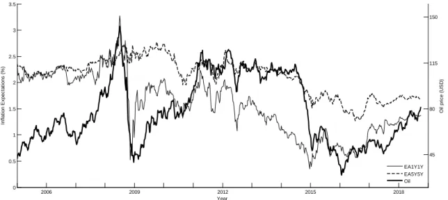
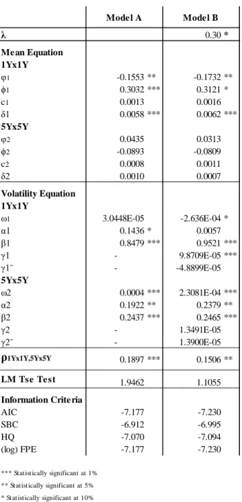
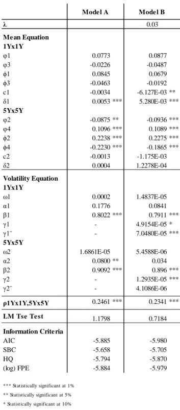
(14) specification errors, and relying on only two assumptions, i.e. stationarity and the Markovian property. The econometric literature offers few alternatives to analyse this issue. The half-life is a popular measure used to quantify the persistence of a time series, but some studies on this approach raise important questions on the precision and unbiasedness of the estimates (see, e.g. Murray and Papell, 2002). In order to compare the inflation adjustment processes of the various jurisdictions, the assessment is complemented with some cluster analyses. The estimates associated with this research convey meaningful messages on inflation dynamics. Indeed, the convergence of inflation to the reference rate tends to be asymmetric, being slower and more disperse across countries in the case of negative deviations. The empirical results also reveal that sometimes convergence to the inflation reference rate is faster when the deviation in relation to the reference rate is greater. For values of inflation fairly close to the reference rate, the outcomes advocate for the existence of tolerance bands, which can also be interpreted in light of the price stickiness literature. Furthermore, from the comparison of the inflation behaviour of the seven most powerful industrialised countries, it stands out that, notwithstanding the fact of being under a single monetary policy, idiosyncrasies of the euro area countries represented in the sample weigh on the effects of monetary policy decisions. The hierarchical clustering, which groups the G7 jurisdictions according to their features, further emphasises the heterogeneity of the group. Overall, this study is especially relevant for central banks given that the understanding of past convergence patterns and the prospects of future dynamics may support the decisionmaking process in what concerns monetary policy.. Changes in inflation compensation and oil prices: short-term and long-term dynamics The dynamics of inflation expectations may evolve differently depending on their maturity. While medium to longer-term expectations are supposed to be firmly anchored to the central bank’s objective to ensure that the monetary authority is credible, greater changes in short-term inflation expectations in response to economic and financial conditions do not necessarily point towards a weak credibility of central banks. The existent literature on the relationship between short-term and long-term inflation expectations is mainly focused on how changes in short-run inflation expectations affect longer-term inflation compensation and it is concentrated on the conditional mean structures. However, the contribution of the paper presented in Section 3 to the monetary policy domain is threefold. Firstly, it explores how the 8.

(15) interdependence of changes in euro area market-based inflation expectations with different tenors have evolved from 2005.01 to 2018.09 and, secondly, it grasps not only the mean but also the volatility features of these variables. Thirdly, taking into account that large jumps of oil prices have been followed by higher inflation, this research has an additional input to the literature by assessing the potential effects of oil prices dynamics on inflation compensation in the mean and in the variance specifications. Globally, there are two main sources of information on inflation expectations: surveys and financial markets. In particular, this study relies on inflation swaps, and especially on zerocoupon inflation swaps (ZCISR), which are the most liquid inflation derivatives that trade in the over-the-counter market. In terms of methodology, the empirical exercise draws on Vector Autoregressive (VAR) specifications for the conditional mean and on Multivariate Generalized Autoregressive Conditional Heteroskedasticity (MGARCH) models. In particular, the Constant Conditional Correlation (CCC-) model is applied given the evidence that the conditional correlations are constant rather than dynamic. Moreover, the base specification is adjusted in line with Nicolau’s (2007) approach, which was set out in the case of univariate models and resorts to a typical moving average trading rule. The rationale for this original modification is to explore the extent to which oil price movements in relation to its long-term moving average are able to influence the volatility of changes in inflation expectations. This parameterisation is then applied to three subsets that reflect distinct economic and financial conditions verified over the full sample period. As the empirical results show, this VAR-X-CCC-GARCH specification with oil effects in the volatility emerges as a preferable approach compared to other MGARCH models. From an economic perspective, the estimates bring important messages namely to the European Central Bank (ECB) who is responsible for monitoring and ensuring the anchoring of inflation expectations in order to safeguard the credibility and the effectiveness of monetary policy. At large, no fundamental deviations in how changes in short-term inflation expectations affect changes in longer-term expectations and vice versa are denoted. However, the evolution of the conditional correlation between changes in short-term and long-term inflation compensation deserves the special attention of the monetary policy authority in the near future. Similarly, the increasing sensitivity of changes in longer-term inflation compensation to crude dynamics should be further monitored.. 9.

(16) Tracking the relationship between euro area equities and sovereign bonds Financial integration is crucial for the effectiveness of a monetary union and to safeguard financial stability. Notwithstanding the introduction of the euro had marked a milestone in the history of European integration, the crises witnessed over the last years underlined some fragilities of the EMU’s architecture, triggering a series of new reforms. In particular, the launch of the Capital Markets Union, as a complement to the Banking Union, would reduce the high dependency of European businesses on banks and would constitute an important channel for risk sharing. In view of the above, it is not surprising that the Eurosystem closely monitors a wide range of indicators that allow an overall assessment of the degree of financial integration in the main euro area market segments, which includes the money market, bond markets, equity markets and banking markets, etc. The paper presented in Section 4 contributes to the academia by providing thorough information on how main euro area stocks and bonds evolved over a long time span, starting with the onset of the EMU and including the challenging economic and financial events in recent years. To this end, the data set that runs from 1999.01 to 2018.09 is divided into three subsets duly characterised by the preliminary tests. Resorting to the detrended cross-correlation analysis (DCCA), the essay evaluates comovements both within each country and across countries at different scales, which may be useful taking into account that investors in these markets usually have different investment horizons. This facet of the research is a novelty given that most of the studies that investigate euro area financial integration consider just a few lags to assess this linkage. Moreover, by employing the asymmetric version of the DCCA (ADCCA) and the Granger causality test of Toda and Yamamoto (1995), it is possible to explore eventual asymmetric features and causal relationships, respectively, which are two dimensions still underexplored in the context of the single currency. All in all, the empirical results support the pertinence of this study since there is evidence that cross-correlations and causal relationships depend on the economic and financial landscape. Moreover, the outcomes unveil that the dependence structure between stocks and bonds varies across time scales and jurisdictions, thus signalling the heterogeneity of the ten euro area countries under scrutiny. Taken together, these conclusions may contribute to improve the diversification strategies and risk mitigation techniques of agents who usually invest in several markets over different. 10.

(17) time horizons. Likewise, they may deserve the interest of policymakers as the existing studies on euro area integration are mainly focused on the stock and bond markets separately. In what follows it is developed each investigation. Therefore, Section 2 presents the first paper. Section 3 is dedicated to the second essay. Section 4 is focused on the third investigation. Finally, Section 5 concludes.. 11.

(18) 2. Inflation in the G7 and the expected time to reach the reference rate: a nonparametric approach. Abstract This paper explores the inflation dynamics of the G7 from 1999 to mid-2018 by determining the expected time so that inflation rates revert to the reference rate. Overall, this research reports four main findings. Firstly, there is evidence that the convergence of inflation to the 2% tends to be slower for negative fluctuations. Secondly, the results hint that sometimes larger deviations are tackled at a higher speed and the flat structures advocate for the existence of tolerance bands while also support the price stickiness theory. Thirdly, though sharing the same monetary policy, the euro area countries exhibit different patterns of convergence. Fourthly, the cluster hierarchy for negative variations reflects the G7 geographic location.. JEL classification: C14, C38, E52 Keywords: Monetary policy, Inflation, Asymmetry, Expected time, Markov chain 12.

(19) 2.1.. Introduction. Currently, the primary monetary policy objective of many central banks is to attain price stability and, even for those central banks with dual mandates, this is often seen as a prerequisite to achieve other mandated objectives. Admittedly, by ensuring that there is no protracted and substantial inflation or deflation, central banks contribute significantly to balanced economic growth and employment (see, e.g. Mallick and Mohsin, 2016). In order to make the monetary policy more transparent and to provide guidance to the agents as far as expectations of future price developments are concerned, many central banks have established a quantitative goal of price stability by setting an explicit inflation objective. Under such an inflation targeting regime, central banks publicly announce a target inflation rate and resort to monetary policy tools to address the gap between the current rate and the reference one. The effectiveness of such inflation targets is well documented in the literature with some researchers postulating that it is useful in reducing inflation and inflation variability (see, e.g. Vega and Winkelried, 2005 or Creel and Hubert, 2010). Gürkaynak et al. (2010) and Ehrmann (2015) also argue that an official target helps to anchor expectations on the distribution of long-run inflation outcomes. Furthermore, there are some indirect benefits of an explicit and credible reference rate in terms of controlling exchange rates (see, e.g. Lin, 2010) and the volatility of interest rates (see, e.g. Ardakani et al., 2018) and as regards the fiscal discipline (see, e.g. Minea and Tapsoba, 2014). Given that the extent to which inflation expectations are anchored on a specified target reflects the credibility of the monetary policy, it is not surprising that inflation has become one of the most analysed economic data. Against this backdrop, this paper aims to contribute to the literature on the inflation trajectory by determining the expected time that inflation takes to cross the inflation reference level in the Group of Seven (G7), i.e. Canada (CA), Germany (DE), France (FR), Italy (IT), Japan (JP), the United Kingdom (UK) and the United States (US), whose central banks set the price stability benchmark rate at or close to 2% over the medium term. This study is especially relevant in a context where there is great interest and a lively discussion on both the degree of persistence of inflation and the symmetry of its adjustment towards the long-run equilibrium. As regards inflation persistence, i.e. the extent to which the effect of a shock persists in terms of size and length, empirical issues either focus on a single jurisdiction (e.g. Meenagha et al., 2009 and Jain, 2019) or set comparisons across countries (see, e.g. Kouretas and Wohar, 13.

(20) 2012 or Ahmad and Staveley-O’Carroll, 2017). In the G7, it is worth signalling the works of Kumar and Okimoto (2007) that find a global and significant decline of inflation persistence over the period 1960-2003. Similar conclusions are drawn namely by Bataa et al. (2013) and Jung (2019) who monitor inflation rates from 1973 to 2007 and from 1960 to 2016, respectively. A tangential branch of this investigation also puts forward the factors behind this inflation persistence. Some authors claim that inflation inertia is a function of the monetary policy aggressiveness (see, e.g. Benati and Surico, 2007 or Carlstrom et al., 2009) while others advocate that inflation persistence is a consequence of aggregating prices from heterogeneous firms in their price adjustment costs (see, e.g. Mankiw and Reis, 2002 or Carvalho, 2006). Regarding the price stickiness research, it is also important to highlight the works of Ball and Mankiw (1994) and Peltzman (2000) supporting asymmetric price. Another strand of the literature elaborates on the inflation dynamics and investigates whether the speed of inflation adjustment towards its equilibrium is constant or, on the contrary, depends on how far it is above or below its long-run level or the magnitude of the positive or negative shocks hitting the inflation. This asymmetric behaviour of inflation is especially depicted in the empirical studies of Tsong and Lee (2011) and Manzan and Zerom (2015). According to Akdoğan (2015), the different pattern of convergence is determined by the asymmetric response of policymakers against upwards or downwards deviations of inflation from the target and by the dissimilar persistence of shocks to the inflation process. As for the first argument, Orphanides and Wieland (2000) argue that, despite having an inflation goal formally defined, in practice, central banks expect to keep inflation within a range rather than focusing on that rate. As the authors explain, when inflation is close to the policymakers’ bliss level, they may want to avoid deliberately changing aggregate demand that would be needed for further improvements in inflation. This different response, according to which monetary authorities react in a passive manner when inflation is within the target band and become aggressive when it deviates from it, is also addressed by Naraidoo and Raputsoane (2011). Moreover, these authors show that, when inflation is outside that zone, monetary authorities react with the same level of aggressiveness regardless of whether inflation overshoots or undershoots the inflation target band. Nevertheless, this symmetry detected is not consensual as it is acknowledged that central banks may be more biased against downward jumps in inflation rather than upwards movements or vice versa (see, e.g. Bec et al., 2002; Ruge-Murcia, 2003 or Chesang and Naraidoo, 2016). The second rationale according to which positive and negative shocks have different effects on inflation, thereby contributing to the asymmetric adjustment process of the inflation rates, is supported by 14.

(21) Tsong and Lee (2011). Erceg and Levin (2003) justify this different persistence based on the imperfect monetary policy credibility perceived by market participants. By drawing a comparison across the various jurisdictions under analysis, this paper also relates to the research on the inflation globalisation. Focusing on data regarding the Organisation for Economic Cooperation and Development (OECD) countries, Ciccarelli and Mojon (2010) detect relevant co-movements that may be due to the existence of global business cycles and to the spread of monetary policy concepts among central banks. The potential benefits of central banks’ coordination is also indirectly supported by Altansukh et al. (2017) who concur that the apparent globalisation of inflation rates may be a consequence of the adoption of similar monetary policies across jurisdictions rather than the increased transmission of foreign inflation to individual jurisdictions. In this analysis, to model G7 inflation dynamics, it is entertained the Nicolau (2017)’s estimator, which consists of a procedure formulated in a completely nonparametric framework, thus overcoming specification errors, and relying on only two assumptions, which are stationarity and the Markovian property. Prior literature recognises merits in using Dynamic Stochastic General Equilibrium (DSGE) models to assess the amplitude and persistence of the responses of inflation to various shocks (see, e.g. Christiano et al., 2010; Guerron-Quintana et al., 2017 or Phaneuf et al., 2018). In turn, to test for asymmetry in inflation persistence, Aslanidis et al. (2018) resort to the threshold autoregressive (TAR) model. Likewise, the Smooth Transition Autoregressive (STAR), such as the Exponential Smooth Transition Autoregressive (ESTAR) process (see, e.g. Gregoriou and Kontonikas, 2009 or Strohsal and Winkelmann, 2015) and its asymmetric (AESTAR) variant (see, e.g. Akdoğan, 2015) is employed to capture the nonlinear behaviour and the eventual asymmetric features of inflation data. Nevertheless, although these nonlinear models provide information on the speed of adjustment, they do not allow the quantification of the expected time so that the inflation reference rate is restored. This study then delivers these estimates for various levels and signs of deviations. The half-life, which is usually described as the number of periods required for the impulse response to a unit shock to dissipate by half, is a popular measure used to quantify the persistence of a time series. However, some studies on this approach raise some questions, especially related to the precision and unbiasedness of the estimates (see, e.g. Murray and Papell, 2002). Taking into account that this paper also envisages a comparison of the inflation adjustment processes of various jurisdictions, the assessment is complemented with some cluster analyses. On the back of this procedure, time series are divided into groups based on their features and 15.

(22) on their relationships so that data belonging to the same cluster exhibits a similar pattern. Dendrograms represent one of the cluster visualisation options. Regarding the sample, it comprises inflation data extracted on a monthly basis from Refinitiv for the G7 from 1999.01, which signals the beginning of the Economic and Monetary Union (EMU), to mid-2018. The current research conveys meaningful messages to policymakers and enriches the existent literature on inflation dynamics in different ways. Firstly, this paper not only tests for a possible asymmetry in inflation dynamics, but also assesses the time horizons so that inflation recovers from positive and negative shocks and from distinct levels of deviations from the reference rate. Secondly, instead of focusing on a single jurisdiction, this analysis sets a comparison across the seven most powerful industrialised countries and explores possible cluster structures among them. The remainder of the paper is organised as follows. Section 2.2 presents the methodology. Section 2.3 describes the data. Section 2.4 outlines and discusses the empirical results. Lastly, a brief conclusion is given in Section 2.5.. 2.2.. Econometric methodology. This section sketches the econometric modelling that is followed to provide further light on the inflation trajectories of different jurisdictions. In this way, the analysis focuses primarily on the nonparametric method proposed by Nicolau (2017) to determine the expected time to cross a certain threshold. It is worth noting that this approach is easily implemented and it is based on only two assumptions, i.e. the Markovian property and stationarity. This new estimator is now described. Supposing y is a discrete-time process with state space R and assuming that, as aforementioned, y is a Markov process of order r and y is a strictly stationary process. Under this last assumption, it can be demonstrated that the process, starting at level a that does not belong to the generic set A , almost surely visits A an infinite number of times as t → ∞.. Considering the hitting time T := Tx = min{t > 0 : yt ≥ x1 } and presume that the process starts at 1. values x0 < x1 . The case x0 > x1 with Tx = min{t > 0 : yt ≤ x1} is similar. For general non-linear 1. processes, the distribution of T is usually difficult to obtain. Nevertheless, there is a 16.

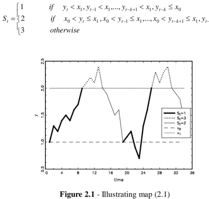
(23) nonparametric approach that allows such estimation. Let S 0 = 1 if y0 = x0 , i.e. the process starts at y0 = x0 , and then define the following transformation for 1  S t = 2 3 . k ≥0:. if. yt < x1 , yt −1 < x1 ,..., yt −k +1 < x1 , yt −k ≤ x0. if. x0 < yt ≤ x1 , x0 < yt −1 ≤ x1 ,..., x0 < yt −k +1 ≤ x1 , yt −k ≥ x1. (2.1). otherwise. Figure 2.1 - Illustrating map (2.1). Figure 2.1 exemplifies the mapping of (2.1) for a hypothetical dynamic of y . The probabilities of T can be difficult or even impossible to extract from y , but they may be easily obtained from process S t . In general, it can be demonstrated that: t −1. ∏p. P(T = t ) = (1 − pt ). i. = (1 − pt ) pt −1 pt −2 ... p1. i =1. where pt = P( St = 1 | St −1 = 1, St − 2 = 1,..., S0 = 1) . The strategy is to deal with S t as a Markov chain with state space {1,2,3} and then estimate the relevant parameters. This method is supported by the following propositions: Proposition 1: Supposing that y is a r th order Markov process. Then S is a r th order Markov chain. From the assumption that y is a Markov process of order r and from this proposition, then pt = P( St = 1 | St −1 = 1, St − 2 = 1,..., St − r = 1) . The probabilities pt can be inferred from standard Markon chain inference theory.. 17.

(24) To highlight the dependence of St on x0 and x1 the transition probability matrix is written as P( x0 , x1 ) = [Pij ( x0 , x1 )]3×3 where Pij = Pij ( x0 , x1 ) := P( St = j | St −1 = i ) . If S is a first order Markov chain, i.e. r = 1 , then pt = P( St = 1 | St −1 = 1) = P11 and E (T ) =. ∞. ∑. tpt = (1 − P11 ). t =1. ∞. ∑ tP t =1. t −1 11. =. 1 1 − P11. (2.2) ^. E (T ). can be easily estimated from the maximum likelihood estimate P11 = n11 / n1 , where n11 is. the number of transitions of type S t −1 = 1, S t = 1 and n1 is the number of ones in the sample (i.e. S t = 1 ). ^. p Proposition 2: P11 = n11 / n1 → P11 and. ^. d N (0, P11 (1 − P11 ) / π 1 ) , n ( P11 − P11 )  →. where π 1 is such that. p π1 . n1 / n →. ^. ^. Proposition 3: Let E (T ) = 1/(1 − P11 ) . In case of r = 1 : ^. p E (T )  → E (T ) ,.   P11  ^  d  , 0 < P11 < 1 n  E (T )− E (T )  → N  0, 3     (1 − P11 ) π 1  t −1. Proposition 4: Focusing now on the case of r > 1 and recalling that P(T = t ) = (1 − pt )∏ pi i =1. where pt = P( S t = 1 | S t −1 = 1, S t −2 = 1,..., S 0 = 1) . Given that pt = pr if t > r , in light of the Markovian property: t −1  − p t≤r ( 1 ) t ∏ pi ,  i =1  P(T = t ) =  r −1  t −r  (1 − p ) r ∏ pi    pr , t > r  i =1  . and therefore: t −1 r −1 r  ∞  E (T ) = ∑ t (1 − p t )∏ p i + (1 − p r )∏ p i  ∑ tp rt − r t =1 i =1 i =1 t = r +1  r −1 t −1 r ( 1 p + r − rp r )   = ∑ t (1 − p t )∏ p i + (1 − p r )∏ p i  r 2 t =1 i =1 i =1  (1 − p r ) . (2.3). that is reduced to the following formulas: r = 1 ⇒ E (T ) =. r = 2 ⇒ E (T ) =. 1 1 = 1 − p1 1 − P11. 1 + p1 − p 2 , etc. 1 − p2. 18.

(25) Since that. the. Markov. chain. is. homogeneous,. p k = P ( S k = 1 | S k −1 = 1,..., S 0 = 1) = P ( S t = 1 | S t −1 = 1,..., S t −k = 1) , k < r. p1 := P ( S1 = 1 | S 0 = 1) = P11 . The estimation of. and,. it. follows. in. particular,. pk is based on the maximum likelihood. ^. estimate pk = A / B , where A is the number of transitions from St −1 = 1,..., St − k = 1 to S t = 1 and B is the number of cases where S t −1 = 1,..., S t −k = 1 . Nevertheless, when k is relatively large and. the sample size is small the modelling of these probabilities may be problematic. Hence, k should not be higher than 4 or 5 although it depends on the sample size, the persistence level of y and the thresholds x0 and x1 . In this exercise, the threshold is equal to the reference rate of 2% of the G7 central banks and the model order is determined by analysing the partial autocorrelation function. The econometric research offers few alternatives to this approach. The half-life is a very popular measure used to quantify the persistence of a time series. However, the literature raises some questions regarding this approach, especially related to the precision and unbiasedness of the estimates (see, e.g. Murray and Papell, 2002). Additionally, half-life implies that positive and negative shocks with equal magnitude have the same effect on the impulse response function, which may not reflect the real behaviour of time series (see, e.g. Damásio et al., 2018). In order to compare the G7 in terms of expected time curves (ETC) a hierarchical clustering is also employed. During the first stage of the method, each item is considered as an individual cluster and the various objects are stepwise linked so that they are all connected at the top of the clustering. The objects are thus joined together from the closest, i.e. the most similar, to the furthest apart, i.e. the most different. The resulting tree, which can be visualised by means of a dendrogram, is built with a linkage function that measures the between-clusters dissimilarities in terms of expected time. In this process, the conventional metric of Euclidean distance is used, which is defined in general terms as:. d ( p, q ) =. k. ∑ (q i =1. − pi ). 2. i. (2.4). where p and q are two vectors and k represents the number of statistical characteristics observed.. 19.

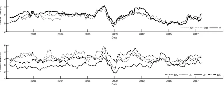
(26) 2.3.. Sample. The empirical analysis draws on monthly observations of inflation extracted from Refinitiv for the G7, i.e. for CA, DE, FR, IT, JP, UK and US. The time span of this study is large and covers the period from 1999.01 to 2018.06, which allows the meaningful estimation of the model. It is worthwhile to note that central banks of the G7 pursue the same reference level of or around 2% for inflation over the medium term. Although some of these countries only officially adhered to it after 1999, 1 they had already followed this benchmark rate in an implicit fashion. An exception to this is JP whose reference until 2012 was an inflation rate between 0% and 2%, with a focus on the midpoint of around 1%. In 2013, the Bank of Japan moved to an inflation targeting regime of 2%.. Inflation rate (%). 6 4 2 0 DE -2 1998. 2001. 2004. 2006. 2009 Date. 2012. 2015. 2001. 2004. 2006. 2009 Date. 2012. 2015. FR. IT 2020. 2017. Inflation rate (%). 6 4 2 0 -2 CA -4 1998. US. JP. UK 2020. 2017. Figure 2.2 - Evolution of inflation of the G7 from 1999 to mid-2018. The evolution of this variable for the different countries is depicted in Figure 2.2. From this graph, it can be observed that after a sharp rise in 2007 and in the first half of 2008, G7 inflation rates went on a marked downward trend as the effects of the subprime crisis became visible, in the fall of 2008. After that period, price changes even turned negative in certain cases, prompting an intense and comprehensive debate on whether disinflationary or even deflationary risks were likely to materialise and what measures would be required to avoid. 1. CA and UK were the first sample countries to implement an inflation targeting regime in the early 1990s. Although it was defined in 1998, it was only in 2003 that the ECB announced the price stability objective of an inflation rate close, but below, to 2% over the medium term. Similarly, the US Federal Reserve made the 2% goal explicit in 2012.. 20.

(27) them. Despite remaining subdued and below the reference rate, inflation rates have been trending up since 2015, in tandem with the global economic expansion.. 2.4.. Empirical results. 2.4.1. Preliminary analysis The analysis of inflation series starts with the conventional tests for the presence of unit roots. According to the results of the ADF (Dickey and Fuller, 1981) test and the PP (Phillips and Perron, 1988) test,2 inflation time series under investigation are stationary. Hence, this outcome supports the use of inflation data in levels. It is important to note that whether inflation series are best treated as stationary or nonstationary has not yet achieved consensus in the literature. Nevertheless, the stationarity identified is in line with Clemente et al. (2017) who offer evidence that inflation rates of the G7 are better characterised as integrated of order zero rather than as first order integrated variables. Also Gregoriou and Kontonikas (2006), using a nonlinear root test, argue that, although deviations of inflation from the target can exhibit a region of non-stationary behaviour, overall they are stationary, thereby signalling successful targeting implementation. Indeed, the presence of unit roots in inflation data would imply that inflation rates could reach any arbitrary value, which is precisely what central banks seek to avoid when there is a reference rate in place.. 2. Results are available upon request.. 21.

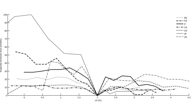
(28) 2.4.2. Expected time. 100 DE FR IT CA US JP UK. 90. Expected reversion time (months). 80. 70. 60. 50. 40. 30. 20. 10. 0. 0. 0.5. 1. 1.5. 2 x0 (%). 2.5. 3. 3.5. 4. 4.5. Figure 2.3 - Expected time curves from 1999 to mid-2018. Figure 2.3 displays the ETC for the various jurisdictions from 1999.01 to 2018.06. These estimates consider the same threshold x1 , which is assumed to be 2%, but different starting points x0 equally spaced in the intervals ]min( y, x1 ), x1 [ and ]x1 , max( y, x1 )[ . To illustrate, assume that IT’s inflation rate is currently at x 0 = 1.5% . According to Figure 2.3, the expected time for IT’s inflation path to cross the x1 = 2% threshold is about 28 months. It is interesting to note that the convergence to the reference rate tends to be slower in the case of negative deviations from the target in comparison with positive ones. This is obvious in JP that has been stuck at low inflation rates, well below the Bank of Japan’s target. Moreover, it is notorious that the dispersion of the mean expected reversion time among countries is also higher when the process approaches the reference rate from lower values. As a matter of fact, the expected time ranges between 1 and 26 months for positive deviations which compares with the interval of 2 to 100 months associated with negative variations in relation to the target. These findings can be broadly interpreted in light of the monetary policy transmission mechanism, i.e. the process through which central banks’ monetary policy decisions, conventionally taken in regards to official interest rates, ultimately affect inflation rates. Usually, in the context of economic growth and inflation above the reference rate, an increase of monetary policy interest rates tends to discourage investment and consumer spending. In the same vein, an accommodative monetary policy, which is attained by lowering policy rates 22.

(29) below the natural (or equilibrium) interest rate,3 is followed to stimulate the economy and raise inflation rates. Although historical data has proved that inflation increases to values above the target were quickly tackled in the past through higher interest rates, the same evidence is not so clear in what concerns the recent period of low inflation. Indeed, the successive decreases of monetary policy interest rates for values close to zero was not sufficient to deal with low inflation dynamics faced during the recent period. The reason for the difficulty found lies in the existence of an effective lower bound. 4 With the purpose of overcoming this issue, some central banks adopted unconventional monetary policy measures in the form of forward guidance (i.e. indications of the future course of monetary policy) and quantitative easing (i.e. large-scale asset purchases). Notwithstanding the aforementioned explanation, the quicker convergence of inflation for values higher than the reference rate is also in line with those authors who argue that the central banks’ monetary policy response is stronger and more immediate against positive deviations from the target in comparison to negative fluctuations, provided that the deviation from the inflation target is above a certain threshold (see, e.g. Martin and Milas, 2004 or Surico, 2007). From the scrutiny of Figure 2.3 it is also possible to realise that, globally, the ETC is not monotonic in both cases of downward and upward movements in relation to the reference rate, i.e. it is not entirely non-increasing and non-decreasing, respectively. De facto, in some cases, convergence is faster when the deviation is greater, which suggests that monetary policy authorities are more determined to act against larger deviations or their measures are more effective in such scenarios. This is especially visible in the intervals [0.5, 0.7], [-0.45, -0.05] and [2.9, 3.8] for UK, US and IT, respectively. Besides, it stands out that the ETC tend to be almost flat for some sequences of x0 . This is particularly clear in CA, US and IT when fluctuations are negative as well as for CA, JP and UK in case of positive deviations from the 2%. If inflation is much higher (lower) than the desirable long-run reference rate, there is not much controversy that monetary policy ought to reduce (increase) the inflation levels. However, when inflation is fairly close to the reference rate, policymakers may opt for having a moderate response or may even refrain from intervening. The so-called tolerance bands indicate comfort zones as there may be small. 3. The natural or equilibrium interest rate tends to be interpreted as the real interest rate that would prevail under conditions considered desirable from the standpoint of macroeconomic stabilisation. 4 The nominal interest rates are subject to a minimum value designated the effective lower bound. Given that cash offers zero nominal return, it would be expected that agents prefer it to any other asset offering negative nominal return rates. Yet, in practice, holding cash may incur some costs that imply that the effective lower bound of nominal interest rates may fall slightly below zero.. 23.

(30) transitory shocks responsible for inflation short-term volatility that are deemed acceptable and do not require a monetary policy response. Likewise, these ranges reflect central banks’ concern in terms of macroeconomic stabilisation that leads them to avoid excessive output and employment changes when addressing threats to price stability. Nevertheless, this almost linear behaviour can also be interpreted in the light of the price stickiness literature. As Ball and Mankiw (1995) argue, changing prices is costly and therefore firms may choose not to react if shocks are relatively small. Figure 2.3 also points out that inflation dynamics in DE, IT and FR are different since the mean expected reversion time to the reference rate diverges across these countries. For the various starting points x0 considered, FR presents more dispersed expected time values, varying from 3 to 54 months, while the bounds of DE and IT are approximately 6 to 23 months and 5 to 34 months, respectively. Although these three jurisdictions are under the single monetary policy of the Eurosystem, in practice, the effects of monetary policy decisions are not equal, which reflects the idiosyncrasies of each economy.. 4 CA DE FR. 3.5. IT JP UK US. Average inflation (%). 3. 2.5. 2. 1.5. 1. 0.5. 0 0. 10. 20. 30. 40 50 Average expected reversion time (months). 60. 70. 80. Figure 2.4 - Scatter plot of average expected reversion time versus average inflation from 1999 to mid-2018. Figure 2.4 exhibits the scatter plot of the average inflation rates against the average expected reversion time for positive and negative deviations from the reference threshold. The four quadrants are defined by the medians that take into account the entire sample. This graph denotes the higher similarity of the G7 in case of positive departures from the reference rate in terms of both, mean expected reversion time and average inflation. Looking at the results in greater detail, when assessing positive deviations of inflation from the reference rate, UK and 24.

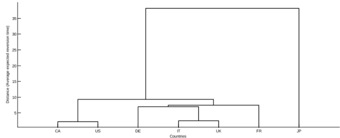
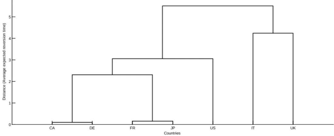
(31) IT are reported in the same quadrant, diverging from the remaining countries due to their higher average expected reversion time which lasts up to 21 and 16 months, respectively. In relation to negative fluctuations, CA and US belong to the quadrant associated with the lowest expected reversion horizons, reporting average values of 10 and 8 months, respectively.. 2.4.3. Cluster analysis. Distance (Average expected reversion time). 16. 14. 12. 10. 8. 6. 4. 2. 0. IT. FR Countries. DE. US. CA. UK. JP. Figure 2.5 - Panel A - Dendrogram for the average expected reversion time for G7. 7. Distance (Average expected reversion time). 6. 5. 4. 3. 2. 1. CA. US. DE. FR. IT. UK. Countries. Figure 2.5 - Panel B - Dendrogram for the average expected reversion time without JP. The dendrogram displayed in Panel A of Figure 2.5 reinforces the abovementioned idea that, in general, the G7 is not homogenous. Albeit this conclusion, and in line with the previous Figure, there are two pairs of jurisdictions that are fairly close in what concerns the average expected convergence time of inflation to the reference rate, which are UK and IT and CA and US. JP clearly stands apart from the remaining G7 economies and if it is excluded from this analysis, the cluster structure does not change as shown in Panel B. 25.

(32) Distance (Average expected reversion time). 35. 30. 25. 20. 15. 10. 5. CA. US. DE. UK. IT Countries. FR. JP. Figure 2.6 - Panel A - Dendrogram for the average expected reversion time: negative deviations of inflation from the 2%. 9. Distance (Average expected reversion time). 8. 7. 6. 5. 4. 3. 2 CA. US. DE. IT. UK. FR. Countries. Figure 2.6 - Panel B - Dendrogram for the average expected reversion time: negative deviations of inflation from the 2% without JP. The same analysis in terms of average expected convergence time is conducted to distinguish positive from negative deviations from the reference rate. According to Panel A of Figure 2.6, which displays the hierarchy of clusters associated with negative variations, CA and US form a well-defined cluster, thus supporting the higher similarities previously signalled in Figure 2.4. Moreover, there is evidence that the behaviour of DE, IT, UK and FR is more identical in comparison with the remaining countries. Lastly, JP stands out as having a completely different dynamic. These clusters point out the relevance of the geographic location of these countries in what respects inflation dynamics as they are grouped by continents. This pattern is also recognised by other authors when analysing different variables. For instance, when assessing the synchronisation of business cycles, Enea et al. (2015). 26.

(33) documents the existence of a euro area cycle, centred on DE, FR and IT, while highlighting JP’s unique position and behaviour within the G7. Panel B shows the results of this exercise without considering JP, providing evidence that the cluster structure remains the same.. Distance (Average expected reversion time). 5. 4. 3. 2. 1. 0. CA. FR. DE. JP Countries. US. IT. UK. Figure 2.7 - Panel A - Dendrogram for the average expected reversion time: positive deviations of inflation from the 2%. Distance (Average expected reversion time). 5. 4. 3. 2. 1. 0. CA. DE. FR. US. IT. UK. Countries. Figure 2.7 - Panel B - Dendrogram for the average expected reversion time: positive deviations of inflation from the 2% without JP. As exposed in Figure 2.7 - Panel A, this scrutiny was also conducted in relation to positive deviations and the conclusions diverge from the ones shown in Figure 2.6 - Panel A. Indeed, the location of these jurisdictions seems to be irrelevant in this context as economies from different continents unveil the greatest similarities. The shortest divergences in terms of average expected convergence time are found for the two pairs CA and DE and FR and JP. Moreover, overall, the distances associated to the various clusters are also smaller in this 27.

(34) scenario. When JP is excluded from this analysis, the cluster structure changes, as demonstrated in Panel B of Figure 2.7. However, given the dissimilarities in the inflation behaviour previously flagged (e.g. Figure 2.4), the different group features pointed out in Figures 2.6 and 2.7 are not considered unexpected.. 2.5.. Conclusion. Inflation dynamics lies at the centre of monetary policy and, as such, has motivated several empirical research. Notwithstanding the broad literature on this topic, to the best of our knowledge, the expected time it takes inflation rates to cross the reference rate has not yet been overly explored in the literature. In particular, this study aims at this quantification, distinguishing positive from negative deviations of G7 inflation rates from the 2% reference rate. The approach taken herein relies on Nicolau (2017)’s nonparametric method, which is a procedure formulated in a completely nonparametric framework by relying on only two assumptions (stationarity and the Markovian property). The clustering procedure is also entertained to complement and systematise the comparison of the various economies in what respects the ETC. At large, this paper reports some relevant conclusions. Firstly, there is evidence that downward movements of inflation from the reference rate tend to be tackled at a lower speed. Indeed, the interval of 2 to 100 months obtained in this context compares with the smaller range of 1 to 26 months identified for upward fluctuations. In line with this outcome, the various countries also exhibit higher dispersion of expected time values when the process approaches the reference rate from lower values. These conclusions may be interpreted in light of the monetary policy transmission mechanism and, more precisely, given the existence of an effective lower bound for lowering policy interest rates. Secondly, it is possible to conclude that, in certain cases, convergence is faster when the departure from the reference rate is greater, signalling that monetary authorities’ actions are more effective in such scenarios or policymakers are more determined to act against larger deviations. Furthermore, the flat structure of the ETC for smaller values of deviations advocate for the existence of tolerance bands within which inflation can fluctuate. This almost linear behaviour also supports the literature on price stickiness. Thirdly, euro area countries’ idiosyncrasies seem to weigh on the real effects of Eurosystem monetary policy decisions. In this sample, DE, FR and IT exhibit different patterns of convergence, despite being under a single monetary policy. 28.

(35) Finally, it is interesting to note that the seven countries are differently grouped depending on the sign of the deviation. In particular, the clusters obtained in the case of negative fluctuations denote G7 geographic location. Overall, this study contributes to the current literature by providing further details on the inflation process. The empirical results are especially relevant for central banks that seek to promote price stability. Definitely, the understanding of past convergence patterns and the anticipation of future dynamics have important implications on how monetary authorities should conduct monetary policy. The main takeaways of this paper raise some questions that should be addressed in future research. On the one hand, it would be interesting to explore the determinants of this asymmetric behaviour of inflation around the 2% reference rate. On the other hand, in the light of the outcomes on the EMU countries represented in this sample, similar analysis could be conducted in relation to the remaining euro area jurisdictions in order to monitor financial integration.. 29.

(36) 3. Changes in inflation compensation and oil prices: short-term and long-term dynamics. Abstract This paper investigates the relationship between changes in euro area short-term and longterm market-based inflation expectations from 2005.01 to 2018.09, also devoting special attention to the relevance of the oil market. The full sample is split into three subsets related to different economic and financial landscapes. To model the conditional mean and the variance-covariance structure, a VAR-X-CCC-GARCH specification with oil effects in the volatility proves to be a preferable approach compared to other Multivariate GARCH models. In general, the conditional correlation between changes in short-term and long-term inflation compensation appears as constant and relatively low in each subset, though increasing since mid-2014. Furthermore, there are no signals of fundamental deviations in how changes in short-term inflation expectations affect changes in longer-term expectations and vice versa. There is evidence that changes in short-term inflation expectations tend to respond to the movements of oil prices over time, while changes in longer-term ones started responding to crude dynamics after mid-2008. On the whole, these findings are relevant for analysts, investors and especially for the policymakers who are responsible for ensuring price stability.. JEL classification: E52, Q43, C51 Keywords: Monetary policy, Inflation expectations, Oil, Trading rule, Anchoring 30.

(37) 3.1.. Introduction. Inflation expectations play a crucial role in macroeconomics and especially in the sphere of monetary policy. Therefore, policymakers closely monitor the evolution of inflation expectations as one of the most relevant inputs for assessing the inflation outlook and the related risks (see, e.g. Adeney et al., 2017). By and large, it is possible to gain insight into future inflation by means of econometric forecasting models, surveys and information retrieved from financial markets. In particular, over recent years, market-implied measures of inflation expectations have become very popular as they may be readily collected for a large set of maturities and reflect the beliefs of agents who are willing to risk money based on their expectations (see, e.g. Ribeiro and Curto, 2018). Accordingly, the simplest and most frequent inflation expectation analyses draw on spot and forward rates from inflation swap rates and breakeven inflation rates. Given that inflation-linked securities are being more actively traded in financial markets and are keenly followed by analysts, market participants and policymakers, research around these instruments has also sprouted in different dimensions. One of the fields of the literature is dedicated to breaking down inflation-linked swaps (ILS) and breakeven inflation rates into ‘true’ inflation expectations and risk premia (see, e.g. Christensen et al., 2010; Haubrich et al., 2012 or Hördahl and Tristani, 2014). Indeed, without any adjustment, the straightforward reading of these measures reflects the inflation compensation demanded by economic agents for taking on inflation risk, which encompasses ‘genuine’ inflation expectations as well as inflation and liquidity risk premia (among others). In turn, some other authors have been studying the anchoring of long-term inflation expectations to the central banks’ objective (see, e.g. Beechey et al., 2011; Nautz et al., 2017 or Fracasso and Probo, 2017). Notwithstanding the relevance of anchored inflation expectations to conduct monetary policy, the knowledge about their determinants is scant. The works of Ehrmann (2015), Bauer (2015) and Glas and Hartmann (2015) aim to explore this topic by devoting particular attention to the realised inflation, the state of the economy and monetary policy measures. Finally, other authors endeavour to assess the linkage of inflation expectations across different jurisdictions (see, e.g. Bayoumi and Swiston, 2010 or Netšunajev and Winkelmann, 2014). This paper contributes to the literature by investigating the interdependence of euro area inflation expectations of different tenors throughout various time spans that encompass dissimilar economic and financial conditions. In addition, it brings further insight into the. 31.

(38) transmission mechanism, if existent, between crude and euro area inflation expectations for various time horizons. The dynamics of inflation expectations may evolve differently depending on the maturity under inspection. If the objective function of the monetary authority is credible, then medium to longer-term expectations are supposed to be firmly anchored to the central bank goal. 5 Accordingly, if longer-term inflation expectations are well-anchored, then they should not be affected by temporary shocks or short-lived financial or economic developments with no implications for the long-run (see, e.g. Nautz and Strohsal, 2015). In turn, greater changes in short-term inflation expectations do not necessarily point towards a weak credibility of the central bank’s objective. In practice, there is evidence that these short-term inflation expectations are likely to deviate from the inflation target, namely in response to economic and financial conditions (Posen, 2011). Prior research on the relationship between short-term and long-term inflation expectations is mainly focused on the inflation pass-through, i.e. the extent to which movements in shortrun inflation expectations influence longer-term ones. On this matter, it is worth mentioning the works of Jochmann et al. (2010) that centre their investigation on the United States (US), from 2003 to 2008, or the outcome of Gefang et al. (2012) that use data from the US and the United Kingdom (UK) between 2000/2003 and 2011. Movements in oil prices have also been associated with macroeconomic and financial changes, since, historically, large jumps have been followed by higher inflation and recessions. Globally, previous empirical literature on the relationship between oil price changes and inflation expectations explores the conditional mean and advocates pervasive effects of crude on inflation compensation (see, e.g. Badel and McGillicuddy, 2015; Elliot et al., 2015 or Wong, 2015). More recently, Perez-Segura and Vigfusson (2016) has shown that breakeven inflation rates respond particularly to demand-induced oil price changes. Likewise, Hammoudeh and Reboredo (2018) find that the impact of oil price changes on market-based inflation expectations in the US is more intense when crude prices are above a certain threshold. The empirical work developed in this research relies on oil prices and on zero-coupon inflation swaps (ZCISR), which are the most liquid inflation derivatives that trade in the overthe-counter market. Additionally, forward rates are preferred to spot rates to avoid any direct influence from short-term developments. Therefore, the sample comprises data on forward 1year-1-year and 5-year-5-year euro area ILS (ZCISR 1Yx1Y and ZCISR 5Yx5Y, 5. In the euro area the objective is an inflation rate below, but close to, 2% over the medium term.. 32.