Ana Lu´ısa Mendes Lima Pereira May - 2016

M

ASTER IN

A

CTUARIAL

S

CIENCE

M

ASTERS

F

INAL

W

ORK

D

_ISSERTATION

Analysis of the Claims Data of a

Life Insurance Portfolio

Ana Lu´ısa Mendes Lima Pereira

M

ASTER IN

A

CTUARIAL

S

CIENCE

M

ASTERS

F

INAL

W

ORK

D

_ISSERTATION

Analysis of the Claims Data of a

Life Insurance Portfolio

Ana Lu´ısa Mendes Lima Pereira

S

MARIA DA CONCEIC¸ ˜AO ESPERANC¸ A AMADO

O

A

S

Acknowledgements

Firstly, I would like to thank my advisers Professors Concei¸c˜ao Amado and Onofre Sim˜oes. Over a year ago, I had the idea of bringing together what I had learned in the masters with a field I knew very little of but was very interested in (data mining) and they both played a crucial part in making that come true. Thank you for your time, patience and all your feedback throughout this process.

Secondly, I would like to thank my employer and specifically my bosses for making the masters possible and for their support in my continued education. I would like to thank my colleges, both my past team (Marco and Ana Patr´ıcia) who played an important part in the beginning of this work and my current team (Filipa, Vasco, Hugo and Marisa) for their support and motivational words. This thesis would not be the same without all that I’ve learned these past four years.

Last but not least, I have to thank all my endlessly supportive boyfriend M´ario, my wonderful friends and my family who helped me pull through these past three years of insanity of working and studying. You have my deepest gratitude.

Abstract

Mortality graduation is a problem that has long been studied in actuarial science using many different approaches. Creating a graduation specific to a portfolio is common prac-tice amongst insurance companies since it can be a powerful tool for estimating future mortality, especially in a large portfolio, as the one available for this study.

In this thesis, we will focus on a number of specific examples of techniques for gradu-ation: Gompertz’s law; an empirical approach where mortality rates are fit to an exponen-tial curve; graduation by standard table, using the Swiss tables GKM/F80 and GKM/F95; generalised linear models (GLM); three different types of regression trees - classification and regression trees (CART), conditional inference trees and random forests. Further-more, following Guoet al. (2002), hybrid methods will be created, some of which unseen before in the literature, combining regression trees with some of the other approaches.

These techniques will be applied to the traditional concept of mortality rate but also to a version of it weighted by sum assured. This is done by attaching weights (the sum assured) to each death and unit of exposure to risk. As expected and previously observed in literature, mortality will generally be lighter for policies with higher sum assured, which is in line with the idea that people with higher sums assured are wealthier and hence healthier, living longer lives.

Whereas mortality studies often encompass only the age and gender of the insured lives as explanatory variables, for this study, the civil status and place of residence were also available. These explanatory variables proved relevant when applying the tree generating algorithms. In the end, we will find that both for the traditional and the weighted mortality rates, a hybrid method (of a regression tree with the empirical approach applied to its leafs) yielded the best results for the portfolio in study. The RMSE (root mean square error) was the evaluation metric used.

Resumo

A gradua¸c˜ao de mortalidade ´e um problema h´a muito estudado nas ciˆencias atuariais, utilizando muitas abordagens diferentes. Criar uma gradua¸c˜ao espec´ıfica a um portfolio ´e uma pr´atica comum na ind´ustria, dado que pode ser uma ferramenta poderosa para estimar a mortalidade futura, especialmente em carteiras de grande dimens˜ao, como foi o caso desta.

Para este estudo, vamos focar-nos em alguns exemplos espec´ıficos de gradua¸c˜ao: a lei de Gompertz’s; uma abordagem emp´ırica em que as taxas de mortalidade s˜ao ajustadas a uma curva exponencial; gradua¸c˜ao por t´abua de mercado, utilizando as t´abuas Sui¸cas GKM/F80 e GKM/F95; modelos lineares generalizados (GLM); trˆes tipos diferentes de ´

arvores de regress˜ao - ´arvores de classifica¸c˜ao e regress˜ao (CART), ´arvores de inferˆencia condicional (conditional inference trees) e florestas aleat´orias (random forests). Al´em disso, seguindo Guo et al. (2002), ser˜ao propostos m´etodos h´ıbridos, alguns dos quais ainda n˜ao existiam na literatura, combinando ´arvores de regress˜ao e as outras t´ecnicas.

Todos estes modelos ser˜ao aplicados tanto ao conceito tradicional de taxa de mortali-dade como a uma sua vers˜ao ponderada por capital seguro. Tal ´e feito ao multiplicar cada unidade de morte e exposi¸c˜ao ao risco pelo respetivo capital seguro. De acordo com o esperado e a literatura, a mortalidade ser´a mais baixa para ap´olices com capital seguro maior, o que vai de encontro `a ideia de que pessoas com maior capital seguro estar˜ao numa situa¸c˜ao econ´omica mais favor´avel e portanto conseguir˜ao viver mais tempo.

Enquanto a pr´atica comum em estudos de mortalidade consiste em utilizar apenas a idade e o g´enero como vari´aveis explicativas, para este estudo, o estado civil e local de residˆencia tamb´em estavam dispon´ıveis. Estas vari´aveis explicativas revelaram-se impor-tantes quando aplicados modelos de ´arvores de regress˜ao. Conclui-se que para qualquer uma das taxas de mortalidade estudadas o melhor modelo correspondeu a um modelo h´ıbrido que combina uma ´arvore de regress˜ao com a abordagem emp´ırica aplicada `as suas folhas. Como m´etrica de compara¸c˜ao foi utilizado o RMSE (raiz quadrada do erro quadr´atico m´edio).

Contents

Acknowledgments ii

Abstract iii

Resumo iv

List of figures viii

List of tables ix

1 Introduction 1

1.1 Problem description . . . 1

1.2 Literature review . . . 2

1.3 Thesis outline . . . 3

2 Mortality Graduation 4 2.1 Basic concepts in mortality theory . . . 4

2.1.1 Weighted mortality rates . . . 5

2.2 Models . . . 6

2.2.1 Gompertz’s law . . . 7

2.2.2 Empirical approach . . . 7

2.2.3 Standard tables . . . 7

2.2.4 Generalised linear models (GLM) . . . 8

2.2.5 Regression trees . . . 8

2.2.5.1 Classification and regression trees (CART) . . . 9

2.2.5.2 Conditional inference trees . . . 9

2.2.5.3 Random forests . . . 10

2.2.6 Hybrid models . . . 10

2.2.7 Model evaluation . . . 11

3 Exploratory Data Analysis 12 3.1 The data base . . . 12

3.3 Exposed to risk . . . 16

3.4 Mortality rates . . . 17

3.4.1 Overall mortality rates . . . 18

3.4.2 Mortality rates by gender . . . 18

3.4.3 Mortality rates by civil status . . . 19

3.4.4 Mortality rates by NUTS M . . . 20

3.5 Training and test sets . . . 20

4 Results 21 4.1 Gompertz’s law . . . 21

4.2 Empirical approach . . . 22

4.3 Standard tables . . . 23

4.4 GLM . . . 24

4.5 Regression trees . . . 25

4.5.1 CART . . . 25

4.5.2 Conditional inference trees . . . 26

4.5.3 Random forests . . . 28

4.6 Hybrid models . . . 28

4.6.1 CART and Gompertz’s law . . . 29

4.6.2 CART and empirical approach . . . 29

4.6.3 CART and GLM . . . 30

4.6.4 Conditional inference trees and Gompertz’s law . . . 31

4.6.5 Conditional inference trees and empirical approach . . . 32

4.6.6 Conditional inference trees and GLM . . . 33

4.7 Model evaluation . . . 33

4.7.1 Traditional mortality rates . . . 33

4.7.2 Weighted mortality rates . . . 34

5 Actuarial Application 35

6 Conclusions 39

Bibliography 43

Appendix A Standard tables 46

Appendix B Database transformation algorithm 47

List of Figures

3.1 (a) Number of policies per insured life; (b) Number of insured lives per gender. . . 14 3.2 Number of insured lives per: (a) Civil status; (b) NUTS M. . . 15 3.3 Number of death claims . . . 15 3.4 Overall mortality ratesversus mortality rates weighted by sum assured . . . 18 3.5 Mortality rates by gender: (a) traditional; (b) weighted. . . 19 3.6 Mortality rates by civil status: (a) traditional; (b) weighted. . . 19 3.7 Mortality rates by NUTS M: (a) traditional; (b) weighted. . . 20

4.1 Fitted curves for mortality rates- Gompertz’s law: (a) traditional; (b) weighted. . . 22 4.2 Fitted curves for mortality rates- empirical approach: (a) traditional; (b)

weighted. . . 22 4.3 Fitted curves for mortality rates- standard tables: (a) traditional; (b)

weighted. . . 23 4.4 Fitted model for mortality rates - CART: (a) traditional; (b) weighted. . . . 26 4.5 Fitted model for mortality rates- conditional inference tree: (a) traditional;

(b) weighted. . . 27 4.6 Estimated mortality rates using the random forest algorithm: (a)

tradi-tional; (b) weighted. . . 28 4.7 Fitted curves for mortality rates in each leaf- CART and Gompertz’s law:

(a) traditional; (b) weighted. . . 29 4.8 Fitted curves for mortality rates in each leaf- CART and empirical approach:

(a) traditional; (b) weighted. . . 30 4.9 Fitted curves for mortality rates- CART and GLM . . . 31 4.10 Fitted curves for mortality rates in each leaf- conditional inference trees

and Gompertz’s law . . . 32 4.11 Fitted curves for mortality rates in each leaf- conditional inference trees

and empirical approach . . . 33

List of Tables

3.1 Ages of insured lives throughout the study (in years) . . . 15

3.2 Sum Assured for policies in force throughout the study (inBC) . . . 16

4.1 Test RMSE per Model (traditional mortality rates) . . . 34

4.2 Test RMSE per Model (weighted mortality rates) . . . 34

Chapter 1

Introduction

1.1

Problem description

For this thesis, we will focus on modelling mortality data, with the purpose of creating an effective graduation. By graduation we refer to the set of principles and methods by which the observed (or crude) probabilities of death are fitted to provide a smooth basis for making practical inferences and calculations of premiums and reserves, as defined in Deb´on et al. (2005).

After calculating the crude mortality probabilities, graduation is necessary in order for the final probabilities to be plausible, since the observed values usually present brusque changes between consecutive ages or drop to zero when no deaths were observed. We will focus on two types of graduation methods:

• Graduation by parametric formula: models for which the data is adjusted to a function, making assumptions about the distribution of the data;

• Graduation by non-parametric formula: models for which the mortality probability does not take a predetermined form but is constructed according to information derived from the data.

The general methodology is essentially the same for the two methods, namely calculat-ing the crude probabilities, chooscalculat-ing a model, fittcalculat-ing it and testcalculat-ing the graduation. Each method can produce many possible graduations and the best one should be chosen ac-cording to a measure of adherence to reality and smoothness.

1.2

Literature review

One simple model for graduation by parametric formula is Gompertz’s law, from Gompertz (1825), which assumes that the force of mortality follows an exponential curve, growing with age. This constitutes one of the most influential proposals from the early times of mortality modelling and is still very useful, as stated in Bowers et al. (1997). Many contributions in the field of mortality laws generalise or proceed from Gompertz et al’s ideas. Remarkable examples are given in Makeham (1860) (adds an age independent component to the exponential growth), Thiele (1871) (a seven parameter formula which covers the whole span of life) and Oppermann (1872) (a three parameter model for ages bellow or equal to 20).

As explained in Haycocks and Perks (1955), another class of parametric models is graduation by reference to a standard table, for which a standard table is adjusted to the observed data, by way of a simple transformation such as a percentage or a shift in age.

McCullagh and Nelder (1989) introduced another type of parametric model called Gen-eralised Linear Models (GLM). The use of GLM for the graduation of both the probability of death and the force of mortality is justified because both response variables are not nor-mal. The experience in graduation using GLM has been compiled in actuarial literature by Renshaw (1991) and Verrall (1996).

Regarding non-parametric graduation, one such example is kernel estimation. In Gavin

et al. 1993, a link between moving weighted averaged graduation and kernel estimation is explored and new kernel estimator for graduation is studied and an optimal smooth-ing kernel derived. We will, however, be focussmooth-ing on another example of non-parametric graduation: regression trees. Tanet al. 2006 offers a general introduction to the concepts behind this technique whereas Kimet al.(2011) and Chapados (2010) show possible ap-plications in the context of insurance. The former aimed to assess whether the performance of various data mining techniques, such as the artificial neural networks, support vector machines and decision trees, outperform logistic regression for mortality prediction in an intensive care unit. The latter details the technology behind statistical learning algorithms and data mining (namely artificial neural networks) for estimating the pure premium of an insurance contract and then applies these techniques to a real-world automobile insurance pricing project.

In this thesis, we propose the use of a new approach based on hybrid models of several of the above methods, inspired by Guo et al. (2002), a paper which addresses issues and techniques for the study of advanced age mortality. More specifically, in this paper the influences of the available explanatory variables on mortality were identified with exploratory data analysis and decision tree algorithm. Afterwards, models to address their effects were built with logistic regression.

mortality rates and traditional mortality rates provides a straightforward way for an in-surance company to monitor the underlying mortality of its portfolio over time and acts as an early warning sign for possible deterioration of underwriting results.

Both approaches to the study of mortality (weighted and traditional rates) are used in industry standards such as the Continuous Mortality Investigation, as stated in SAPS Mortality Committee (2008, 2009).

1.3

Thesis outline

Chapter 2

Mortality Graduation

2.1

Basic concepts in mortality theory

In this section, the concepts behind the theory of mortality will be explained. The notions exposed bellow are well established and can be found in Bowerset al. (1997).

Consider T, the positive random variable representing the complete life duration of an individual. For that individual, {Tx : x = 0,1,2, ..., w} is defined as the residual life

time given that the individual reaches age x (consider w as the limiting age, which no individual will pass). Then,

P(Tx > t) =P(T0 > x+t|T0 > x), t >0.

Using this concept, define the instantaneous mortality rate (or force of mortality) at agex+tas

µx+t=lim_∆t→0+

P(t < Tx t+Dt|Tx> t)

Dt .

The probability of an individual aged x dying before or on age x+t (for t 0) is defined as

tqx=P(Txt) =P(T0x+t|T0> x).

The above is called probability of death and when written as q_x, implies t = 1, i.e., it’s the probability of an individual aged x dying before age x+ 1, in which case it is also called the mortality rate at agex. It can be established (see Bowerset al.(1997)) thatqx

is related to the force of mortality through the equation

tqx = 1 exp t

w

0

µx+ydy

! .

As the data for mortality if usually available only for x= 0,1,2, ..., w and it is often necessary to calculate the probability of death for ages or intervals of time which are not integers, for instance1−uqx+u withxan integer and 0u1, assumptions must be made

be using the so called constant force of mortality hypothesis. This hypothesis assumes that between ages the force of mortality is constant, i.e.,µx+u =µx, for 0 u < 1, and

the probability of death is therefore given by

uqx = 1 exp( µx⇥u), 0u <1.

Consider now an individual who was insured from agex+tto agex+s, where 0ts. The central exposure to risk of this individual at agex,Ex, is defined as the observed total

time at risk of the individual at that age. Given that the individual was insured from age x+t to age x+s, thenE_x =s t. Extending the concept to a group of n individuals, each insured from agex+ti to age x+si (i= 1, ..., n), the central exposure to risk for all

individuals agedx is given by

Ex= n

X

i=1

(si ti). (2.1.1)

Next, define Dx as the random variable representing the number of deaths for

indi-viduals aged x and dx as its value for a given x. One common model for this random

variable, under the constant force of mortality hypothesis, is the Poisson distribution with parameterµx⇥Ex. Using this model, the maximum likelihood estimate ofµxis ˆµx = _Edxx.

We will be working to model

ˆ µx=

d_x Ex

, qx = 1 exp( ˆµx) = 1 exp

✓ _d

x

Ex

◆

. (2.1.2)

Throughout the rest of this thesis, whenever “mortality rates” are referenced, without explicitly saying that they are weighted, we will mean the traditional version, as described in this section.

2.1.1 Weighted mortality rates

According to Roberts (1993), in some particular cases it is sometimes useful to consider the use of weighted mortality rates. This is done by attaching weights to each death and unit of exposure to risk: in life insurance these weights are typically sums assured or numbers of policies. For this thesis, we will be focusing on using the sums assured as the weight.

Weighting the rates in this way is a natural thing to do, in that what matters ultimately to an insurance company is the monetary amounts requiring to be paid out. Multiplying total sums at risk in an age interval, for example, by the central weighted mortality rates yields an estimate of total payments to that group over the next year, provided that the weights remain unaltered.

rates. More recently, Klugman (1981) has compared the mean square errors of weighted and traditional initial mortality rates, setting offthe larger variance of the weighted rates against the bias implicit in using the traditional rates. The paper in question also pointed out that mortality is generally lighter for policies with higher sums insured.

Adapting the terminology from the previous section, define the central weighted risk exposure for an individual agedxas

E_xSA=Ex⇥SA,

whereSA is the sum assured for that individual at age x. Given that an individual can have more than one policy (hence, sum assured) and we will assume an evolution of the sum assured at the start of each new civil year, a more complete definition is given by

E_xSA =

n X policy=1 m X year=1

E_xpolicy,year⇥SApolicy,year,

wheren is the number of policies of the person in question and m is the number of civil years during which the individual was insured. If the sum assured for an insured live is 1 unit per annum throughout a period and there is only one policy, the unweighted and weighted exposures will be equal.

Extending the concept to a group ofk individuals, each with n_i policies (i= 1, ..., k) overm civil years, the weighted central exposure to risk for all individuals agedxis given by

E_xSA=

k X i=1 ni X policy=1 m X year=1

Epolicy,year_x ⇥SApolicy,year. (2.1.3)

Conversely, instead of using dx, the number of deaths at age x, we will be using dSAx ,

the total sum assured of the lives who died at agex. If all deaths had a sum assured of 1 unit, thendx =dSAx .

We will be modelling

ˆ

µSA_x = d

SA x

ESA x

, q_xSA= 1 exp µˆSA_x = 1 exp ✓

dSA_x ESA x

◆

. (2.1.4)

2.2

Models

2.2.1 Gompertz’s law

Gompertz’s law, as defined in Gompertz (1825), is as follows: given α and β positive parameters and an age x, the force of mortality for that age can be modelled as µx =

α⇥exp(βx). The mortality rate will then be given by

q_x= 1 exp( α⇥exp(βx)). (2.2.1)

This simple law has proved to be a remarkably good model in different populations and in different epochs, and many subsequent laws are modifications of it.

2.2.2 Empirical approach

Another parametric model, similar to Gompertz’s law, is modelling the mortality rates, instead of the force of mortality, as an exponential curve. Although this model is not supported by literature, it is commonly used in the insurance industry and will be applied in this thesis.

For this model, givenαandβ positive parameters and an agex, the mortality rate for that age can be expressed as

qx=α⇥exp(βx). (2.2.2)

2.2.3 Standard tables

Graduation by reference to a standard table can be quite useful when there is not a large amount of data and there is a standard table which seems appropriate. Provided a simple function is chosen and the standard table is smooth to begin with, the resultant rates are automatically smooth.

By standard table we are referring to a published life table based upon sufficient data to be regarded as reliable. In our case, the tables are (see Appendix A):

• GKM80 and GKF80- constructed based on the experience of around 1.900.000 men and 260.000 women during the years of 1971 to 1975;

• GKM95 and GKF95- constructed based on the experience of around 3.800.000 men and 1.540.000 women between 1986 and 1990.

The third letter of each name (M/F) stands for male and female tables.

These Swiss tables were chosen because they are commonly used for life insurance tariffs in Portugal. The adjustment was given by:

qx =α⇥GKx, (2.2.3)

2.2.4 Generalised linear models (GLM)

Generalised linear models (GLM) are a generalisation of linear regression models that can be used in certain cases where they are not appropriate. In GLM, made popular in McCullagh and Nelder (1989), there are three components:

• Random Component: regards the probability distribution of the response variable

Y. The distribution ofY belongs to the exponential family of distributions (binomial, Poisson, normal, etc).

• Systematic Component: related to the explanatory variables X = (X1, ..., Xk)

and its linear relation with the predictor η=β₀+XTβ, whereβ= (β₁, ...,β_k).

• Link Function,η org(µ): a function which specifies the link between the random and the systematic components. It expresses how the expected value of the response relates to the linear predictor of explanatory variables, i.e., E[Y] =µ=g−1

(η).

2.2.5 Regression trees

When trying to find a parametric model for a dataset which has many different variables interacting in complicated and nonlinear ways, finding the right parametrisation can be a difficult task. The option of supervised machine learning has the advantage of not needing any assumptions about the distribution of the data since the algorithm will learn from the data and find links between variables which might take a long time to detect otherwise.

The main objective of both classification and regression trees is to recursively find a sufficiently good partition of the original data where the relationship between the explan-atory variables is made simple and possibly linear models can be applied to accurately predict the response variable. The theory behind the concepts in this subsection can be found in Tanet al. (2006).

The input data for a regression tree is a set of records or instances, composed of values from the explanatory variables and values from the response variable to be predicted. Formally, the tree structure is a graph, an hierarchical structure consisting of three types of nodes and directed edges:

• A root node, the starting point of the structure, with no incoming edges and zero (when the tree has just one node) or more outgoing edges;

• Internal nodes, with exactly one incoming edge and two or more outgoing edges;

• Leafs or terminal nodes, with exactly one incoming edge and no outgoing edges, containing the outputs of the structure.

All but the terminal nodes contain explanatory variable test conditions to separate records that have different characteristics. Furthermore, there is a single model attached to each leaf. If it is a decision tree, then the output will be a class of the response variable, usually the majority one. If it is a regression tree, as in our study, then the output will be by default the average value of the observed response variable for that leaf.

the same set of explanatory variables, some of which will yield better results than others. Given the number of possible trees, finding the optimal one is computationally infeasible. Numerous algorithms for finding sub-optimal but reasonably accurate options have been developed, hinging on two key aspects:

• How the records should be split: Finding the right test condition to partition the data which goes to each particular node.

• Stoping the splitting procedure: Finding the point at which it is no longer be-neficial to grow the tree. Several types of stoping conditions can be used: maximum number of nodes in the tree; minimum number of records in a new node, etc. Three types of regression trees have been chosen for this study, for their simplicity and good prediction accuracy: CART, conditional inference trees and random forest. These will be briefly introduced in the following sub-subsections. Further detail can be found for instance in Tanet al.(2006); Murthy (1998) and Safavian and Landgrebe (1991).

2.2.5.1 Classification and regression trees (CART)

CART is a classification and regression tree algorithm, first presented in Breiman et al.

(1984). This method uses binary splits, i.e., all explanatory variable tests divide the data at each node into two subsections. Binary splits are not mandatory for regression trees but are common.

The splitting criteria is the combination of left and right nodes which maximisesSSP

(SSL+SSR), where P represents the parent node,L its left son and R its right son and

SSnode =P(yi y)2. This is equivalent to choosing the split to maximise the

between-groups sum-of-squares in an analysis of variance.

To stop the splitting process, CART follows a strategy where a tree as big as possible is grown, stoping only when some minimum node size is reached. Afterwards, the tree is pruned back to a smaller size. Pruning is a technique used for reducing the size of trees by removing sections of the tree that have little power to predict new instances thus avoiding overfitting.

Overfitting occurs when a statistical model describes random error or noise instead of the underlying relationship. This usually happens when a model is excessively complex, such as having too many parameters or, in the case of trees, too many nodes. A model that is overfit will generally have poor predictive performance.

In CART, a cost-complexity based methodology is employed using cross-validation (an approach in which each record of a dataset is used the same number of times for training and exactly once for testing).

2.2.5.2 Conditional inference trees

recurs-ive partitioning. It is an algorithm based on statistical properties of the variables which grows trees that avoid both the overfitting and the variable selection problems.

Firstly, the algorithm tests the global null hypothesis of independence between any of the explanatory variables and the response variable. It stops if this hypothesis cannot be rejected. Otherwise, it selects the explanatory variable with strongest association to the response variable (which is measured by ap-value corresponding to a test for the partial null hypothesis of a single explanatory variable and the response variable).

Secondly, a binary split is implemented in the selected explanatory variable. These two steps are then repeated recursively, until a statistical criteria to stop the algorithm is reached, preventing overfitting without resorting to pruning. This algorithm keeps the processes of choosing and splitting of the explanatory variables separate in order to avoid the bias problem.

2.2.5.3 Random forests

Introduced by Breiman (2001), a random forest is a type of ensemble method, meaning it combines several predictors in order to create a single one that surpasses any of its parts. In a random forest, instead of choosing the best split among all input variables, each node is split using the best among a subset of predictors randomly chosen at that node. This strategy performs quite well compared to many other classifiers and is robust against overfitting.

Roughly, the algorithm first drawsnbootstrap samples of the original data, wherenis the number of trees in the forest. Then, for each of these, it grows an unpruned regression tree, for which it randomly samples m of the predictors and chooses the best split from those. Lastly, it makes predictions by calculating the average of the predictions of its n trees.

However, with this algorithm, the graphical explainability of having just one tree is lost since random forests can be applied with hundreds of trees as the basis.

2.2.6 Hybrid models

For this work, the main advantage of regression trees is partitioning the data, as inspired by Guoet al.(2002). Several characteristics of the insured lives in our study were available and using trees to partition these characteristics was very useful.

of trees, it would be computationally too expensive. Details of this implementations are given in Section 4.6.

2.2.7 Model evaluation

Before explaining the metric used for model evaluation, the meaning of some specific concepts must be clarified. More detailed descriptions of what follows can be found in Tanet al. (2006); Hastieet al.(2001).

To evaluate the performance of the various approaches, all models were applied after dividing the data into a training and a test set. To divide the data, we chose to use the holdout method, in which the original data set is divided into two disjoint subsets - one for training, one for testing. The first subset is used for defining the model (its parameters, in the case of parametric models) and the second subset is used only for measuring accuracy (by running the data through the model and measuring how different the predicted values are from the true values). This allows the user to get an unbiased estimate of the accuracy of the method in question. Other techniques, such as cross-validation or bootstrapping (where records are sampled with replacement, i.e., a record already chosen is put back into the original pool of records so that it is equally likely to be redrawn) could have been used.

The procedure of dividing the data, defining the model using the training set and evaluating it on the test set is meant to get an independent evaluation of the model by removing the possibility of it being overfit to the training set.

For a performance metric we needed one which, for a previously unused subset of the original data (the test set), compared predicted values with the actual values and quantified the differences between them. We will use the RMSE (root mean square error) as the measure of performance and the tool to compare the various methods. This measure is given by

RM SE = v u u u t

n

P

i=1

(ˆyi yi)2

n , (2.2.4)

whereyi is the real value of thei-th object, ˆyiits estimated value andnis the sample size.

Chapter 3

Exploratory Data Analysis

3.1

The data base

In this section, we will describe the data in study and the cleaning processes that were applied, which were done using the software SAS Enterprise Guide.

The data comes from an insurance company’s life risk group portfolio from 2007 until 2014. It is composed of information retrieved at the end of each year (31/12/2007 to 2014) and March 2015. This information was then organised with one line per life in each policy (a policy which covers two lives will have two lines), which originated a total of 1.942.581 records. Each record contained the following relevant fields:

• ID- a unique identifier of each record, containing policy number;

• Person key - a unique identifier of each person insured over all the database;

• Gender - gender of the insured person (male or female);

• Date birth - date of birth of the insured person;

• Date issue - date from which the person was insured;

• Contract status - contract status on 31/03/2015 - in force, term (ended on end date), lapse (ended before the term), claim (ended due to a claim);

• End date - date at which the person stopped being insured, if the contract is no longer in force (empty if contract status is “in force”);

• SA 2007, 2008, 2009, 2010, 2011, 2012, 2013, 2014 - respectively, sum assured on 31/12/2007, 2008, 2009, 2010, 2011, 2012, 2013, 2014 (in _BC);

• Death claim - one if there was a death claim, zero if there wasn’t a death claim or it was rejected;

• Claim cost - if there was a claim, how much it cost (in BC);

• Civil status - single, married, widowed or divorced;

• District - district of the address on record for the insured person (Porto, Lisboa, Set´ubal, A¸cores, Viseu, Santar´em, ´Evora, Coimbra, Faro, Vila Real, Leiria, Beja, Aveiro, Braga, Bragan¸ca, Guarda, Viana do Castelo, Madeira, Castelo Branco, Portalegre or “Outside of Portugal”). These are not the official districts of Por-tugal, the island territories (Ilhas) were grouped due to the lack of records.

• No gender, birth, start date, end date (when not in force), civil status or district;

• District was “Outside of Portugal”;

• The person was younger than sixteen at start date;

• The start date was posterior to the end date.

After these exclusions, fields date of birth, gender, civil status and district were analysed and corrected in reference to the person key field due to their importance for this study. The person key field should yield a unique identifier of each different person in the data-base. From the 1.207.639 different person keys in the database, 0,34% had more than one combination of (gender, date of birth, civil status, district). To mitigate this, the following steps were taken, followed by further exclusions:

• If there was one most common combination (higher frequency and unique) for that key where the contracts were in force, that combination was chosen;

• Otherwise, if there was one most common combination (higher frequency and unique) for that key (regardless of the contract status), that combination was chosen;

• Otherwise, nothing was done.

• Insured lives with more than one combination of (gender, date of birth, civil status, district) - the cases that couldn’t be corrected - were excluded;

• Contracts without a sum assured when they were in force were excluded;

• Contracts where the date of issue was equal to the end date were excluded.

This accounted for 707.815 less records in the data. In the end, 1.234.664 records were left, representing 781.772 insured lives. A decision was made to analyse the period between 01/01/2011 and 31/12/2014 and so contracts which weren’t in force during that period were excluded and the Date of Issue and End Date fields were modified to simplify calcu-lations to come, since exposure to risk outside of the analysis period is irrelevant to the study.

• If date of issue was before 01/01/2011, it was considered to be 01/01/2011;

• If end date was after 31/12/2014, it was considered to be 01/01/2015. This includes contracts still in force at the end of the analysis period.

Upon analysing the district variable, we realised the multitude of possible values (twenty) made it too hard to draw conclusions. As such, the field NUTS M was constructed as a proxy of the NUTS -Nomenclatura Comum das Unidades Territoriais Estat´ısticas - II for Portugal, whose definition can be found in (Instituto Nacional de Estat´ıstica 2013). The new field NUTS M has the following six possible values: Ilhas (districts Madeira and A¸cores), Centro (districts Aveiro, Castelo Branco, Coimbra, Guarda, Leiria, Santar´em and Viseu), Alentejo (districts Beja, ´Evora and Portalegre), Norte (districts Braga, Bragan¸ca, Porto, Viana do Castelo and Vila Real), Algarve (district Faro) and ´Area Metropolitana Lisboa (districts Lisboa and Set´ubal).

year of death. Upon inspection, there is an average absolute difference of 880.2BC between

the two values and only 85.75% of the claims had no difference. This could happen for a number of reasons but since these differences were not the point of this work, we will from now on assume that the claim cost was equal to the sum assured on the year of death, when there was a claim.

3.2

Data analysis

In this section, the fields from the previous section will be analysed, using various types of graphics and descriptive measures. The computational work was performed using the software R.

• Person key - Since this field is used as a unique identifier of the insured lives, we used it to count the number of policies each person has in the portfolio. The results are presented in the bar plot in Figure 3.1 (a). In these, we can see that 63% of people have only one policy between 2011 and 2014. We can also observe there was at least 1 person with 94 policies, which is probably an error in the data.

(a) (b)

Figure 3.1: (a) Number of policies per insured life; (b) Number of insured lives per gender.

• Personal Information (these variables were analysed per person key, i.e insured life, instead of contract):

– Gender: gender distribution in the portfolio is illustrated in the bar plot of Figure 3.1 (b). We can observe that the portfolio is close to balanced when it comes to the proportion of males and females.

Table 3.1: Ages of insured lives throughout the study (in years)

Date Minimum 1st Median Mean 3rd Maximum Standard

Quantile Quantile Deviation

31/12/2011 17 35 43 43,56 51 101 11

31/12/2012 17 36 43 44,24 52 102 11

31/12/2013 17 37 44 44,84 52 103 10

31/12/2014 18 38 45 45,45 53 97 10

– Civil status: In the bar plot of Figure 3.2 (a) we can see that most (around 56%) of the people in this portfolio are married and that the second biggest group is the group of singles.

(a) (b)

Figure 3.2: Number of insured lives per: (a) Civil status; (b) NUTS M.

– NUTS M: The distribution of the insured persons of the portfolio according to their NUTS M of residence is visible in the bar plot of Figure 3.2 (b). The Lisboa area is the most significant, followed closely by Norte and Centro.

• Death Claim - This variable is zero or one depending on wether the contract in question had a death claim or not. Figure 3.3 shows that there were about 5.000 claims between 2011 and 2014.

Figure 3.3: Number of death claims

per policy in force on 31/12/2011, 2012, 2013 and 2014 (in BC). Table 3.2 shows

descriptive statistics for these variables. We can see that the total sum assured in the portfolio diminished by over seven billion BC in the four year period.

Table 3.2: Sum Assured for policies in force throughout the study (inBC)

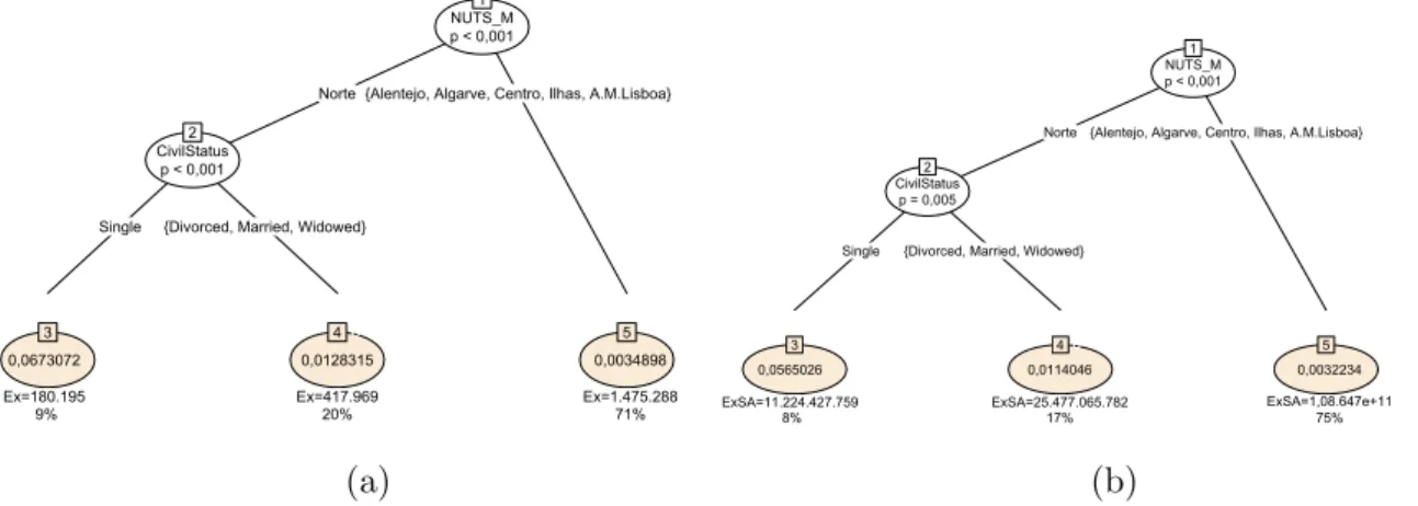
Variable Minimum 1st Median Mean 3rd Maximum Standard Total Sum

Quantile Quantile Deviation Assured

SA 2011 0,01 11.190 29.820 46.430 65.950 12.530.000 52.358 51×₁₀9

SA 2012 0,02 11.670 30.110 46.410 65.200 12.530.000 52.106 49×109

SA 2013 0,02 12.060 30.920 46.420 64.920 12.530.000 51.405 46×109

SA 2014 0,01 12.430 31.350 46.330 64.600 12.530.000 50.438 44×109

3.3

Exposed to risk

The concepts from Section 2.1 will now be used as the risk exposure of each person in the portfolio is calculated. The real age of the insured persons and an actual/actual base of calendar will be considered.

First, it was decided that the mortality graduation would be based on the insured lives and not on the policy participants, since one person can have more than one policy. As such, the same person, across all policies where he or she is insured, should only contribute to the risk exposure once per period of time.

Furthermore, the sum assured of each policy will be assumed to have changed at most once a year, with the start of each civil year. As such, our risk exposure calculation should be broken down by civil year, to make it possible to link the right sum assured to each period of time. We will now give an example.

Consider a person who was insured for the whole of 2011 and turned 50 on 01/07/2011. Following equation 2.1.1, this person will have

E₄₉= #days exposed risk(age49) #days year(2011) =

181

365, E50=

#days exposed risk(age50) #days year(2011) =

184 365.

Consider now that the same person had another policy in force from 01/08/2011 to 31/12/2011. If E_x was calculated without taking into account the person’s policies as a whole, we would have arrived to the conclusion that for 2011

E49=

181

365, E50=

184 + 153

365 =

337 365.

As such, that person would have counted twice for age 50 during the period of 01/08/2011 to 31/12/2011, which wouldn’t be coherent with our previous decision. Since the period in force of the second policy overlaps with that of the first policy, the correct result is

E49=

181

As stated in Subsection 2.1.1, we will be studying the mortality rates weighted by sum assured, which requires the weighted risk exposure, given by equation 2.1.3.

Continuing with the previous example, assume the first policy had 2.500_BC of sum assured and the second had 50.000BC. For the period of 01/01/2011 to 01/08/2011, the

sum assured was 2.500BC. For the period of 01/08/2011 to 31/12/2011, it was 2.500BC +

50.000BC = 52.500BC since the person was covered by both policies. Hence:

E₄₉SA = 181

365⇥2.500 = 1.240; E

SA

50 =

184

365⇥2.500 + 153

365⇥50.000 = 22.220.

Regarding the number of deaths at a given agex,dx, considering once again that a single

person could have multiple policies and, as such, a death claim in multiple polices, care had to be taken not to count the same person’s death more than once when calculating the mortality rates. For the mortality rates weighted by sum assured, the sum of the sums assured over all policies for which a death was reported will be used asdSA_x .

In order to perform the calculations previously explained, an algorithm was created to transform the data into a form where the exact risk exposure and number of deaths for any segment of the portfolio would be easily calculated. The objective was to break a policy’s (date of issue, end date) interval into smaller sub-intervals where there were no changes in age or sum assured.

The algorithm is explained in pseudo-code in Appendix B. The result was a data set with 3.379.418 records for the 781.772 different insured lives with the following attributes: person key, gender, civil status, NUTS M, Ex, age, ExSA, claim, SA Claim.

3.4

Mortality rates

In this section, we’ll look at the crude mortality rates (weighted and not) by age for the portfolio in study, first over all insured lives and then separated by each of the personal explanatory variables available (gender, civil status and NUTS M).

The individual identifier (person key) was dropped and the variables Ex, ExSA, claim and SA Claim were summed grouped by the personal characteristics. This produced 2.877 different combinations. In order to keep the results significant, we limited our analysis between ages 20 (before that there were no deaths) and 80 (after that there is barely any exposure to risk), leaving 2.655 different cohorts.

This structure will be the basis for constructing the observed mortality rates. The remainder of this section will be divided into two perspectives, using the data aggregated by age, gender, civil status and NUTS M:

• Mortality rates: Given by equation 2.1.2, where d_x and E_x are, respectively, the number of claims (field Claim) and the risk exposure (field Ex) for age x.

for age x.

Throughout this section, both approaches will also be compared via the formula

r =mean ✓

˜ q_xSA

˜ qx

◆

, (3.4.1)

where ˜qx and ˜qxSA are the observed values of qx and qxSA which are bigger than zero

(otherwise, the ratio would not be computable). The mean of the ratio is calculated grouped by the explanatory variable in analysis. The results of this value r provide a notion of how much higher (or lower)qx is than qxSA, on average.

3.4.1 Overall mortality rates

• Mortality rates: In Figure 3.4 we can see the mortality rates for the portfolio over ages 20 to 80. It resembles a slow growing exponential curve, which picks up at around age 65.

• Weighted mortality rates: In Figure 3.4, it’s possible to see the overall mortality rates for all ages weighted by sum assured. The behaviour is similar that of the traditional rates except that the growth with age seems to accelerate later.

Comparing the two approaches (Figure 3.4), it seems like qx is higher than qSAx for the

most part, especially for older ages. As a matter of fact, calculating r as stated before, qSA_x is on average 86% of q_x.

Figure 3.4: Overall mortality ratesversus mortality rates weighted by sum assured

3.4.2 Mortality rates by gender

• Mortality rates: Figure 3.5 (a) shows the mortality rates for the portfolio for male

versus female insured lives. From visual inspection of these plots, it seems like the female mortality rates are lower than the males’ for younger ages but then become higher after age 70.

Comparing the two approaches (plots have the same scale), the weighted rates seem lower. Calculating the mean of the ratio between the values (r),q_xSA is on average 93% ofqx for

females and 81% for males.

(a) (b)

Figure 3.5: Mortality rates by gender: (a) traditional; (b) weighted.

3.4.3 Mortality rates by civil status

• Mortality rates: Figure 3.6 (a) has the mortality rates divided by civil status. For this segmentation, it’s harder to draw conclusions given that there are more possible values for the explanatory variable.

• Weighted mortality rates: Values are plotted in Figure 3.6 (b), where once again no clear conclusions are possible.

Comparing the two approaches, it’s hard to say visually which one yields higher mortality rates. Calculating the ratio r, q_xSA is on average: 87% of qx for divorced people; 91%

of q_x for married people; 77% of q_x for singles; 108% of q_x for widowed people. In the case of widowed lives, the traditional mortality rates are for the first time higher than its weighted counterpart.

(a) (b)

3.4.4 Mortality rates by NUTS M

• Mortality rates: Finally, Figure 3.7 (a) shows the different mortality rates according to NUTS M of residence.

• Weighted mortality rates: Figure 3.7 (b) has the weighted mortality rates.

Trying to reach conclusions about the two approaches visually is pointless. Comparing the two through the mean ratior,q_xSA is on average: 100% of qx for Alentejo; 88% of qx

for Algarve; 86% ofqx for Lisboa; 96% ofqx for Centro; 80% ofqx for Ilhas; 75% ofqx for

Norte.

(a) (b)

Figure 3.7: Mortality rates by NUTS M: (a) traditional; (b) weighted.

Comparing the values of the mortality ratesversusthe weighted mortality rates through-out, for most segments, qSA_x is lower than qx, which is in line with the idea that people

with higher sums assured are wealthier and hence healthier, leading to longer lives.

3.5

Training and test sets

As discussed in Section 2.2, a training and a test set were used. The training set was composed of 80% of the insured lives in the data set (624.880) and the remaining 20% (156.220) as the test set. Note that this division was made over the number of unique insured lives and not the number of policyholders, so as to be coherent with the exposure and claim calculations.

In order to have a similar composition over the available explanatory variables of the training and test sets, compared to the original data set, stratified sampling was used, instead of directly doing a random sample of 80% of the insured lives. This is meant to avoid the risk of over-representing one segment of the population in the training set and under-representing it in the test set, orvice-versa.

Chapter 4

Results

In this chapter, the models of Section 2.2 will be applied to the training set. In the first four sections, the details and results of the application of each model will be presented, always divided by the two approaches of this thesis: (traditional) mortality rates and mortality rates weighted by sum assured. In the last Section (4.7), the models will be compared between them, using the test set to calculate the error.

Furthermore, recall r, as defined in equation 3.4.1. The results of this value will provide an idea of how much higher (or lower) the estimated qx is than the estimated

qSA_x , on average, for each model. Given that for some of the models the traditional and weighted mortality rates are grouped in different ways, the ratio r is only comparable for the overall (ungrouped) rates. These calculated values will be comparable to the ratio for the crude rates in Subsection 3.4.1, which was 86%.

4.1

Gompertz’s law

As stated in Subsection 2.2.1, the observed mortality rates were fit to the curve in equation 2.2.1. The two parameters in the equation were determined using the nls function from R, which calculates the nonlinear (weighted) least-squares estimates of the parameters of a nonlinear model. The fitting was done separately for male and female insured lives.

• Mortality rates: The fitting resulted in the curves bellow, visible in Figure 4.1 (a). Looking at the plot of the curves, one can see that the female curve grows much faster than the male curve for ages over 70, like for the crude mortality rates (Figure 3.5 (a)).

ˆ qx=

8 <

:

1 exp 5,08⇥10−10

⇥exp(0,26x) , Gender=f emale 1 exp 2,52⇥10−6

⇥exp(0,14x) , Gender=male

• Weighted mortality rates: The final curves are given by the formula bellow, plotted in Figure 4.1 (b). Again, replicating the behaviour of the crude mortality rates (Figure 3.5 (b)), the female curve exceeds the male curve for ages over 70.

ˆ qSA_x =

8 <

:

1 exp 2,49⇥10−10

⇥exp(0,27x) , Gender=f emale 1 exp 15,32⇥10−6

(a) (b)

Figure 4.1: Fitted curves for mortality rates- Gompertz’s law: (a) traditional; (b) weighted.

For this model, ˆqSA_x is on average 62% of ˆq_x.

4.2

Empirical approach

By this approach, the observed mortality rates were fit to the curve in equation 2.2.2. Again, the fitting was done separately for male and female insured lives and the parameters were determined using the nls function from R.

• Mortality rates: The fitting resulted in the curves in Figure 4.2 (a). From visual inspection, the male and female curves are indistinguishable up to around age 50. At this point, the male curve starts to exceed the female and the gap grows bigger up to age 70, where the curves intersect again and from that point on the female rates start to surpass the male ones.

ˆ qx=

8 <

:

3,57⇥10−10

⇥exp(0,29x), Gender=f emale 4,06⇥10−₁₀

⇥exp(0,12x), Gender=male

(a) (b)

Figure 4.2: Fitted curves for mortality rates- empirical approach: (a) traditional; (b) weighted.

in Figure 4.2 (b). Looking at the plot, the maximum value for this approach is reached at around 0,3 whereas for the previous model (Gompertz’s law), it was 0,5.

ˆ qSA_x =

8 <

:

3,20⇥10−12

⇥exp(0,32x), Gender=f emale 8,35⇥10−10

⇥exp(0,17x), Gender=male

For this approach, the estimated weighted mortality rates are on average 39% of the estimated traditional mortality rates.

4.3

Standard tables

The graduation using standard tables, as stated in Subsection 2.2.3, made use of the Swiss tables GKF80, GKM80, GKF95 and GKM95. These tables were adjusted to the data by gender, i.e., female data was adjusted to GKF80 and GKF95 and male data to GKM80 and GKM95. The formula in equation 2.2.3 was used and the function lm from R, which fits linear models, was utilised to find the parameter.

• Mortality rates: The application of this model resulted in (Figure 4.3 (a)):

– Using the 80 series: ˆqx=

8 <

:

2,82⇥GKF80x, Gender=f emale

0,56⇥GKM80x, Gender=male

;

– Using the 95 series: ˆqx=

8 <

:

1,87⇥GKF95x, Gender=f emale

0,74⇥GKM95x, Gender=male

.

(a) (b)

Figure 4.3: Fitted curves for mortality rates- standard tables: (a) traditional; (b) weighted.

The high value of the parameter for female data is due to the high values of the observed mortality rates for females over 70 in our data (see Figure 3.6 (a)). These are mostly outliers from a specific policy that existed for a year and was not renewed because of its unprofitable results. As a matter of fact, running the fitting process over the training lives under 70 years old, the results become:

– Using the 80 series: ˆq_x= 8 <

:

0,34⇥GKF80x, Gender=f emale

0,34⇥GKM80x, Gender=male

– Using the 95 series: ˆq_x= 8 <

:

0,20⇥GKF95x, Gender=f emale

0,48⇥GKM95x, Gender=male

.

• Weighted mortality rates: Graduation using the GK80 and GK95 standard tables resulted in the formulas bellow and Figure 4.3 (b).

– Using the 80 series: ˆq_xSA= 8 <

:

2,59⇥GKF80x, Gender=f emale

0,55⇥GKM80x, Gender=male

;

– Using the 95 series: ˆq_xSA= 8 <

:

1,70⇥GKF95x, Gender=f emale

0,69⇥GKM95x, Gender=male

.

As with the traditional rates, the unusually high value of the parameter fit to the female training data is due to the high weighted mortality rates at advanced ages (as can be observed in Figure 3.6 (b)). Fitting the data to the standard tables for lives under 70, the results become:

– Using the 80 series: ˆq_xSA= 8 <

:

0,31⇥GKF80x, Gender=f emale

0,36⇥GKM80x, Gender=male

;

– Using the 95 series: ˆq_xSA= 8 <

:

0,18⇥GKF95x, Gender=f emale

0,50⇥GKM95x, Gender=male

.

For the 80 series, ˆq_xSA is on average 93% of ˆqx. This is corroborated by the fact that

the weighted rates are adjusted by a smaller percentage of the standard tables than the traditional rates. For the 95 series,r is 92%.

4.4

GLM

Considering the definition of GLM given in Subsection 2.2.4 the distribution of Y was assumed to be Bernoulli with mean µ. Furthermore, the complementary log-log link functionη=cloglog(µ) =log( log(1 µ)) was used. Hence,µ= 1 e−eη

. Several other link functions were tried before deciding to use the complementary log-log function, which presented the best results for the data in question.

As a first approach, for both the traditional and weighted mortality rates, the four available explanatory variables (age, gender, civil status and NUTS M) were included, with no interaction between them. From this starting point, considering the p-value of the estimated parameters, adjustments were made to the explanatory variables in order to have statistically significant results. Maximum likelihood estimation was then used to estimate the parameters, using an iteratively reweighted least squares algorithm, through the glm function from the software R (stats package).

• Mortality rates: The final model is given by the formula

ˆ

qx = 1 exp( exp( 2,00 + 0,02x+CS+N+G)),

– CS = 8 > > > > > > < > > > > > > :

0, Civil Status=divorced 1,06, Civil Status=married

0,96 Civil Status=single 1,27 Civil Status=widowed

;

– N = 8 > > > < > > > :

0, N U T S M =Lisbon

1,31, N U T S M =Alentejo

0,60, N U T S M 2{Algarve, Ilhas, Centro, N orte} ;

– G= 8 <

:

0, Gender=f emale 0,36, Gender=male

.

No visual representation of this model is available since there are 24 possible com-binations of the explanatory variables gender, civil status and NUTS M.

• Weighted mortality rates: Coincidently, the exact same model was achieved for the weighted mortality rates as for the traditional rates. As such, ˆqSA_x = ˆq_x and the equations are omitted. No particular reason was found as to why the models coincided.

Given that the models coincided,r is obviously 100%.

4.5

Regression trees

In this section, models explained in Subsection 2.2.5 will be applied. However, unlike the previous applications in this chapter, for the tree generating algorithms, the explanatory variable age was not included because initial tests showed that it was such an important variable when modelling mortality that the first split was always done with it and at around age 70. This lead to a large majority of the data set being grouped into the same branch, which wasn’t a useful conclusion. As such, following Guoet al.(2002), the insured lives’ ages were not included to generate the trees. Age is is included afterwards to model the mortality of the persons that fit in each node of the generated trees, in Section 4.6.

4.5.1 CART

CART (see 2.2.5.1 ) is the basis for the rpart function from the software R (package rpart), which we used to obtain the results presented bellow. Details of this function can be found in Therneauet al. (2015). The minimum node size used was the default, 20.

Looking at the results from the tree, one might think that despite the age not being provided as an explanatory variable to the algorithm, the choices it made were conditioned by the age of the population that fell within each sub-division, acting as a proxy. However, if we calculate the average age within each leaf (weighted by the risk exposure and for the training data) the results are (from left to right hand-side leafs): 44, 46, 38 and 38 years old. As such, the leaf with the highest average age is the one representing the non-single people from Norte, which has a significantly lower mortality rate estimate than that for the single women from Norte, who are on average 8 years younger.

In Figures 4.4 and 4.5 the shaded boxes have the estimates for the mortality rates of each leaf, bellow each is the total risk exposure of the insured lives in the node (in the training set) and its weight on the overall risk exposure of the training set.

(a) (b)

Figure 4.4: Fitted model for mortality rates - CART: (a) traditional; (b) weighted.

• Weighted mortality rates: Figure 4.4 (b) shows that the results for the weighted and traditional mortality rates using CART are the same, in terms of explanatory variable splits, except that for the weighted mortality rates the gender was not considered important enough.

As with the traditional mortality rates, we calculated the average age within each leaf (weighted by the weighted risk exposure and for the training data) and the results are (from left to right hand-side leafs): 42, 44 and 37 years old. Again, we can then see that there is no evidence that the algorithm is using the available explanatory variables as a proxy for the age.

As would be expected, the predicted values for the weighted rates are lower than for the traditional ones. As a matter of fact, for CART, ˆq_xSA is on average 93% of ˆqx.

4.5.2 Conditional inference trees

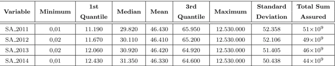
• Mortality rates: Figure 4.5 (a) shows the tree grown by the conditional inference trees algorithm. Once again, mortality for Norte is considered to be significantly different from the remaining values of NUTS M. As with CART, for insured lives from Norte, the algorithm goes on to divide between singles and the remaining civil status. It does not however consider gender important enough to differentiate the estimates. Notice that for nodes where splits are made (using the explanatory variables civil status and NUTS M) independence tests from the response variable (qx) had p-values under 0,001.

Looking at the average weighted age per leaf (for the training data), this will be the same as in the tree generated by CART except that the last split doesn’t occur but since the average age was 38 in both leafs, the average for that part of the population will also be 38. As such, the weighted average is (from left to right): 44, 46 and 38 years old. Again, no evidence was found that the algorithm was using the available explanatory variables as a proxy for age.

NUTS_M

p < 0,001

1

Norte{Alentejo, Algarve, Centro, Ilhas, A.M.Lisboa}

CivilStatus p < 0,001

2

Single {Divorced, Married, Widowed}

3 4 5

0,0673072 0,0128315 0,0034898

Ex=180.195 Ex=417.969 Ex=1.475.288

9% 20% 71%

NUTS_M p < 0,001 1

Norte {Alentejo, Algarve, Centro, Ilhas, A.M.Lisboa}

CivilStatus

p = 0,005

2

Single {Divorced, Married, Widowed}

3 4 5

0,0565026 0,0114046 0,0032234

ExSA=11.224.427.759 ExSA=25.477.065.782 ExSA=1,08.647e+11

8% 17% 75%

(a) (b)

Figure 4.5: Fitted model for mortality rates- conditional inference tree: (a) traditional; (b) weighted.

• Weighted mortality rates: Figure 4.5 (b) shows the tree grown for the weighted mortality rates. The splits made are the same as for the traditional mortality rates. In this tree, the NUTS M explanatory variable’s split is done due to the independ-ence test from the response variable (qSA

x ) having p-value under 0,001 and for the

civil status explanatory variable the p-value is 0,005. Though enough to reject the hypothesis of independence and create a split, it indicates that, according to this algorithm, there is a stronger link between the traditional mortality rates and civil status than between the weighted mortality rates and the same explanatory variable. In this case, the average weighted age per leaf will be exactly the same as with CART (42, 44 and 37 years old, from left to right) and we arrive at the same conclusion that the other variables are not being used as a proxy for age.

4.5.3 Random forests

To implement the random forests algorithm (explained in Subsection 2.2.5.3), the random-Forest function from R (package randomrandom-Forest) was used, details of which can be found in Liaw and Wiener (2002). For this model, the default number of trees for the randomForest function was used: 500. Tests were made regarding generating up to 100.000 trees but the results were not significantly different.

• Mortality rates: Figure 4.6 (a) shows the results of the Random Forest algorithm for the training set. The plot has only 48 points because this is how many different combinations of (civil status, NUTS M, gender) there are in the training data. As before, age is not taken into account, so for each combination of these characteristics, there is an unique estimated value. Looking at the plot, one sees that the male rates are most of the times higher than the female rates, which is to be expected. However, the inverse occurs and is exceptionally visible for the single people from Norte. This is in line with the conclusions from the other tree generating algorithms.

(a) (b)

Figure 4.6: Estimated mortality rates using the random forest algorithm: (a) traditional; (b) weighted.

• Weighted mortality rates: Figure 4.6 (b) shows the estimated weighted mortality rates for the training set, which exhibits the same overall behaviour as the traditional rates, although at a smaller scale (here, the maximum vale for the rates is at around 0,04 whereas for the traditional rates it’s at around 0,05).

For this approach, the estimated weighted mortality rates are on average 89% of of the estimated traditional mortality rates.

4.6

Hybrid models

4.6.1 CART and Gompertz’s law

• Mortality rates: Recalling Figure 4.4 (a), CART generated a tree with four leafs. Fitting Gompertz’s law to the force of mortality of the lives in each leaf results in the curves bellow, Figure 4.7 (a). Looking at the plot, one seems that the curve with the the highest rates is the one corresponding to leaf 4, which is in line with the results from CART.

ˆ qx= 8 > > > > > > < > > > > > > :

1 exp 4,49⇥10−5_{⇥exp(0,09x) , leaf= 1 (N 6=N orte)}

1 exp 6,55⇥10−9_{⇥exp(0,23x) , leaf= 2 (N =N orte ^CS6=single)}

1 exp 4,26⇥10−7_{⇥exp(0,17x) , leaf= 3 (N =N orte ^ CS=single ^ G=male)}

1 exp 2,98⇥10−7_{⇥exp(0,20x) , leaf= 4 (N =N orte ^ CS=single ^ G=f emale)}

(a) (b)

Figure 4.7: Fitted curves for mortality rates in each leaf- CART and Gompertz’s law: (a) traditional; (b) weighted.

• Weighted mortality rates: According to Figure 4.4 (b), CART generated a tree with three leafs. Fitting Gompertz’s law to the force of mortality of the lives in each leaf results in the curves bellow, Figure 4.7 (b). Visual inspection of the plot shows that the curves with lowest to highest mortality rates (1 to 3) are in the same sequence as the lowest to highest estimates in the tree.

ˆ qSA_x =

8 > > > < > > > :

1 exp 5,68⇥10−5

⇥exp(0,09x) , leaf = 1 (N 6=N orte) 1 exp 3,25⇥10−9

⇥exp(0,24x) , leaf = 2 (N =N orte ^CS6=single) 1 exp 1,96⇥10−7

⇥exp(0,26x) , leaf = 3 (N =N orte ^ CS=single) For this approach, ˆq_xSA is on average 100% of ˆqx. The ratio between the estimates is

100% only on average, it fluctuates point-wise.

4.6.2 CART and empirical approach

ˆ qx=

8 > > > > > > < > > > > > > :

6,07⇥10−5

⇥exp(0,07x), leaf = 1 (N 6=N orte) 2,15⇥10−11

⇥exp(0,29x), leaf = 2 (N =N orte ^CS6=single) 8,96⇥10−7

⇥exp(0,16x), leaf = 3 (N =N orte ^ CS =single ^ G=male) 2,71⇥10−6

⇥exp(0,16x), leaf = 4 (N =N orte ^ CS =single ^ G=f emale)

(a) (b)

Figure 4.8: Fitted curves for mortality rates in each leaf- CART and empirical approach: (a) traditional; (b) weighted.

• Weighted mortality rates: The final model is given by the formula bellow, see Figure 4.8 (b).

ˆ qSA_x =

8 > > > < > > > :

7,78⇥10−5

⇥exp(0,07x), leaf = 1 (N 6=N orte) 2,40⇥10−13

⇥exp(0,35x), leaf = 2 (N =N orte ^CS6=single) 1,02⇥10−8

⇥exp(0,23x), leaf = 3 (N =N orte ^ CS =single)

Like in the previous subsection, the sequence of lowest to highest mortality rates es-timates (both traditional and weighted) in the tree is the same as in the hybrid models. For this model, ˆq_xSA is on average 88% of ˆqx.

4.6.3 CART and GLM

For this hybrid model, instead of fitting a GLM model to each of the leafs of the tree, a similar approach to Guoet al. (2002) was adopted, using only the first split of the tree to divide the insured lives and then the remaining splits to determine which variables would go into the GLM and how. After generating a first model in this manner, the p-value of the estimated parameters was observed and adjustments were made in order to have statistically significant results.

ˆ q_x=

8 <

:

1 exp( exp( 2,24 + 0,03x+CS)), N U T S M =N orte 1 exp( exp( 2,00 + 0,02x)), N U T S M 6=N orte ,

whereCS = 8 <

:

0, Civil Status2{divorced, widowed, married}

1,41, Civil Status=single

.

Figure 4.9: Fitted curves for mortality rates- CART and GLM

• Weighted mortality rates: As in Subsection 4.4, the exact same model is achieved for both the weighted mortality rates and the traditional rates. Hence, ˆq_xSA = ˆqx

and the equations and plot of these are omitted.

For this type of hybrid model, the curves per leaf present a very different behaviour from those of the previous two subsections, especially for the single people from Norte (the red curve), which is convex instead of concave. Still, this segment of the population has the highest mortality rates estimates, in line with the results from the tree. Contrary to the crude mortality rates, for these models there isn’t a faster growth after age 70. Given that the models coincided,r is obviously 100%.

4.6.4 Conditional inference trees and Gompertz’s law

• Mortality rates: Recalling Figure 4.5, the conditional inference trees algorithm gen-erated a tree with three leafs. Fitting Gompertz’s law to to the force of mortality of the lives in each leaf resulted in the curves bellow.

ˆ qx=

8 > > > < > > > :

1 exp 2,59⇥10−7

⇥exp(0,19x) , leaf = 1 (N =N orte ^CS=single) 1 exp 6,55⇥10−9

⇥exp(0,23x) , leaf = 2 (N =N orte ^CS6=single) 1 exp 4,49⇥10−5

⇥exp(0,09x) , leaf = 3 (N 6=N orte)

Figure 4.10: Fitted curves for mortality rates in each leaf- conditional inference trees and Gompertz’s law

• Weighted mortality rates: Since for the weighted mortality rates the trees generated by the algorithms CART and conditional inference trees coincide, so did this model. Hence, the results are exactly the same as in Subsection 4.6.1.

For this approach, ˆqSA_x is on average 100% of ˆqx. The ratio between the estimates is 100%

only on average, it fluctuates point wise.

4.6.5 Conditional inference trees and empirical approach

• Mortality rates: Fitting an exponential curve to the mortality rates of the lives in each of the four leafs identified by the conditional inference tree algorithm, results in the curves bellow and Figure 4.11

ˆ qx=

8 > > > <

> > > :

1,81⇥10−6

⇥exp(0,16x), leaf = 1 (N =N orte ^CS =single) 2,15⇥10−11

⇥exp(0,29x), leaf = 2 (N =N orte ^CS 6=single) 6,07⇥10−5

⇥exp(0,07x), leaf = 3 (N 6=N orte)