The Effect of the Welfare Factor on Large Social Welfare Numbers*
Diana Vaz de Lima
PhD in Accounting Sciences from the Multi-institutional and Inter-regional Graduate Program in Accounting Sciences - University of Brasília / Federal University of Paraíba / Federal University of Rio Grande do Norte
E-mail: [email protected]
Marcelo Driemeyer Wilbert
Professor, Department of Accounting and Actuarial Sciences of the University of Brasilia E-mail: [email protected]
José Matias Pereira
Post-doctoral Professor of the Multi-institutional and Inter-regional Graduate Program in Accounting Sciences - University of Brasília / Federal University of Paraíba / Federal University of Rio Grande do Norte
E-mail: [email protected]
Edilson Paulo
Professor of the Multi-institutional and Inter-regional Graduate Program in Accounting Sciences - University of Brasília / Federal University of Paraíba / Federal University of Rio Grande do Norte
E-mail: [email protected]
Received on 12.23.2011 - Accepted on 1.2.2012 - 2nd version accepted on 6.29.2012
ABSTRACT
The welfare factor was introduced in 1999 by Act 9876 to promote a balance between the revenues and expenditures of the General Social Welfare System - GSWS. However, since its inception, it has been the target of criticism, and its abolition is often discussed. Given the importance of understanding the extent to which the introduction of the factor changed the financial structure of Brazilian social welfare and because limited research supports discussions on the retention or removal of the welfare factor, this study aims to analyze the effect of the welfare factor on large social welfare numbers. To that end, stationarity tests were performed to decide which model to use. Then, the structural breakdown of the data was tested, and an analysis was performed using an autoregressive model with trends to verify if the welfare factor variable (dummy) affected the series "Net Revenue", "Social Welfare Benefits Expenditure" and "Expenditure on Pensions by Contribution Period." The supporting monthly data were collected from the historical database of the Infologo Social Welfare Statistical Yearbook (Anuário Estatístico da Previdência Social - AEPS) from January 1988 to April 2011 for the first two variables and from January 1993 to August 2011 for the third. The results indicate that the implementation of the welfare factor has not been able to reverse the trend of higher growth of expenditures relative to revenue, thus confirming the expectation that social welfare finances will remain in deficit. For "Expenditure on Pensions by Contribution Period," since the implementation of the welfare factor, a slowdown in the growth trend of benefit payments has occurred. However, as this mode corresponds to only a portion of the total benefits paid, while acknowledging that the factor provided savings to the public coffers, its implementation has been unable to promote a balance between revenues and expenditures for the GSWS.
Keywords: Welfare Factor. Social Welfare. Brazil.
1 INTRODUCTION
Since its deployment, the welfare factor has been the target of opposition, mainly from organizations re-presenting the rights of workers and retirees who feel harmed by the reduction in social welfare benefits. At-tempts have been made to abolish the factor, including Bill 3.299/08, which was vetoed by the President in June 2010 despite having been approved by both houses of Congress.
Among the negative aspects, Oliveira, Ferreira and Car-doso (2000) emphasize that, although it contains actuarial elements (life expectancy, years of contribution and retire-ment age), the welfare factor is not based on actuarial crite-ria (equality between the expected present value of contri-butions and the expected present value of benefits) and is completely arbitrary.
According to the authors, there is no pre-determined and uniform discount rate for the various ages and con-tribution periods, which creates uncertainties and insecu-rities for the insured. Another important feature is related to the adopted mortality table, which was drafted by the Brazilian Institute of Geography and Statistics (Instituto Brasileiro de Geografia e Estatística - IBGE) and features technical, operational and legal problems (Oliveira, Ferrei-ra, & Cardoso, 2000).
The mortality table drafted by IBGE by the General Social Welfare System (GSWS) was adopted with the publication of Decree no. 3.266/1999, which is based on the complete mortality table for the total Brazilian population and considers a single national average for both sexes.
By studying the mortality of retired elderly of the GSWS, Souza (2009) observed that the IBGE life ex-pectancy curve for males is very close to the GSWS curve; however, this curve is lower for females. Thus, the recommendation is that "the use of mortality cur-ves should always consider the peculiarities of the stu-died population, to provide more reliable calculations" (Souza, 2009, p. 35).
However, Oliveira, Ferreira and Cardoso (2000) comment that, among the positive aspects, the welfare factor allows the insured to opt for particular retire-ment conditions, combining age, contribution period and value. This aspect also severely penalizes early re-tirement and delayed rere-tirement awards, although the benefit amount cannot exceed 100% of the GSWS sala-ry-benefit cap.
These aspects can be seen in the analysis of results of the welfare factor law from 1999 to 2004, which was per-formed by technicians of the Institute of Applied Econo-mic Research (Instituto de Pesquisa EconôEcono-mica Aplicada - IPEA). The data indicate that the welfare factor has rai-sed the pension age and contribution period and reduced
the value of the benefits of insured parties who retired after its introduction. Additionally, there is "a savings for welfare finances relative to the flow of granting Pensions by Contribution Period" (Delgado et al., 2006, p. 5).
Regarding the above and given the importance of un-derstanding to what extent the introduction of the factor changed the structure of social welfare finances, this study poses the following question: What were the effects of the implementation of the welfare factor on Brazilian large so-cial welfare numbers?
In this study, large numbers will be understood to mean the total social welfare contributions collected and the total social welfare benefits issued by the National Social Welfare Institute (Instituto Nacional de Seguri-dade Social - INSS), with additional analysis performed on benefit type 42 - retirement by contribution period - Organic Law of Social Welfare (OLSW), under which the welfare factor effectively falls.
The term "large numbers" is a reference to Table 1, which is an integral part of the Boletim Estatístico do Ministério da Previdência Social [Statistical Bulletin of the Ministry of Social Welfare], has been published for more than 15 years and provides a monthly summary of data on social welfare benefits, INSS and population cash flow.
The objective of this study is to verify to what extent the welfare factor affects large social welfare numbers. In the analysis of the series "Net Revenue" and "Social Welfare Benefits Expenditure," the supporting monthly data were collected from the historical database of the Infologo Social Welfare Statistical Yearbook - (Anuário Estatístico da Previdência Social - AEPS) from January 1988 to April 2011.
To analyze the effect of the factor on the series "Ex-penditure on Pensions by Contribution Period," data were collected on benefit type 42 - pensions by con-tribution period of the Organic Law of Social Welfare (OLSW) - extracted from Infologo starting from Janua-ry 1993, when the information first became available.
The research approach is qualitative and quantitative. Considering its objectives, the research possesses explo-ratory characteristics and seeks to understand the phe-nomenon of implementation of the welfare factor and its effect on Brazilian social welfare finances.
2 THEORETICAL BASIS
2.1 General basis of the GSWS.
The Brazilian Social Welfare System has three bases: the General Social Welfare System, the Complementary Social Welfare System (open and closed) and the Special Social Welfare System.
The General Social Welfare System (GSWS), or general basic public welfare, is outlined in art. 201 of the 1988 Federal Constitution, which states that "So-cial welfare will be organized in the form of a general system of contributory nature and compulsory mem-bership, subject to criteria that preserve financial and actuarial equilibrium."
The GSWS is national in scope and applicable to all private sector workers, civil servants and incumbent pu-blic employees serving in existing posts not linked to the system itself. It is managed by the National Social Welfare Institute (Instituto Nacional de Seguridade Social - INSS), created by Decree no. 99.350/1990 and established as a governmental agency connected to the Ministry of Social Welfare.
The benefits granted by the GSWS mostly extend to the period of need. They cover pensions, death be-nefits, aid, family allowance and maternity benefits. The pension is a lifetime monthly payment that can be awarded based on age, contribution period, disability or special needs.
The welfare factor is applied by INSS when provi-ding pensions by contribution period (PCP) and pen-sions by age (continued provision of these benefits), the latter only being included in the calculation when its value increases.
The benefits of PCP can be classified into three ma-jor types: 42 - retirement by contribution period (OLSW – Organic Law of Social Welfare); 46 - retirement by special contribution time; and other PCP. Data analysis will be performed on the total social welfare benefits is-sued and the amounts paid on type 42 - OLSW pension by contribution period, under which the welfare factor effectively falls.
2.2 GSWS Financing Model
According to Iyer (2002), when a pension system is mo-deled, one of the main issues to be resolved is the method according to which it will be funded. The method of fun-ding means the arrangement by which the existence of a flow of resources will meet the costs of the system, as and when they occur.
According to the author, social welfare systems under the responsibility of national governments are assumed to have infinite duration, taking for granted that there will be a regular infinite flow of new entrants
in the future. As a result, methods of financing social welfare systems are based on the approach known as open-end funding, which considers the initial popula-tion and future entrants as a single group for this pur-pose (Iyer, 2002).
In Brazil, the financing method adopted in the GSWS is simple distribution. According to Pinheiro (2005), in this system, the benefit expenditures anti-cipated for a given year are allocated in the same year, without contributions being made before capitalization of the plan if the assumptions set out in the funding plan are met.
In practice, when using this method, the benefit cost rates (contribution aliquot) are fixed to obtain revenue for the year equivalent to the anticipated expenditures. That is, costs are "spread" among participants (Capelo, 1986).
Gushiken, Ferrari and Freitas (2002) state that the simple allocation system can also be called a "budgetary system" because the goal is to determine contributions to be collected to support the cost of benefit payments in a given period, with no provision for any reserves for future benefits. According to the authors, this type of financing proposes a pact between generations because the active insured (current generation) pay the benefits of the inac-tive (past generation).
Given the direct relationship between contributions received and benefit payments made, the simple allo-cation system is very sensitive to changes in demogra-phic factors such as any change in the age profile of the participant community as a whole. Using this method, more so than with other systems, the size of the com-munity is most important because it will ensure the sustainability of the fund.
According to data from the Social Welfare Statisti-cal Bulletin (MPS, 2011), in April 2011, pensions were paid to a total of 15.7 million Brazilians, at a total value of R$12.4 billion. The pensions by contribution period (PCP) reached a total value of R$5.8 billion, with a mean benefit of R$1,279.14. The PCP corresponds to 46.5% of total paid pensions (age, PCP and disability), as illustra-ted in Figure 1.
Figure 1 PCP as proportion of total pensions paid
Source: Boletim Estatístico da Previdência Social [Social Welfare Statistical Bulletin] April 2011 (MPS, 2011)
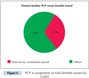
Figure 2 PCP as proportion of total benefits issued by GSWS
Source: Boletim Estatístico da Previdência Social [Social Welfare Statistical Bulletin] April 2011 (MPS, 2011)
1 According to the Ministry of Social Welfare (MPS) in Brazilian social welfare legislation, the contribution amount is the value of remuneration up to the GSWS cap under which the contribution aliquot falls (MPS, 1999). Tc × a
Es 100
(Id +Tc × a)
The implications of these results and the perception of the Brazilian government analysts that one of the main problems in the GSWS was the lack of correlation between the collection of contributions and payment of pension benefits led to the introduction of the welfare factor in 1999.
2.3 Implementation of the Welfare factor.
According to Amaro (2011), the promulgation of the Federal Constitution of 1988 led to two social wel-fare reforms: the first using Constitutional Amendment (CA) no. 20/1998 and the second using Amendments 45/2003 and 47/2005. However, neither of these refor-ms had a significant effect on the GSWS.
Two social welfare reforms were made, one in the FHC government and the other in the Lula government. Ho-wever, both have had an effect primarily on the civil service pension system and to a lesser extent on private pension schemes, leaving the conditions governing the
general social welfare system virtually unchanged (Ama-ro, 2011, p. 3).
However, the same author acknowledges that CA 20/1998 deconstitutionalized the rule for calculating benefits and constitutionalized the contributory nature of social welfare and its necessary financial and actuarial balance, thereby pa-ving the way for the enactment of Law no. 9,876/1999, which instituted the welfare factor (Amaro, 2011).
Law no. 9,876/1999 determined, among other things, the individual taxpayer's social welfare contributions and the calculation of benefits. This law introduced the welfare factor to promote a balance between revenues and expen-ditures of the General Social Welfare System (GSWS).
According to Afonso (2003, p. 29), the creation of the welfare factor had the objective of reducing early retire-ment and strengthening the link between the contributions and benefits of the GSWS. In practice, the welfare factor represented a type of toll, which reduced the benefit of insured parties who requested their pension to be moved forward. With the introduction of the factor, the pension calculation for each insured was based on certain basic pa-rameters and was determined according to equations 1 and 2 (MPS, 1999).
Sb= M × ƒ 1
where:
Sb = benefit amount
M = mean of the insured's highest 80% contribution
amounts1, calculated between July 1994 and time of
retire-ment, adjusted for inflation
ƒ = welfare factor
ƒ= × 1+ 2
where:
ƒ = welfare factor
Tc = time of contribution of each insured
a = contribution aliquot of the insured,
correspon-ding to 0.31 (constant, which represents 20% of employer contributions and always 11% of employee contributions)
Es = life expectancy of the insured at the time of
re-tirement, provided by the IBGE, considering only a single national mean for both sexes
Id = age of the insured at retirement date
According to the Social Welfare Report (MPS, 1999), the first part of the formula indicates that the reference period gradually extends and covers the en-tire working life of the insured entering the system after promulgation of the law. Thus, the basis for cal-culating benefits gradually corresponds to the mean income of the insured during the entire contribution period, making contributions and benefits issued equal in terms of value.
In adopting the new methodology, the law defined
Pension burden: PCP versus pensions
Age Disability Contribution period 16,8%
36,7%
46,5%
Pension burden: PCP versus benefits issued
Pensions by contribution period Others
60 60
n 60 - n
2 The authors excluded the work of Zorzin (2008), which they say addresses the relationship between social welfare and racial inequality. a transition period of 60 months, with gradual
imple-mentation of the welfare factor, according to the for-mula presented in Equation 3, which took effect in its entirety in 2004.
ƒn = ƒ × + 3
where:
ƒ
n = transition factor
ƒ = welfare factor, defined earlier
n = number of months from the date of enactment
of the law to the retirement date of the insured
In addition to the transition rule, in the implemen-tation of the welfare factor, a bonus of 5 years was ne-gotiated for the time of contribution for women and of 10 and 5 years, respectively, for kindergarten, elemen-tary and middle school teachers such that these perio-ds are added to the effective time of contribution that these categories exhibit in the calculation of the welfare factor (MPS, 1999).
2.4 Effects of the Welfare factor.
It appears that in correlating the contribution pe-riod and retirement age variables, the welfare factor affects collection of social welfare contributions (to the extent that the insured remains actively contributing to the system) and the amount of pension benefits is-sued (delaying the exit of the insured, who must stay in the labor market longer, thus delaying the insured’s demand for benefits).
The introduction of life expectancy of the insured in the calculation of the welfare factor, which is fundamental to plans with a simple allocation funding system, has proven even more relevant when analyzing the Brazilian popula-tion, which has undergone significant changes in its demo-graphic profile (IPEA, in 2010).
However, according to Delgado et al. (2006), when the effects of full implementation of the factor (end of the 60 month transition rule) and duration of the new life expectancy tables drafted by the IBGE were combi-ned in 2004, the factor law had a much more obvious restrictive effect on the calculation of remuneration of potential retirees and beneficiaries, which would ex-plain criticism of the model.
That said, it is perfectly understandable that the national representatives of the Workers' Central Union (Central Única dos Trabalhadores - CUT) and the Brazilian Con-federation of Retirees (Confederação Brasileira de Apo-sentados - Cobap) with seats on the CNPS, reflecting the demands of their members, have requested an assessment of the effects of the Welfare Factor Law. (Delgado et al., 2006, p. 8)
In the view of Fígoli and Ribeiro (2008), multiplying the contribution period by the aliquot should provide the number of months during which the insured
con-tributed to social welfare from their mean salary. Di-viding this number by the mortality rate balances the number of contributory months to the number of mon-ths of receiving the benefit, making the factor actua-rially fair.
However, the same researchers report that, by de-termining the mean period of future benefits using the same life expectancy for the entire Brazilian popula-tion, without considering the different mortality of va-rious population segments, the welfare factor ultimate-ly perpetuates inequalities between different segments of the population.
If specific life expectancies for each segment of the popu-lation were used when calculating the factor, the factor would increase for men and for people from the poorest states, as they have shorter life expectancies at the time of retirement. This fact indicates that the current system for calculating pension benefits favors women and states with a better quality of life (Ribeiro & Figoli, 2008, p. 51). For Giambiagi and Afonso (2009), for lower retirement ages, which correspond to shorter contributory periods, the factor is significantly less than 1, which would reduce the amount of pension. It should be understood that actuarial requirements partly covered in the welfare factor formula should also be incorporated in the pension calculation for those who retire by age.
Afonso and Lima (2011) note that despite the im-portance of creating the welfare factor, two important gaps in the literature on social welfare in Brazil are still present. One is related to the issue of distribution, in which the main focus is the distributional effects that social welfare systems can have, especially in
interge-nerational terms2, where individuals with different
characteristics (gender, age of entry into the labor ma-rket and retirement age, among others) may be affected differently by social welfare.
The second gap relates to the fact that some con-tributions do not explicitly consider the demographic risks (data on the probability of death for each age) as-sociated with the flows of contributions and receipts of social welfare benefits. According to the authors, these risks can be quite relevant, and their inclusion can make the models and results more accurate, thus providing information to social welfare policymakers (Afonso & Lima, 2011).
Varsano and Moura (2007, p. 332) report that two other factors seem to contribute to the social welfare de-ficit: the real increase in the minimum wage and the low dynamism of the Brazilian economy in the recent past. For minimum wage (MW), its increase affects both reve-nues and benefits issued; however, due to the very logic of the calculation of issued benefits, the pace of revenue growth is less than that of expenditures, "increasing the actuarial and financial imbalances and distortions from pension by contribution period."
Table 1 Evolution of readjustment of issued pension benefits 1995-2010
Period
Evolution of Minimum Evolution above Minimum
Min. Benefit Readjustment
INPC Inflation Index
Real INPC In-crease
Benefit Readjustment >MW
INPC Inflation Index
Real INPC Increase
1995-1998 85,71% 55,18% 19,68% 85,55% 71,52% 8,18%
1999-2002 53,85% 27,61% 20,56% 30,13% 27,67% 1,92%
2003-2006 75,00% 39,64% 25,32% 39,75% 38,58% 0,85%
2007-2010 45,71% 18,81% 22,65% 23,76% 18,81% 4,16%
1995-2010 628,57% 228,53% 121,76% 317,61% 260,54% 15,85%
Source: Informe Previdência Social [Social Welfare Report] June 2010 (MPS, 2010).
Table 2 Flow of GSWS Net Revenue and Benefit Payments 1988-2010
Consolidated Cash Flow of the INSS (In R$ 1,000.00)3
Exercise Net revenue Expenditure on Social Welfare Benefits Social Welfare Balance
1988 71.306.031 41.293.456 30.012.575
1989 70.623.797 44.106.410 26.517.387
1990 72.952.611 45.204.792 27.747.819
1991 65.579.029 47.399.186 18.179.843
1992 64.695.694 51.594.455 13.101.239
1993 73.517.400 69.413.554 4.103.846
1994 78.455.912 76.581.523 1.874.389
1995 94.243.866 94.995.791 - 751.925
1996 102.737.739 103.393.829 - 656.090
1997 106.270.882 113.657.017 - 7.386.135
1998 108.244.002 124.724.959 - 16.480.957
1999 108.497.056 129.228.905 - 20.731.849
2000 104.885.732 136.778.096 - 31.892.364
2001 120.863.089 145.492.185 - 24.629.096
2002 124.342.124 153.916.370 -29.574.246
2003 121.130.614 160.643.783 -39.513.169
2004 132.457.459 177.561.483 -45.104.024
2005 144.914.536 195.106.922 -50.192.386
2006 159.931.870 214.492.129 -54.560.259
2007 174.520.945 230.388.655 -55.867.710
2008 190.504.192 232.916.056 -42.411.864
2009 202.191.687 249.968.345 -47.776.658
2010 223.813.177 269.448.559 -45.635.382
Source: the author, based on annual data extracted from the Infologo historical database of AEPS from 1988-2010.
3 The values were corrected by the Accumulated INPC – base April 2011.
comment that the low growth of the GDP between 1994 and 2005 reduced the capacity for expansion of revenue: "between 1994 and 2005, the MW, responsible for the read-justment of most of the benefits, rose by 60% against a real increase in GDP of 30%" (Varsano & Moura, 2007, p. 332).
Supporting this interpretation, the data presented in the Social Welfare Report (MPS, 2010), covering the
period from 1995 to 2010, indicate that, compared with the National Index of Consumer Prices (NICP), which is the index officially used by the MPS to readjust issued pension benefits, the real increase of the minimum pen-sion was 121.76%. Benefits issued with values above the minimum wage had a real increase of 15.83% over the same period (Table 1).
Another important discussion is whether the de-ployment of the welfare factor could in fact promote a balance between revenues and expenditures because the
GSWS’s social welfare finances continue to show succes-sive deficits, as indicated in Table 2.
Despite the observance of successive deficits, studies indicate that the situation could be worse. To estimate the savings due to the welfare factor in the public accounts, Su-perti, Wu and Cruz (2011) developed an empirical
The INSS would cost more annually, approximately R$ 14 billion for those who applied for pensions from 2000-2009. This savings, however, does not consider that the insured may die before reaching life expectancy. By including the possibility of death, the government would spend approxi-mately R$10 billion annually, totaling almost R$450 billion at the end of the last year of life of the insured group who lived longer. This value represents a total expenditure of 35.5% if the factor was not used. However, it is noteworthy
that estimates for values and the budgetary cost reduction were based on inflation, while certain ranges of social wel-fare benefits had higher readjustments than the accumula-ted index of the period. Thus, the amount saved can chan-ge. (Superti, Wu, & Cruz, 2011, p. 13)
Given this perspective, the goal of this study is to unders-tand the effect of the welfare factor on large social welfare numbers since its introduction into social welfare finances.
3 METHODOLOGICAL PROCEDURES
3.1 Research Type and Method.
Because the objective of this study is to understand to what extent the introduction of the welfare factor has chan-ged the structure of Brazilian social welfare finances and to analyze its effect on large social welfare numbers, the rese-arch will be of the explanatory type.
Regarding technical procedures, because of the need to verify whether the welfare factor variable (dummy) affects the series "Net Revenue," "Expenditure on Social Welfare Benefits" and "Expenditure on Pension by Contribution Period," it will be reviewed using an autoregressive model with trends.
It should be noted that the objective is to study the change or absence of change in the behavior of these series based on the deployment of the welfare factor.
Keeping in mind the limitations mentioned in the li-terature regarding the use of time series, the tool was only used in this study for the purpose of measurement and not to make future projections.
The research approach is both qualitative and quanti-tative to allow for the understanding of the complexity of the nature of the welfare factor and uses bibliographical and documentary searches (qualitative) and analysis of the factor's effect by applying statistical tests (quantitative).
3.2 Sample Selection and Composition.
For the purposes of this study, the Infologo histori-cal database of the Social Welfare Statistihistori-cal Yearbook (Anuário Estatístico da Previdência Social - AEPS) was used, considering monthly data related to the net reve-nue from contributions and the amount of expenditure on social welfare benefits issued, covering the period from January 1988 to April 2011, and totaling 280 data points for each variable analyzed.
To analyze the effect of the welfare factor on bene-fits issued for type 42 - pension by contribution pe-riod OLSW (Organic Law of Social Welfare), data were analyzed for the period from January 1993 (when they first became available) to August 2011, totaling 224 data points for each variable analyzed.
The following variables were used in the study: "Net Revenue" (NR), "Social Welfare Benefits Expenditure"
(BE) and "Expenditure on Pension by Contribution
Pe-riod" (EPCP). The welfare factor variable (F) was added
to analyze the behavior of social welfare accounts before
and after its deployment, and the time variable (T) was
included to verify the trend of the time series.
The "Net Revenue" variable is the term used in INSS cash flow to represent the social welfare balance and cor-responds to actual revenues (bank collections, including escrow deposits, refunds and reimbursements) minus transfers to third parties (the value of social contribu-tions transferred to respective entities).
The variable "Social Welfare Benefit Expenditure" refers to social welfare benefits (pensions, benefits and financial aid) issued in the period, i.e., credits issued for payment of benefits that are active in the register.
With respect to the variable "Expenditure on Pensions by Contribution Period", there are currently three types being granted: 42 - Pension by contribution period OLSW (Organic Law of Social Welfare), 46 - Pension by special contribution period and other pensions by contribution period (57 and others). The study will focus on the be-nefits of pension by contribution period (PCP) of type 42, for which the welfare factor is applied.
For the methodology to be consistent throughout the period analyzed, the figures for net contributions reve-nue and the amount of expenditure on social welfare be-nefits issued were corrected by the accumulated INPC – based on April 2011. The figures for benefits issued for type 42 - pension by contribution period OLSW were corrected by the accumulated INPC – based on August 2011. This index measures the cost of living of families with incomes between one and six minimum wages, and the index is officially used by the INSS to readjust the social welfare benefits issued.
3.3 Development of Hypotheses and Definition
of Models Used.
Previously, statistical tests were applied to the series "Net Revenue," "Social Welfare Benefits Expenditure" and "Expenditure on Pensions by Contribution Period" to define the econometric model to be used to test whether the introduction of the welfare factor variable (dummy) changes the behavior of the series studied by technically analyzing the intercept and slope of the trend.
Figure 3 Net Social Welfare Revenue Jan. 1988 – Apr. 2011
4 ANALYSIS OF RESULTS
4.1 Net Revenue.
Figure 3 plots the "Net Revenue" series for social wel-fare contributions from January 1988 to April 2011 (280
months), with the values in Reais for April 2011 (infla-tion by INPC).
The Phillips-Perron unit root test indicates non-stationarity for random walk and non-stationarity for random walk with displacement. Moreover, the test allows us to reject the null hypothesis (less than 1% significance level) of the existence of a unit root for the random walk model with displacement around a stochastic trend.
Thus, based on the chart for the historical series "Net Revenue" and the Phillips-Perron stationarity test, the series should be modeled as stationary around a deterministic trend. In the model, today's revenue de-pends on a portion of yesterday's revenue and a com-ponent tied to the time variable. First, the evaluation of the autoregressive model with trend is performed as in Equation 4:
ALt= β0 + β1ALt-1 + β2T + ut 4
where:
ALt = “Net Revenue” of GSWS at time t
ALt-1 = “Net Revenue” of GSWS at time t-1
T = Time variable
Based on this model, the occurrence of a structural break in the data for the month of November 1999, the time of first deployment of the welfare factor, was tes-ted. As previously noted, due to the transition period,
application of the welfare factor occurred gradually over a period of 60 months, and it only went into full effect in 2004 and has remained in effect to the present day. However, both the Chow Breakpoint Test and the Chow Forecast Test indicate the occurrence of a structural bre-ak upon its implementation.
The next step was to estimate the model with the in-clusion of binary variables (dummy), representing the adoption of the welfare factor. Therefore, the welfare
factor variable (F) takes a value of zero in the months
when the welfare factor was not in force and takes a va-lue of 1 after the introduction of the factor. In addition, the estimation was made robust to heteroscedasticity (White's consistent covariances and standard errors), as in Equation 5:
ALt= β0 + β1.F + β2.ALt-1 + β3.T + β4.F.T 5
where:
ALt = “Net Revenue” of GSWS at time t
F = dummy variable referring to the welfare factor
(equal to 1 if with welfare factor or 0 if not)
ALt-1 = “Net revenue” of GSWS at time t-1
T = Time variable
jan/1988 oct/1988 jul/1989 apr/1990 jan/1991 oct/1991 jul/1992 apr/1993 jan/1994 oct/1994 jul/1995 apr/1996 jan/1997 oct/1997 jul/1998 apr/1999 jan/2000 oct/2000 jul/2001 apr/2002 jan/2003 oct/2003 jul/2004 apr/2005 jan/2006 oct/2006 jul/2007 apr/2008 jan/2009 oct/2009 jul/2010 apr/2011 35,0
30,0
25,0
20,0
15,0
10,0
5,0
0,0
Billions
of
Reais
for
Apr
2011
Table 3 Results of estimation of historical series “Net Revenue”
Variable Coefficient T statistic Probability (significance)
Constant 4,81X10⁹ 26.64317 0,0000a
Factor (dummy) -8,52X10⁹ -6.586019 0,0000a
Revenue Previous Period -0.005655 -0.112875 0.9102b
Time 30.349.846 10.65685 0,0000a
Time Factor* 48.679.621 6.989950 0,0000a
Observations:
1) The superscript (a) indicates statistical significance of less than 1%, and the superscript (b) indicates that the parameter was not significant. 2) R2 = 0,761094
3) Number of observations = 280.
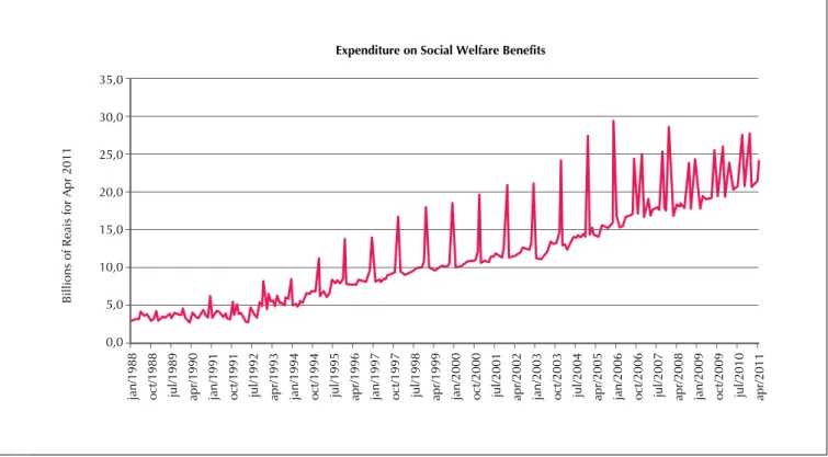
Figure 4 Expenditure on total social welfare benefits issued Jan 1988- Apr 2011 As observed in Table 3, the parameters associated
with the Factor dummy variable, the Time trend varia-ble and the interaction term (dummy Factor and Time) were strongly significant. The parameter associated
with the de-phased "Net Revenue" variable was not sig-nificant. The autoregressive model was stationary, and based on the Breusch-Godfrey test, it did not correlate with the other series.
Thus, based on the results, it appears that the imple-mentation of the welfare factor has changed the histori-cal series of "Net Revenue" for social welfare contribu-tions. This fact was proven by statistical tests, although implementation of the factor was not immediate and occurred over a given period.
Notably, the parameter associated with the Factor dummy variable has a negative sign, indicating that deployment of the welfare factor shifted the historical revenue series downwards. In contrast, the parameter associated with the interaction term Factor compared with Time had a positive sign, indicating that
deploy-ment of the welfare factor changed the trend by increa-sing the slope in this case. This steepening of the trend after the introduction of the welfare factor indicates that social welfare revenue achieved further growth from that point forward.
4.2 Expenditure on the amount of social welfare
benefits issued.
Figure 4 plots the expenditures on social welfare benefits issued from January 1988 to April 2011 (280 months) against the values in Reais in April 2011 (cor-rection by INPC).
35,0
30,0
25,0
20,0
15,0
10,0
5,0
0,0
Expenditure on Social Welfare Benefits
jan/1988 oct/1988 jul/1989
apr/1990 jan/1991 oct/1991 jul/1992
apr/1993 jan/1994 oct/1994 jul/1995
apr/1996 jan/1997 oct/1997 jul/1998
apr/1999 jan/2000 oct/2000 jul/2001
apr/2002 jan/2003 oct/2003 jul/2004
apr/2005 jan/2006 oct/2006 jul/2007
apr/2008 jan/2009 oct/2009 jul/2010
apr/2011
Billions
of
Reais
for
Apr
Table 4 Results of Estimation of the Expenditure using the Social Welfare Benefits Historical Series
Variable Coefficient T statistic Probability (significance)
Constant 1,96X10⁹ 9,663419 0,0000a
Factor (dummy) -5,20X10⁹ -4,024376 0,0001a
Expenditure Previous Period 0,012949 0,309776 0,7570b
Time 62.296.891 19,07461 0,0000a
Time Factor* 31.241.053 4,650856 0,0000a
Observations:
1) 1) The superscript (a) indicates statistical significance of less than 1%, and the superscript (b) indicates that the parameter was not significant. 2) R2 = 0,865233
3) Number of observations = 280.
Based on the Phillips-Perron test (unit root), the se-ries is non-stationary for random walk, stationary at 5% significance for random walk with displacement and stationary with less than 1% significance for random walk with displacement around a stochastic trend.
Thus, based on the data chart and the Phillips-Perron test, the series should be modeled as stationary around a deterministic trend. Expenditure on today's tax benefit is therefore modeled as a function of a por-tion of yesterday's expenditures and another porpor-tion associated with the time variable. First, an evaluation is performed of the autoregressive model with trends as in Equation 6:
DBt= β0 + β1.DBt-1 + β2.T + ut 6
where:
DBt = Expenditure on social welfare benefits of
GSWS issued at time t;
DBt-1= Expenditure on social welfare benefits of
GSWS issued at time t-1; T = Time variable.
Based on this model, the occurrence of structural breaks in the data was tested for the month of Novem-ber 1999, the time of first deployment of the welfare factor. As in the "Net Revenue" series, both the Chow Breakpoint Test and the Chow Forecast Test indicate
the occurrence of structural breaks in the series " Ex-penditure on Social Welfare Benefits " from the time of first deployment of the factor.
The next step was to estimate the model with the inclusion of binary variables (dummy) representing the adoption of the welfare factor. In addition, the esti-mation was made robust to heteroscedasticity (White's consistent covariances and standard errors), as in Equation 7:
DB
t= β0 + β1.F + β2.DBt-1 + β3.T + β4.F.T 7
where:
DBt = Expenditure on social welfare benefits of
GSWS issued at time t;
F = dummy variable referring to the welfare factor (equal to 1 if factor present and 0 if not);
DBt-1= Expenditure on social welfare benefits of
GSWS issued at time t-1; T = Time variable.
The parameters associated with the Factor dummy variable, the Time trend variable and the interaction term (dummy Factor and Time) were strongly signi-ficant. The parameter associated with the de-phased variable expenditures on social welfare benefits issued did not appear significant. Table 4 below presents the main results.
The autoregressive model appeared stationary, and based on the Breusch-Godfrey test, it did not correla-te with the other series. Thus, based on the results, it appears that the implementation of the welfare factor changed the historical series "Expenditure on Social Welfare Benefits" of the GSWS.
As in the "Net Revenue" series, in the estimation of the series "Expenditure on Social Welfare Benefits," the parameter associated with the Factor dummy variable had a negative sign, indicating that deployment of the welfare factor shifted the historical series of expenditu-res downwards.
In contrast, the parameter associated with the inte-raction term Factor compared with Time had a positive
sign, indicating that deployment of the welfare factor changed the trend by increasing the slope in this case. This increase in slope of the trend for the historical se-ries of expenditures on social welfare benefits issued indicates that growth in expenditures increased after the introduction of the welfare factor.
4.3 Expenditure on Retirement by Contribution
Period.
Figure 5 Expenditure on Pensions by Contribution Period Jan 1993 – Aug 2011
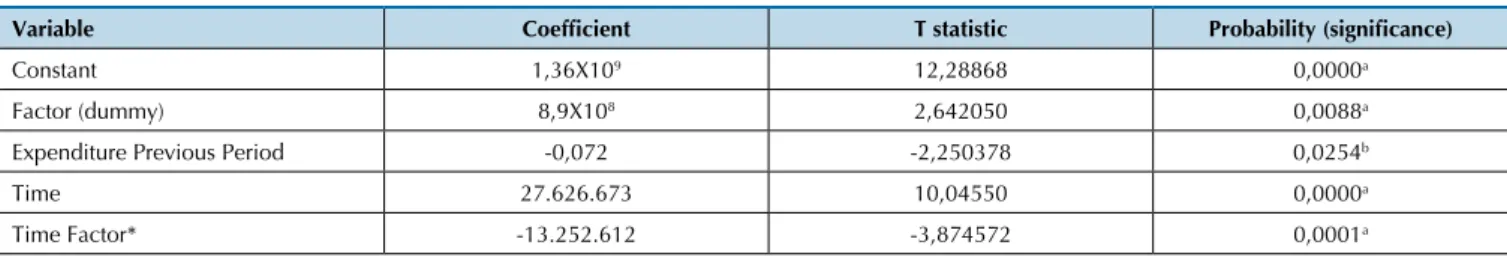
Table 5 Results of Estimation of the Expenditure using the Pensions by Contribution Period Historical Series
Variable Coefficient T statistic Probability (significance)
Constant 1,36X10⁹ 12,28868 0,0000a
Factor (dummy) 8,9X10⁸ 2,642050 0,0088a
Expenditure Previous Period -0,072 -2,250378 0,0254b
Time 27.626.673 10,04550 0,0000a
Time Factor* -13.252.612 -3,874572 0,0001a
Observations:
1) The superscript (a) indicates statistical significance of less than 1%, and the superscript (b) indicates a statistical significance of 2.5%. 2) R2 = 0.613194
3) Number of Observations = 224
Based on the Phillips-Perron test (unit root), the se-ries is stationary at less than 1% significance for random walk with displacement around a stochastic trend.
Thus, based on the data chart and the Phillips-Perron test, the historical series should be modeled as stationary around a deterministic trend. Therefore, the expenditures on pensions by contribution period are modeled as a function of a portion of yesterday's expenditures and another portion associated with the time variable. First, an evaluation is performed of the autoregressive model with a trend as in Equation 8:
DATCt= β0 + β1.DACTt-1 + β2.T + ut 8
where:
DPCPt= Expenditure on Pensions by Contribution
Period at time t;
DPCPt-1= Expenditure on Pensions by Contribution
Period at time t-1; T = Time variable.
Based on this model, the occurrence of a structural bre-ak in the data was tested for the month of November 1999, the first deployment of the welfare factor. As in the pre-vious series, both the Chow Breakpoint Test and the Chow Forecast Test indicate the occurrence of structural breaks in the series "Expenditure on Pension by Contribution
Pe-riod" from the time of first deployment of the factor. The next step was to estimate the model with the inclusion of binary variables (dummy), representing the adoption of the welfare factor. In addition, the esti-mation was made robust to heteroscedasticity (White's consistent covariances and standard errors), as in Equation 9:
DATC
t= β0 + β1.F+ β2.DACTt-1 + β3.T + β4.F.T 9
where:
DPCPt= Expenditure on Pensions by Contribution
Period at time t;
F= dummy variable referring to the welfare factor (equal to 1 where factor present and equal to zero whe-re not pwhe-resent);
DPCPt-1= Expenditure on Pensions by Contribution
Period at time t-1; T= Time variable.
The parameters associated with the Factor dummy varia-ble, the Time trend variable and the interaction term (dummy Factor and Time) were strongly significant. The parameter associated with the de-phased expenditures on pension by contribution period variable was significant at the 2.5% level of significance. Table 5 below presents the main results.
jan/1993 jul/1993 jan/1994 jul/1994 jan/1995 jul/1995 jan/1996 jul/1996 jan/1997
ju/1997
jan/1998 jul/1998 jan/1999 jul/1999 jan/2000 jul/2000 jan/2001 jul/2001 jan/2002 jul/2002 jan/2003 jul/2003 jan/2004 jul/2004 jan/2005 jul/2005 jan/2006 jul/2006 jan/2007 jul/2007 jan/2008 jul/2008 jan/2009 jul/2009 jan/2010 jul/2010 jan/2011 jul/2011
9,0
8,0
7,0
6,0
5,0
4,0
3,0
2,0
1,0
0,0
Pension by Contribution Period
Billions
of
Reais
for
Aug
Figure 6 Evolution of revenue, benefits and social welfare balance Jan 1988 – Apr 2011 The autoregressive model appeared stationary, and
based on the Breusch-Godfrey test, it did not correla-te with the other series. Thus, based on the results, it appears that the implementation of the welfare factor changed the historical series "Expenditure on Pensions by Contribution Period" of the GSWS.
In contrast to the "Net Revenue" and "Social Welfare Benefits Expenditure" series, the parameter associated with the Factor dummy variable had a positive sign, indicating that deployment of the welfare factor shifted the historical series of expenditures on PCP upwards.
More importantly, unlike the results for the previous series, the parameter associated with the interaction term, Factor T compared with Time, had a negative sign, indicating that deployment of the welfare factor changed the historical trend by decreasing the slope in this case. That is, the deployment of the welfare factor led to slower growth for expenditures on pensions by contribution period.
4.4 Comparative analysis: "Net Revenue"
compared with "Expenditure on Benefits
Issued" and "Expenditure on Pensions by
Contribution Period".
In the estimates for the "Net Revenue" and "Expen-diture on Social Welfare Benefits" series, both had a Factor dummy variable with a negative sign. However, the downward shift identified was larger for the "Net Revenue" series than for the "Expenditure on Social Welfare Benefits” series.
In the period before the introduction of the welfa-re factor, the slope of the variable twelfa-rend of the series "Expenditure on Social Welfare Benefits" was 105.3% greater than the slope of the variable trend for the "Net Revenue" series. Therefore, an indication that social welfare benefits payments exceeded the value of social welfare contributions revenue was already present.
Another finding was that the introduction of the welfare factor increased the slope of the trend in both contributions to revenue and expenditures on benefits issued. Moreover, the results demonstrate that the de-ployment of the welfare factor caused a major change in the trend for the "Net Revenue" series, which was 55.8% higher than the increase for the "Expenditure on Social Welfare Benefits" series. Even so, the slope of the trend for the "Expenditure on Social Welfare Benefits" series was greater than the slope of the trend for the "Net Revenue" series.
Based on the above results, from this analysis, it may be concluded that the implementation of the fare factor was able to change the trend of social fare revenue. However, the implementation of the wel-fare factor was not able to reverse the previous trend of higher growth in expenditure relative revenue, thus perpetuating the expectation that social welfare finan-ces will remain in deficit. Figure 6 presents the histo-rical evolution of the "Net Revenue" and "Expenditure on Social Welfare Benefits" series against the result of their difference (Social Welfare Balance).
35,0
30,0
25,0
20,0
15,0
10,0
5,0
0,0
-5,0
-10,0
-15,0
Revenue, Benefits and Social Welfare Benefits
Net Revenue Expenditure on Benefits Balance
Billions
of
Reais
for
Apr
2011
Afonso, L. E. (2003). Um estudo dos aspectos distributivos da previdência social no Brasil. 124 f. Tese de doutorado em Economia, Faculdade de Economia, Administração e Contabilidade, São Paulo, Brasil. Afonso, L.E., & Lima, D. de A. (2011). Uma análise dos aspectos
distributivos da aposentadoria por tempo de contribuição do INSS com o emprego de matemática atuarial. Revista Gestão & Políticas Públicas. 1 (2), 7-33.
Amaro, M. N. (2011, fevereiro). Terceira reforma da previdência: até
quando esperar? Centro de Estudos da Consultoria do Senado.
Textos para Discussão, 84. Recuperado em 23 junho, 2011, de http://www.senado.gov.br/senado/conleg/textos_discussao/TD84-MeirianeNunesAmaro.pdf.
Anuário Estatístico da Previdência Social Infologos. AEPS Infologo. (2011). Recuperado em junho, 2011, de http://www3.dataprev.gov.br/ infologo/.
Capelo, E. R. (1986). Fundos privados de pensão: uma introdução ao estudo
References
It is noteworthy that after the implementation of the welfare factor, the data referring to "Expenditure on Social Welfare Benefits" exhibit an increase in the slope of the trend, indicating an increase in the social welfare benefits issued. This result could indicate that the welfare factor was not able to discourage early re-tirement.
The above analysis considers social welfare benefits
issued in their entirety. When observing the behavior of the benefits of pension by contribution period, it was observed that the implementation of the welfare factor slowed the growth trend of the volume paid. However, as the payment of pensions by contribution period repre-sents only a portion of the total paid, as indicated earlier in Figures 1 and 2, this slowdown was not sufficient to change the overall trend of payment of benefits.
5 FINAL CONSIDERATIONS
The present study aimed to analyze the effect of the welfare factor on large social welfare numbers based on monthly data collected in the historical database of the Infologo Social Welfare Statistical Yearbook - AEPS.
The welfare factor was established by Law no. 9.876/1999, which aimed to promote a balance betwe-en the revbetwe-enue and expbetwe-enditures of the GSWS. Becau-se in practice it repreBecau-sents a sort of "toll" that reduces benefits to the insured who request their pensions to be brought forward, it is expected that its introduction would reduce the payment of pension benefits by con-tribution period and discourage early retirement.
From the analysis of the "Net Revenue," "Expendi-ture on Social Welfare Benefits" and "Expendi"Expendi-ture on Pensions by Contribution Period" historical series, a structural break in the data occurred in November 1999, which was the time of first deployment of the welfare factor. This structural break was detected using statistical tests, although the implementation of the factor occurred over a longer period. After the relevant statistical tests, the data sets were analyzed using an autoregressive model with trend.
The results from applying this model indicate that the implementation of the welfare factor was able to change the trend of social welfare revenue. However, the factor was not able to reverse the previous trend of higher growth in expenditures relative to revenue, thus perpetuating the expectation that social welfare finan-ces will remain in deficit.
For "Expenditures on Pensions by Contribution Pe-riod," there has been a slowdown in the growth trend for payment of pension benefits by contribution period since the implementation of the welfare factor. Howe-ver, as this benefit modality corresponds only to a por-tion of total benefits paid, this drop in growth was not
able to change the behavior of the overall volume. This finding suggests that during this period, other factors may have led to the increased growth of total benefits paid.
While acknowledging that the factor provided savin-gs to the public coffers, its implementation was unable to achieve a balance between revenue and expenditures for the GSWS. This goal was not attained by the welfare factor. Another finding of this study is that even after the implementation of the welfare factor, an increase in payment of benefits occurred, which may indicate that the deployment of the welfare factor was not able to discourage early retirement.
It is important to note that the introduction of the welfare factor coincided with the recalculation of avera-ge income for the computation of benefit salary, which changed from being based on the last 36 contribution-salaries to being based on the simple arithmetic mean of the highest contribution-salaries, amounting to 80% of the entire contribution period. As these two changes occurred simultaneously, the observed effects on reve-nue and benefits may be the result of the interaction between the effects of the welfare factor and the new method of calculating average income. Therefore, it is recommended that this detail be addressed in future research.
atuarial. Tese de doutorado em administração. Fundação Getúlio Vargas, São Paulo, Brasil.
Constituição da República Federativa do Brasil. (2005). Brasília: Senado Federal.
Decreto n. 3.266, de 29 de novembro de 1999. (1999). Atribui competência e fixa a periodicidade para a publicação da tábua completa de mortalidade de que trata o § 8º do art. 29 da Lei n. 8.213, de 24 de julho de 1991, com a redação dada pela Lei n. 9.876, de 26 de novembro de 1999. Recuperado em 10 maio, 2011, de http://www81. dataprev.gov.br/sislex/paginas/23/1990/99350.htm.
Decreto n. 99.350, de 27 de junho de 1990. (1990). Cria o Instituto Nacional de Seguridade Social - INSS. Recuperado em 12 maio, 2011, de http://www81.dataprev.gov.br/sislex/paginas/23/1999/3266.htm. Delgado, G. C. et al. (2006). Avaliação de resultados da lei do fator
previdenciário. Brasília: IPEA, Série Texto para Discussão/IPEA, 1161. Recuperado em 7 junho, 2011, de http://www.ipea.gov.br/pub/ td/2006/td_1161.pdf.
Emenda Constitucional 20, de 15 de dezembro de 1998. (1998). Modifica o sistema de previdência social, estabelece normas de transição e dá outras providências. Brasília, DF, Diário Oficial [da] República Federativa do Brasil, Poder Executivo, 16 de dezembro de 1998, Seção 1.
Giambiagi, F., & Afonso, L. E. (2009). Cálculo da alíquota de contribuição previdenciária atuarialmente equilibrada: uma aplicação ao caso brasileiro. Revista Brasileira de Economia Impresso. 63 (2), 153-179. Gushiken, L., Ferrari, A. T., & Freitas, W. J. de. (2002). Previdência
complementar e regime próprio: complexidade e desafios. São Paulo: Instituto Integrar Integração.
Instituto de Pesquisa Econômica Aplicada. IPEA. (2010, outubro 13). PNAD 2009 – Primeiras análises: tendências demográficas.
Comunicado do IPEA. Brasília, (64). Recuperado em 28 junho, 2011, de http://www.ipea.gov.br/portal/images/stories/PDFs/ comunicado/101013_comunicadoipea64.pdf.
Iyer, S. (2002). Matemática atuarial de sistemas de previdência social. Tradução do Ministério da Previdência e Assistência Social. Brasília: MPAS. Recuperado em 5 abril, 2011, de http://www.mpas.gov.br/ arquivos/office/3_081014-111358-623.pdf.
Lei n. 9.876, de 1999. Dispõe sobre o fator previdenciário. Brasília, DF, Diário Oficial [da] República Federativa do Brasil, Poder Executivo, 1999, Seção 1.
Ministério da Previdência Social. (1999, novembro). Informe de Previdência Social. Brasília: MPS, 11 (11).
Ministério da Previdência Social. (2010, junho). Informe de Previdência Social. Brasília: MPS, 22 (6).
Ministério da Previdência Social. (2011, abril). Boletim Estatístico da Previdência Social. Brasília: MPS, 16 (4).
Oliveira, F. E. B. de, Ferreira, M. G., & Cardoso, F. P. (2000). Uma avaliação das “reformas” recentes do regime geral de previdência.
Anais do Encontro Nacional de Estudos Populacionais, ABEP Associação Brasileira de Estudos Populacionais, Unicamp, Brasil, 12. Recuperado em 27 fevereiro, 2011, de http://abep.org.br/usuario/ GerenciaNavegacao.php?caderno_id=188&nivel=2.
Pinheiro, R. P. (2005). Riscos demográficos e atuariais nos planos de benefício definido e de contribuição definida num fundo de pensão. 320 f. Tese de doutorado em Demografia. Curso de Doutorado em Demografia, Centro de Desenvolvimento e Planejamento Regional da Faculdade de Ciências Econômicas da Universidade Federal de Minas Gerais, Belo Horizonte, Brasil.
Projeto de Lei n. 3299/2008. Altera o art. 29 da Lei n. 8.213, de 24 de julho de 1991, e revoga os arts. 3º, 5º, 6º e 7º da Lei n. 9.876, de 26 de novembro de 1999, modificando a forma de cálculo dos benefícios da Previdência Social. Recuperado em 30 março, 2011, de http://www.camara.gov.br/proposicoesWeb/prop_arvore_tra mitacoes;jsessionid=4D21192EFC662FFC8009B19326909FCA. node1?idProposicao=391382.
Ribeiro, P. D., & Fígoli, M. G. B. (2008). Análise econômica e social da introdução do fator previdenciário na nova regra de cálculo dos benefícios da previdência social brasileira. In Fígoli, M. G. B., & Queiroz, B. L. (Org.). Estudos sobre previdência social no Brasil: diagnóstico e propostas de reforma. (Volume 1). Belo Horizonte: ABEP; UNFPA.
Souza, M. C. M. (2009). Um estudo sobre a mortalidade dos aposentados idosos do regime geral de previdência social do Brasil no período de 1998 a 2002. 55f. Dissertação de Mestrado em Demografia). Curso de Mestrado em Demografia, Centro de Desenvolvimento e Planejamento Regional da Faculdade de Ciências Econômicas da Universidade Federal de Minas Gerais, Belo Horizonte, Brasil. Superti, L. H. F. C. e, Wu, H., & Cruz, P. S. N. (2011). Estimativa
da economia governamental advinda do emprego do fator previdenciário. Anais do Congresso USP Iniciação Científica em Contabilidade, São Paulo, Brasil, 8.