Mestrado em Econometria Aplicada e Previs˜
ao
Digit Analysis Using Benford’s Law:
A Bayesian Approach
Pedro Miguel Teles da Fonseca
Orienta¸c˜
ao:
Prof. Dr. Rui Miguel Batista Paulo
Instituto Superior de Economia e Gest˜
ao
Universidade de Lisboa
Portugal
Digit Analysis Using Benford’s Law: A Bayesian Approach
Pedro Miguel Teles da Fonseca∗
Advisor: Prof. Dr. Rui Miguel Batista Paulo†
Abstract
According to Benford’s law, many of the collections of numbers which are generated without
human intervention exhibit a logarithmically decaying pattern in leading digit frequencies.
Through digit analysis, this empirical regularity can help identifying erroneous or fraudulent
data. Due to the power that classical significance tests with fixed dimension attain in large
samples, they produce smallp-values and, if the sample is big enough, are able to identify any
deviation from Benford’s law, no matter how tiny, as statistically significant. This may result
in the rejection of Benford’s law in samples where the deviations from it are without practical
importance, and consequently samples which are legit are likely to be classified as erroneous or
fraudulent. This dissertation proposes a Bayesian model selection approach to digit analysis.
An empirical application with macroeconomic statistics from Eurozone countries demonstrates
the applicability of the suggested methodology and explores the conflict between the p-value
and Bayesian measures of evidence (Bayes factors and posterior probabilities) in the support
they provide to the presence of Benford’s law in a given sample. It is concluded that classical
significance tests often reject the presence of Benford’s law in samples which are deemed to
be in conformance to it by Bayesian measures, and that even lower bounds on such measures
over wide classes of prior distributions often provide more evidence in favour of Benford’s law
than the p-value and classical significance tests seem to suggest.
Keywords: Bayes Factor, Bayesian Model Selection, Benford’s Law, Conditional Measures of Evidence, Digit Analysis, Fraud Detection, Goodness-of-fit, Hypothesis Testing, Lower
Bounds, P-Value, P-Value Calibration, Macroeconomic Statistics, Point Null Hypothesis,
Posterior Probability.
∗ Contact: [email protected]
† ISEG Lisbon School of Economics & Management-Department of MathematicsandCEMAPRE. Contact:
Digit Analysis Using Benford’s Law: A Bayesian Approach
Pedro Miguel Teles da Fonseca∗
Orienta¸c˜ao: Prof. Dr. Rui Miguel Batista Paulo †
Resumo
A lei de Benford, regularidade emp´ırica segundo a qual muitos dos conjuntos de n´umeros
gerados sem interven¸c˜ao humana exibem um padr˜ao de decaimento logar´ıtmico nas frequˆencias
de ocorrˆencia de primeiros d´ıgitos, pode ser utilizada para, atrav´es da an´alise da frequˆencia
de d´ıgitos, identificar conjuntos de n´umeros potencialmente err´oneos ou fraudulentos. Devido
ao elevado n´ıvel de potˆencia alcan¸cado pelos testes de hip´oteses cl´assicos de dimens˜ao fixa
em amostras grandes, espera-se que, se a amostra for suficientemente grande, estes consigam
identificar qualquer desvio em rela¸c˜ao `a lei de Benford, por mais pequeno que seja, como sendo
estatisticamente significativo. Isto pode levar `a rejei¸c˜ao da presen¸ca da lei de Benford em
amostras onde o desvio em rela¸c˜ao `a mesma n˜ao tem significˆancia pr´atica e `a identifica¸c˜ao de
amostras leg´ıtimas como sendo fraudulentas. Esta disserta¸c˜ao sugere uma abordagem baseada
na sele¸c˜ao bayesiana de modelos. A metodologia proposta ´e aplicada num estudo emp´ırico
que utiliza estat´ısticas macroecon´omicas de pa´ıses da Zona Euro e explora o conflito entre o
valor-pe as medidas bayesianas de evidˆencia (fator de Bayes e probabilidades a posteriori) a
n´ıvel do suporte por elas fornecido `a presen¸ca da lei de Benford numa amostra. Conclui-se
que os testes cl´assicos rejeitam frequentemente a presen¸ca da lei de Benford em amostras onde
as medidas bayesianas s˜ao favor´aveis `a sua presen¸ca, e que mesmo limites inferiores destas
medidas sobre largas fam´ılias de distribui¸c˜oesa priori frequentemente fornecem bastante mais
suporte `a presen¸ca da lei de Benford do que o valor-p e os testes cl´assicos.
Palavras-Chave: An´alise da Frequˆencia dos D´ıgitos, Bondade do ajustamento, Calibra¸c˜ao do Valor-p, Detec¸c˜ao de Fraude, Sele¸c˜ao Bayesiana de Modelos, Estat´ısticas Macroeconˆomicas,
Factor de Bayes, Hip´otese Nula Precisa, Lei de Benford, Limites Inferiores, Medidas Condicionais
de Evidˆencia, Probabilidade Posterior, Testes de Hip´oteses, Valor-p.
∗ Contacto: [email protected]
† ISEG Lisbon School of Economics & Management-Departmento de Matem´aticaeCEMAPRE. Contacto:
Acknowledgements
I would like to thank my advisor for having accepted to guide throughout this project and for
being willing to share his knowledge, for the availability, for having suggested this interesting
topic and for all other suggestions and corrections. I would also like to thank my parents for
Declaration
I hereby declare that except where specific reference is made to the work of others, the
contents of this dissertation are original and have not been submitted in whole or in part
for consideration for any other degree or qualification in this, or any other university. This
dissertation is my own work and contains nothing which is the outcome of work done in
collaboration with others, except as specified in the text and Acknowledgements.
Pedro Miguel Teles da Fonseca
“It is remarkable that a science which began with the consideration of games of
chance should have become the most important object of human knowledge.”
Contents
Abstract i
Resumo ii
Acknowledgments iv
Declaration v
List of Figures x
List of Tables xi
List of Acronyms xiii
1 Introduction 1
1.1 Motivation and Goals . . . 1
1.2 Structure . . . 3
1.3 Notation and Terminology . . . 3
2 Literature Review 4 2.1 Benford’s Law: History and Definition . . . 4
2.2 Benford’s Law: Empirical Evidence . . . 6
2.3 Benford’s Law: Invariance . . . 7
2.4 Where can the Benford’s Law be Found? . . . 8
2.5 Benford’s Law and Digit Analysis . . . 9
2.7 Why the Bayesian Approach? . . . 14
3 Bayesian Digit Analysis: Theoretical Framework 16 3.1 Introduction . . . 16
3.2 Bayes Factor: Multinomial ∧ Dirichlet Model . . . 17
3.3 Bayes Factor: Binomial ∧Beta Model . . . 19
3.4 Prior Distribution Specification . . . 20
3.5 Posterior Probabilities . . . 23
3.6 Lower Bounds . . . 23
4 Bayesian Digit Analysis: Empirical Application 26 4.1 Overview. . . 26
4.2 Data . . . 27
4.3 Study Design . . . 28
4.4 Study Results . . . 29
4.5 Discussion of the Results . . . 30
5 Conclusion 34 5.1 Conclusion . . . 34
5.2 Limitations . . . 36
5.3 Further Research . . . 37
Bibliography 38 Appendices 49 A Derivations 50 A.1 Multinomial ∧ Dirichlet Model . . . 50
A.2 Binomial ∧ Beta Model. . . 51
C Tables 57
C.1 Bayes Factor Interpretation Scale . . . 57
C.2 Datasets Summary . . . 58
C.3 Multinomial ∧ Dirichlet Model Results . . . 59
C.4 Binomial ∧ Beta Model Results . . . 62
C.5 Hyperparameter Variances and Standard Deviations – Multinomial ∧Dirichlet Model . . . 65
C.6 Hyperparameter Variances and Standard Deviations – Binomial∧ Beta Model 66
List of Figures
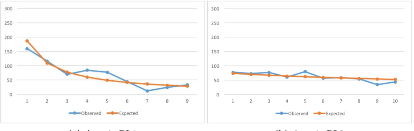
B.1 Austria – Observed Counts vs BL Expected Counts.. . . 52
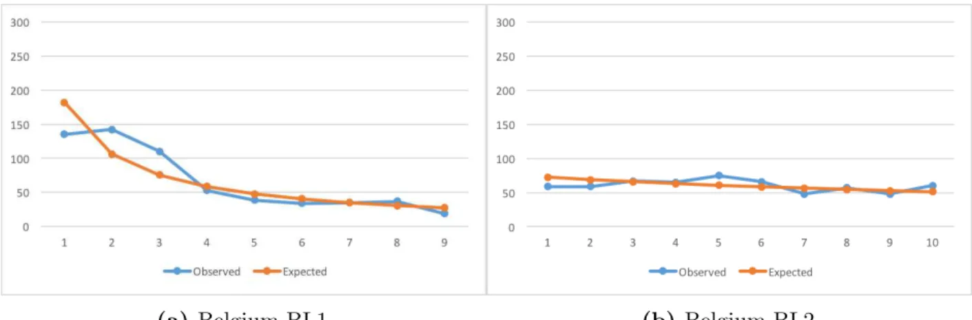
B.2 Belgium – Observed Counts vs BL Expected Counts. . . 53
B.3 Finland – Observed Counts vs BL Expected Counts. . . 53
B.4 France – Observed Counts vs BL Expected Counts. . . 53
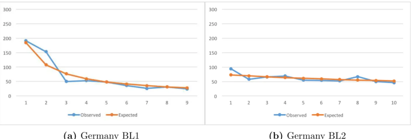
B.5 Germany – Observed Counts vs BL Expected Counts. . . 54
B.6 Greece – Observed Counts vs BL Expected Counts. . . 54
B.7 Ireland – Observed Counts vs BL Expected Counts. . . 54
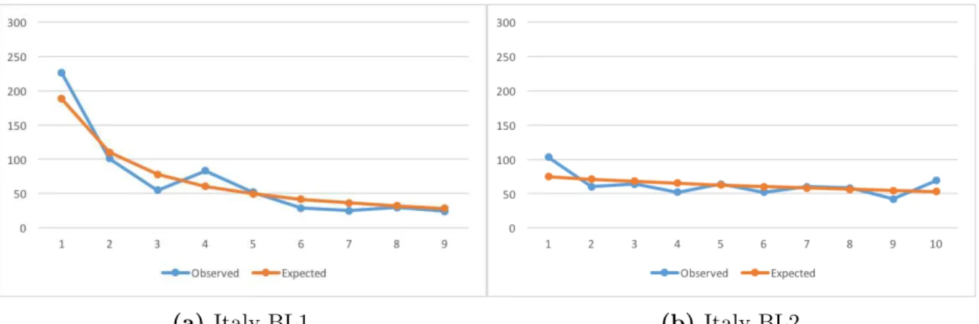
B.8 Italy – Observed Counts vs BL Expected Counts. . . 55
B.9 Luxembourg – Observed Counts vs BL Expected Counts. . . 55
B.10 Netherlands – Observed Counts vs BL Expected Counts. . . 55
B.11 Portugal – Observed Counts vs BL Expected Counts. . . 56
B.12 Spain – Observed Counts vs BL Expected Counts. . . 56
List of Tables
2.1 Benford’s Law Probabilities-First Digit . . . 5
2.2 Benford’s Law Probabilities-Second Digit . . . 6
C.1 Bayes Factor Interpretation Scale . . . 57
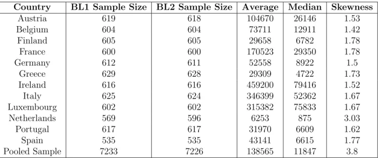
C.2 Datasets and Descriptive Statistics . . . 58
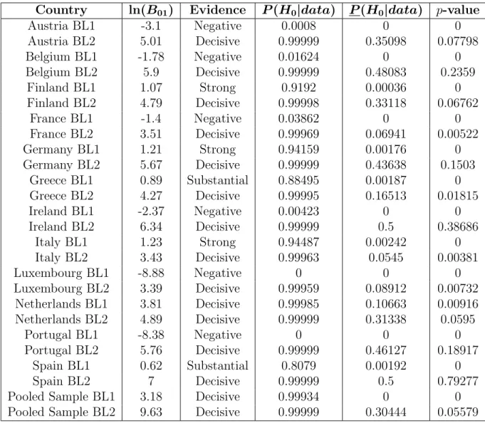
C.3 Chi-Square Goodness-of-Fit and and Multinomial ∧ Dirichlet Model Results – Dirichlet (α=1) Prior . . . 59
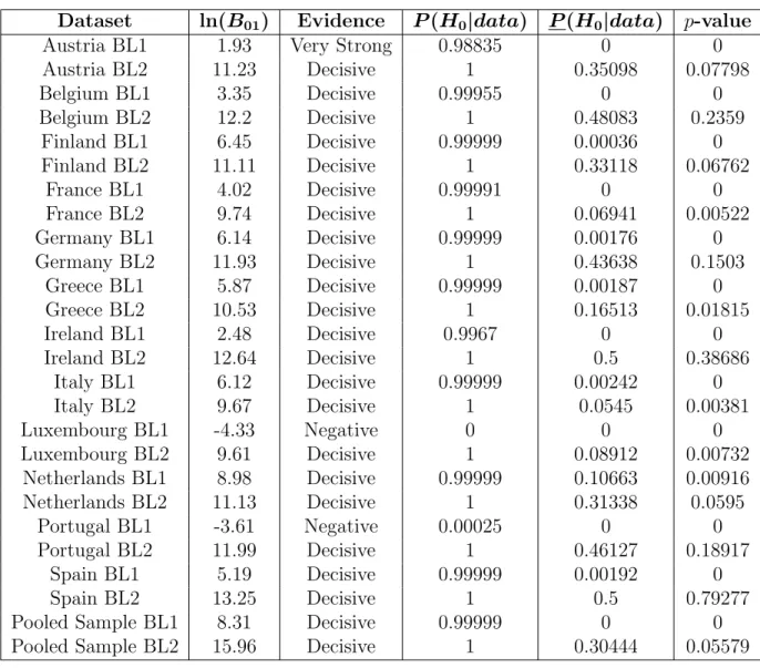
C.4 Chi-Square Goodness-of-Fit and Multinomial ∧ Dirichlet Model Results – Dirichlet (α=θ0) Prior . . . 60
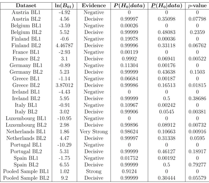
C.5 Chi-Square Goodness-of-Fit and Multinomial ∧ Dirichlet Model Results – Dirichlet (α= 22θ0) Prior and Dirichlet (α= 12θ0) Prior . . . 61
C.6 Austria BL1 – Z-Test and Binomial ∧ Beta Model Results – Beta (1,1) Prior . 62 C.7 Ireland BL1 – Z-Test and Binomial ∧ Beta Model Results – Beta (1,1) Prior . 62 C.8 Luxembourg BL1 – Z-Test and Binomial ∧ Beta Model Results – Beta (1,1) Prior . . . 62
C.9 Portugal BL1 – Z-Test and Binomial ∧ Beta Model Results – Beta (1,1) Prior 63 C.10 Austria BL1 – Z-Test and Binomial ∧Beta Model Results – Beta (22θ0,22− 22θ0) Prior . . . 63
C.11 Ireland BL1 – Z-test and Binomial∧Beta Model Results – Beta (22θ0,22−22θ0) Prior . . . 63
C.13 Portugal BL1 – Z-Test and Binomial∧ Beta Model Results – Beta (22θ0,22−
22θ0) Prior . . . 64
C.14 Variances and Standard Deviations – Multinomial∧Dirichlet Model – Dirichlet (α=1) Prior . . . 65
C.15 Variances and Standard Deviations – Multinomial∧Dirichlet Model – Dirichlet (α=θ0) Prior . . . 65
C.16 Variances and Standard Deviations – Multinomial∧Dirichlet Model – Dirichlet (α=22θ0) Prior . . . 66
C.17 Variances and Standard Deviations – Binomial∧ Beta Model – Beta (1,1) Prior 66
C.18 Variances and Standard Deviations – Binomial∧Beta Model – Beta (22θ0,22−
Acronyms
BF Bayes Factor.
BL Benford’s Law.
BL1 Benford’s Law for First Digits.
BL2 Benford’s Law for Second Digits.
BLDA Benford’s Law based Digit Analysis.
BMS Bayesian Model Selection.
CHT Classical Hypothesis Testing.
CME Conditional Measures of Evidence.
DA Digit Analysis.
DGP Data Generating Process.
LTP Law of Total Probability.
PDF Probability Density Function.
PMF Probability Mass Function.
PP Posterior Probability.
SGPC Stability and Growth Pact Criteria.
Chapter 1
Introduction
“The difficulty lies, not in the new ideas, but in escaping from the old ones,
which ramify, for those brought up as
most of us have been, into every corner
of our minds.”
John Maynard Keynes (1937)
1.1
Motivation and Goals
Contrary to what one might intuitively think, the observed frequencies of leading digits in
numbers from many naturally occurring collections of numbers are not uniform. Instead,
smaller numbers are more likely to occur as first digits than larger numbers. In many such
datasets, about 30% of the entries start with a 1, 18% start with a 2, and so on up to the
less likely leading digit (9), occurring only about 5% of the time. Those are the frequencies
postulated by Benford’s Law (BL).
Digit Analysis (DA) consists in using empirical regularities regarding the occurrence
of digits in numbers, such as BL, to screen numerical datasets for anomalies like erroneous or
fraudulent data. It relies on goodness-of-fit tests, where a point null hypothesis represents
conformance to the expected law. The classical paradigm of hypothesis testing [Classical
proxy to normal behaviour, but because models are supposed to be approximations of the
reality and one can not realistically expect the data to perfectly fit the postulated models
(even when they are true) in all samples, Benford’s Law based Digit Analysis (BLDA) is a
problem where economic and practical significance of the deviation from the expected law is
more important than its statistical significance. Therefore, CHT with fixed dimension, which
according to Pericchi and Torres (2011) over-reject the null hypothesis in large samples due to the high power they attain, making statistical significance prevail over economic significance
may be inappropriate for DA. Wasserstein and Lazar (2016) note that if a sample is big enough then CHT can identify any deviation from the hypothesised law, no matter how tiny,
as statistically significant. BLDA is then likely to produce many false positives, as it identifies
very small deviations from BL, without practical importance, as statistically significant.
One goal of this dissertation is to propose an alternative BLDA methodology, based
on Bayesian Model Selection (BMS). Two model selection environments are presented, one
where conformance to BL frequencies is assessed jointly and is meant to be an alternative to
the classical joint goodness-of-fit tests used in DA, such as the chi-square test, and another
one where agreement to each BL postulated frequency is assessed individually, and is meant
to be an alternative to the classical z-test. Conditional Measures of Evidence (CME) [Bayes
Factors (BFs) and posterior probabilities (PPs)] will be used to quantify the evidence if favour
of the null hypothesis (conformance to BL), instead of the classical and widely used p-value,
which besides being more easily misinterpreted is difficult to perceive in a probability scale
and quantify as the strength of the evidence provided by the data against the null hypothesis.
The other goal is to explore the conflict between CHT and BMS in precise null
hypothesis testing, and its impact to BLDA. Delampady and Berger (1987, 1990) show that CME often support precise hypotheses with tiny p-values, and that even lower bounds on
CME over wide classes of prior distributions often provide more support to the null hypothesis
than the p-value, suggesting that CHT frequently underestimate the evidence provided by
1.2
Structure
This dissertation begins with a brief literature review of the relevant topics, where preliminary
concepts are introduced (chapter 2): first, BL is defined and its empirical evidence is reviewed (section 2.1), then DA is introduced, with particular focus on BLDA (section2.5), section 2.6
addresses the conflict between the two main paradigms of hypothesis testing (the Classical and
the Bayesian) and section 2.7 details the motivation for the choice of the Bayesian approach in the particular problem being addressed. Chapter 3 details the theoretical foundations of the methodology that will be applied: the BFs are derived in sections 3.2 and 3.3, prior distribution specification is discussed in section 3.4, PPs calculation is discussed in section3.5
and the lower bounds on BFs and PPs are addressed in section 3.6. Chapter 4 presents an empirical application of the methodology suggested in chapter 3 using real life data: the data is described in section 4.2, the study design in section 4.3, the study results are presented in 4.4and discussed in section 4.5. The conclusions and the limitations of the approach are presented chapter 5.
1.3
Notation and Terminology
A number’s first digit, which may also be referred to as that number’s most significant digit,
leading digit or mantissa, is the first element of the number’s floating point representation and
will be denotedD1. Likewise, Dkrepresents the kth most significant digit in a number: thekth
entry of the number’s floating point representation. The base 10 logarithm ofxwill be denoted
log(x), and its natural logarithm as ln(x). The CME should be interpreted as measures of
evidence conditioned by the data, not the ones conditioned by the truth of the null hypothesis:
this includes BFs and PPs and excludes p-values. All BFs in this work are BFs in favour
of the null hypothesis. Bold Greek letters represent vectors, capital Greek letters represent
parameter spaces and lower case Greek or Latin letters represent parameters. In situations
of no ambiguity, the null hypothesis may be referred to as just “the null”, the alternative
hypothesis as “the alternative” and the prior distribution as “the prior”. The Bayesian model
combining the prior distribution h(θ) with the likelihood f(x|θ) will be textually denoted as
Chapter 2
Literature Review
“The law of probability of the occurrence of numbers is such that all mantissae of
their logarithms are equally probable.” Simon Newcomb (1881)
2.1
Benford’s Law: History and Definition
BL is due to Simon Newcomb and Frank Benford. Newcomb (1881) noticed that books logarithmic tables were more worn out on the first pages and progressively cleaner throughout,
suggesting that the larger a number’s starting digit the less looked up to that number was.
Based on this observation, he made the conjecture on the epigraph of this chapter, which
implies the logarithmic relation in equation 2.1 (BL) and the probabilities in table 2.1. Benford (1938), through a dataset of 20229 observations from 20 different variables, showed that Newcomb’s conjecture did fit many real life collections of numbers.∗
P(D1 =d1) = log(d1+ 1)−log(d1) = log
1 + 1 d1
, d1 ∈ {1, . . . ,9} (2.1)
Benford’s (1938) study consisted in collections of numbers from such diverse sources as river surface areas, population sizes, physical constants, numbers in newspapers front pages, all the
∗ Diaconis and Freedman (1979) provided convincing evidence that Benford manipulated round-off errors
d1
dd11 1 2 3 4 5 6 7 8 9
P(D1 =d1) 0.3031 0.1761 0.1249 0.0969 0.0792 0.0669 0.0580 0.0512 0.0459
Table 2.1: Benford’s Law for First Digits (BL1) probabilities
numbers inside a Reader’s Digest issue, the heat of chemical compounds, molecules weight,
drainage rates, death rates, atomic weights, baseball statistics, addresses from the first 342
people listed on the American Men of Science, sequences of powers, factorials and square
roots, among others.
Through equation 2.1 and table 2.1 it is easy to see that, according to BL, the distribution of leading digits in numbers is far from uniform. Instead, it shows a logarithmic
decay. Because DA often uses frequencies of digits other than the first, it is necessary to
generalize BL for digits beyond the first (equations 2.4 and 2.5), as well as for combinations of digits (equations 2.2 and 2.3)∗:
P(D1 =d1, D2 =d2) = log
1 + 1
10d1+d2
(2.2)
P(D1 =d1, . . . , Dn =dn) = log
1 + n 1
P
i=1
10n−id i (2.3)
P(D2 =d2) = 9
X
d1=1
log
1 + 1
10d1 +d2
(2.4)
P(Dn =dn) =
9
X
d1=1
10
X
d2=0 · · ·
10
X
dn−1=0
log
1 + n 1
P
i=1
10n−id i (2.5)
wheredi ∈ {0,1, . . . ,9}for digits beyond the first. Equation 2.2 is the joint Probability Mass
Function (PMF) of D1 and D2, the first two digits, and equation 2.3 is the joint PMF of D1, . . . , Dn, the first n digits. The marginal PMF of D2 (equation 2.4) is obtained by using the lLaw of Total Probability (LTP) on equation 2.2to sum across all possible values of d1, and the marginal PMF of the nth most significant digit (equation 2.5) is obtained by using
the LTP on equation 2.3. Benford’s Law for Second Digits (BL2) probabilities, resulting from equation 2.4, can be consulted in table 2.2. There is still a decreasing pattern, although less
d2
dd22 0 1 2 3 4 5 6 7 8 9
P(D2 =d2) 0.1197 0.1139 0.1088 0.1043 0.1003 0.0967 0.0934 0.0904 0.0876 0.0850
Table 2.2: Benford’s Law probabilities for the second digit.
evident. For the third digit the probability is nearly uniform and for the forth and following
the deviation from uniformity is inappreciable [see Berger and Hill (2015, p.2)]. Diaconis (1977) demonstrated that as n gets larger the distribution of Dn converges in exponential
time to uniformity.
2.2
Benford’s Law: Empirical Evidence
Subsequent to Benford’s (1938) work, an abundance of additional empirical evidence has been found in many different domains, such as physics, biology, demographics, and computer
science. Some examples of conformance to BL that can be found in the scientific literature
are: lists of physical constants [Knuth (1981), Burke and Kincanon (1991)]∗, decimal parts of failure (hazard) rates (Becker, 1982), radioactive half-lives [both measured and calculated (Buck, Merchant, and Perez, 1993)], long series of floating point numbers from scientific calculations [Knuth (1981), Hamming (1970)], sequences of factorials (Sarkar, 1973), powers of integers†, Fibonacci numbers (Washington, 1981) and Lucas numbers (Giles, 2007), repeated calculations with real numbers (Knuth,1981), powers of random numbers (or their reciprocals) as the exponent gets larger, products of random numbers as the number of terms in the
product gets higher‡ (Adhikari and Sarkar, 1968), prime numbers in large finite intervals (Luque and Lacasa, 2009)§, the distribution of cells per colony in certain cyanobacterium (Costas et al., 2008), basic genome data (Friar, Goldman, and P´erez–Mercader, 2012), daily pollen counts in European cities (Docampo et al., 2009), population sizes [Nigrini and Wood
∗ Jamain (2001) warned to the fact that these results regarding physical constants may not be very
convincing as the samples are usually not large enough to allow strong statistical conclusions.
† See Raimi (1976) for the powers of two. A generalization for powers of higher order is a consequence of
the equidistribution theorem.
‡ Schatte (1988) extended this idea for sufficiently long computations in floating-point arithmetic. § Although for this case it is a generalized version of the Benford’s law [see Pietronero, Tosatti, Tosatti,
(1995), Jamain (2001), Hill (1995-b)], numbers (Varian, 1972) and regression coefficients (T¨odter, 2009) in scientific publications, vote counts in electoral processes [Torres (2006), Pericchi and Torres (2011)] and the set of all numbers on the World Wide Web (Berger and Hill, 2015, p. 4-6). More important for the purpose of this dissertation are the findings in the fields of economics, finance and accounting: gross domestic product growth rates (Nye and
Moul, 2007), many macroeconomic time series such as banking statistics, national financial statistics and balance of payment statistics (Gonzalez-Garcia and Pastor, 2009), business invoices and financial forecasts (Varian, 1972), most of the accounting data [Nigrini (1992,
1995 1999,1997, 2012)]∗, reported income tax data (Nigrini,1996), interest received in United States (US) tax returns (Berger and Hill, 2015), 1-day returns on the Dow-Jones Industrial Average Index and on the Standard and Poor’s Index for stock prices (Ley, 1996), the main Chinese stock market indices (Shengmin and Wenchao, 2010), and the Madrid, Vienna and Zurich stock market prices (Pietronero et al., 2001).
2.3
Benford’s Law: Invariance
†Other distinctive properties of BL conforming datasets is that their leading digit distributions
are scale invariant (Pinkham,1961), base-invariant (Hill,1995-a), inversion invariant‡(Benford,
1938) and sum invariant (Allaart, 1997). This means that if one begins with a BL conforming dataset and either multiply all entries by a constant, divide one by each entry, or convert all
entries to another base§, the observed frequencies of leading digits will remain approximately
constant. For other invariances of BL see Jamain (2001). It is demonstrated that BL is the only possible leading digit distribution with such properties, that is, if the frequencies
of leading digits in a numerical dataset are either scale invariant (Pinkham, 1961)¶, base
∗ Nigrini found that lists of items such as accounts receivable or payable, transactions, inventory accounts,
fixed asset acquisitions, daily sales, refunds and disbursements all follow BL.
† For a comprehensive and rigorous review of BL invariance properties see Berger and Hill (2011). ‡ Some tabulations of data are given in reciprocal form, such as candles per watt and watts per candle, as
Benford (1938) exemplified. If one form of the tabulation follows BL then its reciprocal also does.
§ When converting numbers to another base, the set of possible first digits will differ. Therefore, the leading
digits frequencies can not remain the same. However, changing the base will preserve the logarithmic decay in frequencies if the original dataset follows BL (Smith,2002). The generalization of BL1 for base bisfD1(d1) = logb(1 + d11), ford1 from 1 up tob−1 (Hill,1995-b).
¶ Knuth (1981) and Hill (1995-a) accused Pinkham (1961) of making unwarranted assumptions about the
invariant (Hill, 1995-a) or sum invariant (Allaart, 1997) then BL must hold.
2.4
Where can the Benford’s Law be Found?
There has been a lot of attempts at explaining the emergence of BL [see Raimi (1976), Hill (1995-b), Scott and Fasli (2001), Jamain (2001), Smith (2002), Fewster (2009), Nigrini (2012) or Berger and Hill (2015) for reviews]. It is accepted that the first rigorous explanation was due to Hill (1995-b), who demonstrated that if random samples from different randomly-selected (in any unbiased way) probability distributions are combined, then the leading digit frequencies
in the pooled sample converge to BL. This result helps explaining why BL arises so often.
While numbers describing some phenomena are under the control of a single distribution
(for example: the height of adult men behave according to a normal distribution), many
others are dictated by a random mix of all kinds of distributions. A good example is the
dataset resulting from pooling together all the numerical values in a firm’s financial statement:
the numbers will respect to many different variables, each behaving according to it’s own
Data Generating Process (DGP). The same principle applies for the set of all numbers in
a Census form, tax report, scientific article or magazine. This is congruent with Benford’s
(1938) findings: he used numbers from 20 different domains, and the pooled sample fitted BL very well, even if some of the datasets did not when considered separately.
Some rules of thumb can help assessing whether a dataset should be expected to
conform to BL. The dataset’s mean should be larger than its median and the data’s histogram
should be positively skewed (Wallace, 2002). The graphical representation of the data should resemble a geometric sequence (without artificial truncation) and the logarithm of the
difference between the largest and smallest values should be close to an integer value (Nigrini,
2012). The larger the ratio of the mean divided by the median, the most likely the fit is (Durtschi, Hillison, and Pacini, 2004). The numbers should represent quantities, amounts or sizes, should be free of imposed limits∗ (bounded sequences with restricted significant digits
actually not so rare. Quoting Jones (2002): “In the search for order and laws in complex systems there has been the realisation that much of life is scale invariant.”.
∗ The “free of imposed limits” assumption may be relaxed as long as the data spans two orders of magnitude
like hours of the day, months or years, human age or weight and the set of all integers are
not good fits), should not be assigned sequentially (like phone numbers, checks and lottery
numbers), and should not be influenced by human thought (ATM withdrawals, donations,
prices or values set at psychological thresholds such as rounded quantities). Datasets where
each entry consists in the arithmetical combination of multiple numbers, are also very likely
to behave according to BL.∗. Scott and Fasli (2001) consider that the best candidate datasets to reproduce BL are the ones with only positive values, uni-modal (and non zero mode)
positively skewed distribution in which the median is no more than half of the mean. This
implies a lognormal distribution with scale parameter larger than 1.2 for the data.†
Considering the discussion above, most economical and financial datasets are obvious
candidates to fit BL: They consist in the aggregation of observations from several different
variables (such as the set of all numbers in a firm’s financial statement or in a government’s
budget report) and their entries consist in quantities or amounts that can be interpreted (and
are generated) as the mathematical combination of several other variates‡.
2.5
Benford’s Law and Digit Analysis
DA consists in using empirical regularities regarding the occurrence of significant digits in
numbers to detect erroneous or fraudulent data. The idea is to model a baseline frequencies
∗ Recall the already mentioned findings of Adhikari and Sarkar (1968) about products of random numbers,
Hamming (1970) and Knuth (1981) about long series of floating point numbers from scientific calculations, Sarkar (1973) about factorials, Raimi (1976) about powers of integers, Knuth (1981) about repeated calculations with real numbers and Schatte (1988) about long computations in floating point arithmetic. Also, Raimi (1969) and Boyle (1994) argue that multiplying random numbers produces conformance to BL and Boyle (1994) showed that BL is the limiting distribution of leading digits when random variates are repeatedly multiplied, divided or raised to integer powers. Scott and Fasli (2001) showed that when each number in a dataset is a product of many terms, the first digit distribution converges to BL as the number of terms in the product increases. This holds for products of random variates, successive multiplication by a new realization of the same random variable and for successive multiplication by a constant. For products with fewer terms it is possible that full convergence is not reached but a monotonic decay in the frequencies is still likely to be present.
† The “only positive values” condition is not as restrictive as it may look. Note that taking the absolute
value of all entries in a dataset leaves the leading digit distribution unchanged.
‡ Trivial example: Revenue=price×quantity. Every variable that can be modelled by an equation, can be
distribution representing normal behaviour and then attempt to detect if some particular
dataset significantly departs from it (Bolton and Hand,2002). According to Durtschi, Hillison, and Pacini (2004) various forms of DA have long been used by auditors when performing analytical procedures, such as checking transaction records for duplicate payments. BL, when
applied to detect fraudulent or erroneous data, is just a more complex form of DA. BLDA is
only applicable to usually BL conforming datasets, and as seen in section 2.4, this includes most of the economic and financial data.
Varian (1972) was the first to suggest the application of BL to DA. The idea is that in datasets of naturally generated numbers (i.e. without intervention) where digit frequencies
conform BL, replacing numbers with fabricated ones typically results in deviation from BL.
As discussed in section2.4, numbers influenced by human thought usually do not conform BL, and hence manipulating numbers from a BL conforming DGP leaves a detectable trace
in the data. This may happen for many reasons, like the fact that numbers influenced by
human thought are usually tied to psychological thresholds. Durtschi, Hillison, and Pacini
(2004) note that someone creating false numbers usually (and subconsciously) favours certain numbers, and may also be biased against certain numbers in an attempt to conceal their
actions. Nigrini and Mittermaier (1997) note that when entering fraudulent data, people tend to use the same (or similar) amounts often, moving the observed digit frequencies away from
BL. Also, fraudsters are usually unaware of the properties of the DGP behind the data they
are manipulating, and consequently tend to distribute the made-up entries leading digits more
uniformly than a BL law conforming DGP would. Cho and Gaines (2007) find it very unlikely that someone manipulating numbers would seek to preserve conformance to BL, because even
though it is widely applicable it is not widely known. Moreover, experimental research has
shown that people do a poor job in replicating random data even when they are told what the
DGP is (Camerer, 2003, pp. 134-138). Bolton and Hand (2002) consider the premise behind fraud detection using tools such as BL to be the fact that fabricating data which conforms to
BL law is difficult. Diekmann and Jann (2010) consider that in order to ascertain the validity of a BLDA it is necessary to demonstrate that the true data is in accordance to BL and the
A wide literature exists on the application of BLDA. Carslaw (1988) analysed New Zealand firm’s earnings and found that the numbers contained more zeros in the second digit
than expected according to BL, suggesting that firms were manipulating (rounding up) their
earnings. Thomas (1989) studied US firms earnings and found that firms reporting losses exhibit the reverse pattern (rounded down numbers), and also found evidence of manipulation
(through rounding of numbers) in earnings per share data. Other studies where BL is used in
the detection of earnings manipulation are: Niskanen and Keloharju (2000), Kinnunen and Koskela (2003), Caneghem (2002,2004), Skousen, Guan, and Wetzel (2004), Nigrini (2005) and Guan, He, and Yang (2006). Nigrini (1992,1996) was the first to extensively apply BL to accounting data with the goal of detecting fraud. He also used it to help identifying tax
evaders, and so did Watrin, Struffert, and Ullmann (2008) and M¨oller (2009). Diekmann (2007) applied BL to scientific fraud detection∗, and Asllani and Naco (2014) used it to screen hospital spendings for numerical anomalies. Nye and Moul (2007), Gonzalez-Garcia and Pastor (2009), Judge and Schechter (2009), T¨odter (2009), Rauch, G¨ottsche, Br¨ahler, and Engel (2011) used BL to assess the quality of economic data and macroeconomic statistics. Marchi and Hamilton (2006) found evidence of manipulation in self-reported regulatory data in the Toxic Release Inventory: while reported emissions of some chemicals did not fit BL, the
measured values of the same chemicals did. They concluded that manipulation in the data
may be the reason why large drops in air emissions reported by firms are not always matched
by similar reductions in measured concentrations by pollution monitors. Giles (2007) studied a dataset of winning bids from eBay auctions and because the numbers fitted BL he found
no evidence of collusion among bidders nor shill among sellers. Prudˆencio (2015) analysed the financial statements of three Portuguese commercial banks from 2007 to 2013 and found
significant deviations from BL. One of those banks, Banco Esp´ırito Santo, went Bankrupt in
2014 and its former president, board of directors and other high level employees are facing
several charges including manipulation of accounting numbers. Haynes (2012) analysed financial statements from bankrupt municipal governments and found overall nonconformity
to BL. He concluded that such screening, had it been done earlier, could have identified that
∗ Recall the findings of Varian (1972) and T¨odter (2009) mentioned in section2.2: regression coefficients
something was amiss. DA is also being used to screen and validate numbers from electoral
processes [Mebane (2006-a, 2006-b, 2007), Torres (2006), Pericchi and Torres (2004,2011), and Torres, Fernandez, Gamero, and Sola (2007)].
2.6
Paradigms of Hypothesis Testing
In the classical approach to hypothesis testing [Fisher (1925), Neyman and Pearson (1933)], a significant finding is declared when the value of a test statistic exceeds a specified threshold,
with values of the test statistic above that threshold defining the rejection region. The
significance level (also known as dimension) of the test is defined as the maximum probability
that the test statistic falls into the rejection region when the null is true. Fisher (1925) proposed the p-value (the probability, conditioned on the null hypothesis being true, of obtaining a test
statistic which is at least as unlikely as the one actually observed) as a measure of discrepancy
between observed data and null hypothesis. For its simplicity and apparent objectivity, the
p-value became the standard of measure evidence against an hypothesis (Schervish, 1996). In the Bayesian approach, initially developed by Jeffreys (1935, 1967), statistical models represent the DGP of the data under each of two competing hypotheses, the BF
compares the predictive density of the observed data under one model with that of the
alternative model, and the Bayes (1763) theorem is used to compute the PP of the hypotheses. As Kass and Raftery (1995) note, Bayes theorem updates prior probabilities into PPs through consideration of the data. The update represents the evidence provided by the
data, and it is the same regardless of the prior probabilities. In the odds scale, the update
corresponds to the BF, and represents the relative predictive density of the data under one
of the hypotheses compared with that of the alternative. The BF is a measure of change in
support, as it measures the change in prior odds in favour of one hypothesis after the data is
observed (Lavine and Schervish, 1999). Bernardo and Smith (1994) intuitively describe the BF as a measure of whether (and by how much) the data have increased or decreased the
odds in favour of one of the hypothesis. Unlike thep-value, BFs depend only on the predictive
hypotheses being compared form a partition of the parameter space, with the alternative
corresponding to the bilateral composite hypothesis of divergence from a point null which
represents conformance to BL, the specification of the alternative is automatic, and therefore
one of the main critiques to this approach [the subjectivity involved in the specification of
the alternative when there is no objective choice (Johnson, 2013)] does not apply. However, the specification of a prior distribution for the alternative is unavoidable. This drawback can
be mitigated by finding lower bounds on the CME over wide classes of prior distributions.
These two paradigms of hypothesis testing often produce seemingly incompatible
results. Edwards, Lindman, and Savage (1963), Berger and Delampady (1987,1990), Berger and Sellke (1987), and Lin and Yin (2015) show that evidence against the null hypothesis provided by CME can differ by an order of magnitude from the p-value, when testing a
precise null hypotheses, raising concerns about the routine use of moderately small p-values
and significance levels. A p-value of 0.05, conventionally labelled as a significant result and
considered strong evidence against the null in the classical approach, can result in a PP of at
least 0.3 in favour of the null hypothesis∗. To solve this, Johnson (2013) considers that, in CHT, evidence thresholds should be decreased to 0.005 for the declaration of a significant
finding and to 0.001 for a highly significant finding†. This contradicts Fisher (1925), for whom a p-value below 0.05 was a safe indicator of a significant result, but agrees with Taleb
(2016), who warns that due the skewness and volatility of a p-value’s meta-distribution (across repetitions of the same experience), to get what people mean by 5% confidence level, ap-value
almost one order of magnitude smaller than conventional is needed.
The apparent discrepancy between the two paradigms is due to the fact that they rely
on the calculation of different probabilities. p-values and significance levels are conditioned on
the null hypothesis being true, and so they can not be a direct measure of the probability of
that hypothesis (Goodman, 1999-b). PPs represent actual the probability of the hypotheses being true conditioned on the observed data, which is more straightforward to interpret,
∗ To highlight the conflict between thep-value and the CME, Berger and Delampady (1987, 1990) and
Berger and Sellke (1987) showed that, in precise hypothesis testing, even the lower bounds on BFs and PPs that are found over wide classes of prior distributions are often much larger than the corresponding p-values. Therefore, one can not dismiss this conflict by arguing that the discrepancies are due to the specific prior distribution that was chosen.
† In terms of BFs, Johnson’s (2013) revised standards for statistical evidence correspond to values from 25
as it is more natural to think in terms of the probability of an hypothesis given the data
than in terms of the probability of the data given that the hypothesis is true. Still, a lot
of practitioners incorrectly interpret a p-value of 0.05 as the null hypothesis having a 5%
probability of being true, or as a 5% error rate on the rejection of the null, misinterpretations
which Goodman (1999-a) popularized as “thep-value fallacy”∗.
2.7
Why the Bayesian Approach?
Conformance to BL is a goodness-of-fit problem and hence BLDA relies on goodness-of-fit
statistical tests. Large samples are always preferable, to give the DGPs a chance to reveal its
true properties. Unfortunately, according to Pericchi and Torres (2011), the usefulness and interpretation of the p-value on classical test statistics is drastically affected by sample size,
and Goodman (1999-a), Wasserstein and Lazar (2016) warn that the p-value and statistical significance do not take into account the size of the observed deviation from the null: any
deviation, no matter how small, can produce a smallp-value if the sample size or measurement
precision is high enough. Consequently, very small deviations from the null, with no practical
importance, are likely to be considered statistically significant†. Conversely, large deviations
can produce large p-values if the sample is small or if the measurements are imprecise, similar
deviations can have different p-values for different sample sizes and similar p-values may
correspond to different deviations in different samples.
Despite thep-value being able to indicate how incompatible the data is with a specified
hypothesis (Sellke, Bayarri, and Berger, 2001), knowing the data to be rare under one hypothesis is of little use unless one determines how rare it is under the alternative hypotheses.
Hence, although in classical hypothesis testing the smaller the p-value, the more significant
the deviation from the null is, it is difficult to perceive the p-value in a probability scale and
quantify it as the strength of the evidence in the data against the null, as the p-value only
provides one side of the information [Lin and Yin (2015), Wasserstein and Lazar (2016)]‡.
∗ Other references on the susceptibility of thep-value to be misinterpreted are: Gibbons and Pratt (1975),
Schervish (1996), Matthews (1998), O’Hagan and Luce (2003) and Hubbard and Bayarri (2003).
† As Wasserstein and Lazar (2016) note, statistical significance is not equivalent to scientific, human, or
economic significance.
The practice of summarizing results into either statistically significant or non-significant
and drawing a sharp distinction between them, standard in classical hypothesis testing, can
also be misleading: besides encouraging the dismissal of potentially important evidence
in favour of null, any particular threshold separating significance from non-significance is
arbitrary∗, and even large changes in observed significance levels can correspond to small,
non-statistically nor practically significant changes in the underlying test statistics (Gelman
and Stern, 2006). Wasserstein and Lazar (2016) consider this dichotomy to distort the scientific process and warn that scientific conclusions and business or policy decisions should
not be based only on whether a p-value passes a specific threshold.
In BLDA, economic and practical significance of the deviation from BL is more
important than it’s statistical significance, as one cannot realistically expect the observed
data to perfectly conform BL in all samples, even when BL hypothesis is true. Therefore,
CHT with fixed dimension, in which statistical significance is known to overweight economic
significance and which according to Pericchi and Torres (2011) are known to over-reject the null hypothesis (which in this case represents conformance to BL) in large samples, may not
be adequate, as they are likely to produce many false positive results. According to Ley
(1996), the over-rejecting nature of such tests is due to the huge power they attain in large samples, with the acceptance region shrinking with sample size, for a given significance level.
Leamer (1983) considers this to be a weakness of the classical method, as models are to be considered mere approximations to reality instead of perfect DGPs.
Aware of all this, Ley (1996) addressed BLDA in a Bayesian way. Despite his posterior distribution based parameter estimates being very close to BL theoretical ones, the classical
likelihood-ratio and chi-square tests would reject BL hypothesis in all datasets†. Torres (2006) and Pericchi and Torres (2011) used the Jeffreys model selection approach, based on BFs, PPs and respective lower bounds, and concluded that datasets with apparently very good fit
to BL could have nearly zero p-values.
resulted in a miscarriage of justice is the Sally Clark trial. See Green (2002) or Bram (2014, p.55)
∗ Only a very small change in some test statistic is required to move from a observed significance level of
0.51 (non-significant) to 0.49 (significant). According to Matthews (1998), even Fisher when asked why his figure of 0.05 was a safe threshold at which to declare a result as significant, admitted he did not know at all, and that he simply chose 0.05 because it was convenient.
† The same hypothesis was not rejected in the smaller samples resulting from considering only the last
Chapter 3
Bayesian Digit Analysis: Theoretical
Framework
“If we have no information relevant to the actual value of the parameter, the
(prior) probability must be chosen so as
to express the fact that we have none.” Harold Jeffreys (1967)
3.1
Introduction
In a collection of N nonzero numbers there areN first digits, assumed to have been generated
according to some 9-variate multinomial density f(x|θ), and M second digits (M ≤ N)
assumed to have been generated according to some 10-variate multinomial density f(y|ξ).
Because this dissertation focus in BL1 and BL2 based DA, what we want is to check whether
or not, in a given sample, θ and ξ (the parameter vectors from the multinomial DGPs
responsible for the occurrence of first and second digits) are as postulated by BL (tables 2.1
and 2.2, respectively).
Section 3.2introduces the Multinomial ∧Dirichlet model, a Bayesian alternative to the classical joint goodness-of-fit statistical tests commonly used in BLDA.∗ Because joint
goodness-of-fit tests evaluate conformance to BL frequencies as a whole but do not identify
which frequencies are in agreement to BL in a given sample and which are not, Nigrini (2000) incorporated the z-test in DA, which applies individually to each frequency. Section 3.3
introduces the Binomial ∧Beta model, a univariate version of the Multinomial ∧ Dirichlet
model, as an alternative to the z-test in DA.
3.2
Bayes Factor: Multinomial
∧
Dirichlet Model
Consider the random vectors X = (X1, . . . , Xk) and θ = (θ1, . . . , θk), respectively defined
in the subspaces χ = {(x1, . . . , xk) : xi ∈ IN0,Pik=1xi ≤ N} and Θ = {(θ1, . . . , θk) : θi ∈
(0,1),Pk
i=1θi <1}, whereN is the fixed sample size and Θ is the k-dimensional simplex, Sk.
Let X follow a k-category multinomial distribution with unknown parameter vector θ ∈Θ:
X|θ ∼ Mk(N,θ):
f(x|θ) = QkN+1!
i=1 xi! k+1
Y
i=1
θixi (3.1)
with x∈χ, xk+1 =N −Pki=1xi and θk+1 = 1−Pki=1θi.
Let the observed counts of significant digits be represented by x = (x1, . . . , xk)∗, a
realization of X|θ which is assumed to have arisen under one of two possible and mutually
exclusive states of the world (hypothesis/models) relative to θ: H0 with prior probability
P(H0) =π0 orH1 with prior probability P(H1) = 1−π0. Because the null hypothesis usually represents the established theory, in the specific problem being addressed H0 represents
conformity to BL. Let θ0 = (θ01, . . . , θ0k)∈ Θ be the parameter vector of the multinomial
PMF (3.1) underH0. Considering the subspace Θ1 = Θ\{θ0}, the hypotheses being compared
are:
H0 :θ =θ0 vs H1 :θ ∈Θ1 (3.2)
Kolmogorov-Smirnov [see Massey Jr (1951) or Conover and Conover (1999, p.428)] and the Kuiper test (Kuiper,1960), both used with Stephens (1970) correction factor and with Morrow’s (2014) BL specific critical values, the Conover (1972) test, and BL specificm-statistic (Leemis, Schmeiser, and Evans,2000) andd-statistic (Cho and Gaines,2007) to whom Morrow (2014) also computed critical values. For a review of the properties of these tests in BLDA see Morrow (2014).
∗ In BL1 analysisk= 8,x
1represents the count of ones as the first digit,x2represents the count of twos
and so on. In BL2 analysisk= 9,x1represents the count of ones as the second digit,x2 the count of
From Berger and Pericchi (2001), we know that the BF in favour ofH0 is obtained through B01(x) = m0(x)
m1(x), wheremi(x) is the marginal density of the data under Hi:
mi(x) = Z
Θi
f(x|θ)π(θ|Hi)dθ (i= 0,1) (3.3)
where π(θ|Hi) is the prior distribution of θ under Hi, Θi is the parameter space of θ under
Hi andf(x|θ) is the likelihood of θ for a given x. Note that Θ0 =θ0 and as already defined
Θ1 = Θ\ {θ0}. Because H0 is a point null hypothesis,
π(θ|H0) = 1θ0(θ) (3.4)
where 1θ0(θ) is the indicator function ofθin{θ0}. Because the Dirichlet family of distributions
is the conjugate prior of the Multinomial distribution (Turkman and Paulino, 2015), and also because there is a particular distribution in the Dirichlet family that corresponds to the
Berger, Bernardo, and Sun (2015) overall objective prior, a k-variate Dirichelet distribution with parameter vector α= (α1, . . . , αk+1)∈R+k+1 will be assumed for the prior distribution
of θ under H1, i.e. θ|H1 ∼Dirk(α):
π(θ|α, H1) = Γ(
Pk+1
i=1 αi) Qk+1
i=1 Γ(αi) k+1
Y
i=1
θiαi−1dθ (3.5)
where Γ(·) is the Gamma function. This prior is centered on E(θ|α, H1) = α
Pk+1 i=1αi
and is
symmetric if αi =α ∀i. Using 3.1, 3.4 and 3.5 on3.3:∗
m0(x) = QkN+1!
i=1 xi! k+1
Y
i=1
θ0ixi (3.6)
m1(x) = QkN+1!
i=1 xi!
B(α+x)
B(α) (3.7)
whereB(α) =R
Θ1 Qk+1
i=1 θiαi−1dθ andB(α+x) = R
Θ1 Qk+1
i=1 θiαi+xi−1dθ are multivariate Beta
functions. Finally, dividing 3.6 by3.7† B01(x) =
Qk+1
i=1 (θ0ixi)Qki=1+1[Γ(αi)]Γ[Pki=1+1(αi+xi)]
Γ(Pk+1 i=1 αi)
Qk+1
i=1 Γ(αi+xi)
(3.8)
with θ0k+1 = 1−Pki=1θ0i. Besides the digit counts, x1, . . . , xk+1, and the null hypothesis
multinomial probabilities θ01. . . , θ0k+1, this BF depends on the Dirichlet hyperparameters,
α1, . . . , αk+1, whose specification will be discussed in section 3.4.
3.3
Bayes Factor: Binomial
∧
Beta Model
From the X|θ ∼ Mk(N,θ) assumption, it follows that each element in X is Binomially
distributed: Xi ∼ Bin(N, θi)∀i ∈ {1, . . . , k}. When assessing conformance to one of BL
frequencies individually, a sample of N numbers corresponds the realization ofN Bernoulli
trials, where a success is the occurrence of the first digit whose frequency is being assessed.
Consider Y = (Yi, . . . , YN), a vector of N independent Bernoulli random variables,
Yi ∼ Bin(1, θ), for some unknown θ ∈ Θ = (0,1). Then X =
PN
i=1Yi ∼ Bin(N, θ). Let
y = (yi, . . . , yN) be a realization of Y and x= Pni=1yi the corresponding realization of X.
The likelihood of θ for a given xin a sample of fixed size N is:
f(x|θ) =
N x
θx(1−θ)N−x (3.9)
The data,x, is assumed to have arisen under one of two possible and mutually exclusive
hypothesis relative to θ: H0 with prior probability P(H0) = π0 or H1 prior probability
P(H1) = 1−π0. Again, H0 represents conformity to BL. Let θ0 ∈ (0,1) be the parameter of the binomial PMF (3.9) under H0, and define Θ1 = (0,1)\ {θ0}. The hypothesis being compared are:
H0 :θ =θ0 vs H1 :θ∈Θ1 (3.10)
Because the Beta family is the conjugate prior of the binomial distribution (Turkman
and Paulino, 2015), and considering the fact that H0 is a point null hypothesis, the assumed prior distribution for θ is:
π(θ|Hi) =
1θ0(θ) if i= 0 θa
−1(1−θ)b−1
B(a,b) if i= 1
(3.11)
where B(a, b) = Γ(Γ(ab)Γ(+bb)) = R1
0 θ
a−1(1−θ)b−1dθ is the beta function, 1
θ0(θ) is the indicator
function of θ0 in Θ, θ
a
−1(1−θ)b−1
distribution andE(θ|a, b, H1) = a
a+b. The marginal densitiy of the data under each hypotheses
is obtained through a univariate version of 3.3: mi(x) =
Z 1
0
f(x|θ)π(θ|Hi)dθ (i= 0,1) (3.12)
Combining 3.11 with 3.12 and considering the hypothesis in 3.10: m0(x) =
N x
θ0x(1−θ0)N−x (3.13)
m1(x) =
N x
B(x+a, n−x+b)
B(a, b) (3.14)
and finally, dividing 3.13 by3.14, the BF in favor of H0 is:∗ B01(x) = θ0(1−θ0)
N−xΓ(a) Γ(b) Γ(n+a+b)
Γ(a+b) Γ(n+a−x) Γ(x+a) (3.15)
The specification of the hyperparametersa and b will be discussed in the next section.
3.4
Prior Distribution Specification
The criticism that Bayesian methods require subjective prior specification has been effectively
answered by the development of objective Bayesian methods based on non informative priors
(Kass and Wasserman,1996). However, Berger and Delampady (1987) note that such methods are not always available, and that precise null hypothesis testing is an example of a situation
where objective procedures do not exist, because even thought one can avoid prior probabilities
specification by focusing on BFs, there is no prior distribution specification that can claim to
be objective. Nevertheless, there are properties to impose on a prior distribution for it to
be considered adequate. Berger and Delampady (1987, 1990) argue that an adequate prior for precise null hypothesis testing should be uni-modal, symmetric about the null parameter
value or at least centered on it, and non increasing about that same point†, to acknowledge
the central role of the null parameter value (representing the established theory), and avoid
treating parameter values other than that as special.
∗ Derivations of3.13,3.14and3.15in appendixA.2. † i.e. symmetric about (or centered in)θ
0, non increasing aroundθ0for the Multinomial∧Dirichlet Model
In the Multinomial∧Dirichlet Model, if α = 1 is set [like in Pericchi and Torres (2011) and Torres (2006)], 3.5reduces the PDF of a uniform distribution on Sk, which is in
conformance to the Bayes-Laplace principle of indifference: assuming equiprobability of events
in the absence of prior knowledge (Syversveen, 1998). For a uniform prior to be obtained in the Binomial∧Beta Model seta =b = 1. The fact that uniform priors are not invariant to
re-parametrizations (Paulino, Turkman, and Murteira, 2003) is not problematic in DA as we are only concerned about parameters, not functions of them. Uniform priors are symmetric,
and non increasing in all their domain, hence being non increasing around the null parameter
values. For BLDA they are not centered on the null parameter values∗.
Instead, ifα=1 1
k+1
is set in the Multinomial∧Dirichlet Model, 3.5 becomes the PDF of a Dirk
1(k+11
],which is the overall objective prior (Berger, Bernardo, and Sun, 2015) for the multinomial distribution. Equivalently, if a = b = 1
2 is set on the Binomial∧Beta Model, the reference prior for the binomial distribution is obtained (Yang and Berger, 1996), and because the Binomial∧Beta is a single parameter model, the reference prior is equivalent
to the Jeffreys prior, which unlike the uniform prior is invariant to reparametrizations (Yang,
1995). The overall objective prior and the reference prior obtained above are symmetric†, but centered in points other than BL null‡. Moreover, because they are symmetric about their
mean, they also fail being non increasing around the null parameter value (for a=b= 1 2 the Beta distribution is U-shaped and symmetric about 12). Therefore, even though the reference
prior has the appealing conceptual interpretation of materializing a truly non-informative prior
[Bernardo (1979), Berger and Bernardo (1992-a,1992-b), Berger, Bernardo and Sun (2009)] and although both the reference and the overall objective prior have desirable properties for
posterior distribution-based inference (Berger, Bernardo, and Sun, 2015), they are designed for estimation and may not be adequate for this particular BMS problem, as they spread
prior density around parameter values other than the null parameter values.
To center a Dirichlet prior on θ0 is only possible assuming α=cθ0 for some c >0
(Delampady and Berger, 1990). However, ifθ0 is the vector with BL1 or BL2 probabilities
∗ The uniform prior is centered on 1( 1
k+1) in the Multinomial∧Dirichlet Model and on 1
2 in the
Binomial∧Beta Model.
† The Dir
k distribution is symmetric when αi=α∀i∈ {1, . . . , k+ 1}, and the Beta (a,b) whena=b. ‡ Because π(θ) ∼ Dir
k(α) ⇒ E(θ) =
α
Pk+1
i=1αi
, the overall objective prior is centered on 1(k+11 ), and becauseθ∼Beta(a, b)⇒E(θ) = a
a+b the reference prior is centered on
and α=cθ0 is assumed, the resulting Dirichlet prior is not symmetric, as αi 6=αj fori6=j.
Equivalently, to center the Beta prior on θ0, the necessary assumption are a = s θ0 and
b =s(1−θ0) for some s >0, which again results in a asymmetrical prior for the specific case of BL1 and BL2 analysis∗. Hence, to use the BFs in 3.8 or 3.15, we have to give up either on the prior being symmetric or in the prior being centered on the null parameter value. Giving
up on symmetry seems to have a lower cost: although in the absence of prior knowledge it is
desirable to have a symmetric prior, as there is no particular reason to skew the prior density
towards any particular region in the parameter space, in BLDA the null corresponds to a
established theory, so it might be acceptable to skew the prior distribution towards a region
in parameter space suggested by that theory. On the other hand, there is no justification for
the prior density to be centered around a point other than the null parameter value.
Because the Dirichlet parameters affect the dispersion of the prior density and
consequently define how informative the prior distribution is, so does the choice of c. Because
a Dirk(α) distribution for θ implies a Beta (αi, Pk+1
j=1αj−αi) marginal distribution for each
parameter in θ, if θ ∼Dirk(cθ0) thenθi ∼Beta (c θ0i, c−c θ0i) and Var(θi) =
θ0i(1−θ0i) c+1 . Note that Var(θi) is a decreasing function of c, and hence smaller values of c are preferable, for
the prior to be as least informative as possible†. Equivalently, the values of a and b affect
the shape of the beta prior, and so does the choice of s. For the beta prior to have an
adequate shape (unimodal, centered on θ0 and non-increasing around θ0), besidesa =s θ0
and b =s(1−θ0) it is necessary to have s θ0 >1 ands(1−θ0)>1. The smallest value of
s ∈ IN verifying those conditions for BL1 analysis is s = 22‡. For BL2 analysis s = 12 is
enough. Again, smaller values of s are preferable.
An additional property that might be useful to impose in the Dirichlet prior is that after
marginalizing it, the beta marginal distribution for each θi(i= 1, . . . , k+ 1) have the already
discussed properties making them adequate prior distributions forθi|H1in the Binomial∧Beta
model. This constrains even more the choice of the Dirichlet parameters. What is necessary
∗ The Beta(a, b) is only symmetric if a=b. Whena=s θ
0 andb=s(1−θ0), it is only possible to have
a=bifθ0=12. No parameter is assumed to have such value under the BL1 or BL2 null hypotheses.
† The Dirichlet parameters can be interpreted as prior multinomial pseudo counts that subsequently will
be added to the observed counts, smoothing the weight of the likelihood. The largercis, the larger all the parameters inαare and consequently the more informative the prior distribution is.
is a Dirk(α) distribution with α= cθ0, and because Dirk(cθ0)⇒ θi ∼Beta (c θ0i, c−c θ0i)
it is also necessary that c is such that c θ0i >1 and c(1−θ0i)>1, ∀i∈ {1,2, . . . , k+ 1}. A
Dirichlet distribution fulfilling these requirements is a conjugate prior (for the multinomial
likelihood in the Multinomial∧Dirichlet model), centered on θ0, non-increasing around θ0
and implies a unimodal, centered on θ0i, non-increasing around θ0i beta marginal distribution
for eachθi, which are conjugate prior to the binomial likelihood in the Binomial∧Beta model.
The smallest such value ofc should be considered, which from the discussion above is c= 22
for BL1 analysis and c= 12 for BL2 analysis.
3.5
Posterior Probabilities
One can avoid the specification of prior probabilities for the hypotheses by focusing solely on
BFs. However, to compute PPs for the hypotheses, prior probabilities have to be assumed.
The BFs can be used to compute the PP of the null hypothesis being true [see Berger and
Sellke (1987)]:
P(H0|x) =
1 + 1−π0
π0 B01(x) −1
−1
(3.16)
where π0 = P(H0) and 1−π0 = P(H1) are the prior probabilities of the null and of the
alternative, respectively. Berger and Sellke (1987) consider that the objective choice of π0 is 12, even tough some might argue that π0 should be larger, as H0 usually represents the
established theory. Torres (2006) and Pericchi and Torres (2011) used π0 = 12 when testing for BL in their works mentioned in section 2.7. To set such a value forπ0 is in conformance to the principle of indifference, and results in the BF being equal to the posterior odds of H0
relative to H1. The relation in3.16 applies directly to the BF in 3.8, and ifx is replaced by x it also applies to the one in 3.3.
3.6
Lower Bounds
distribution that can claim to be objective, it is possible to impose objective restrictions on
the family of prior under consideration, and find objective lower bounds on BFs and PPs:
BΠ(x) = inf
π∈ΠB
π
(x) (3.17)
PΠ(H0|x) =
1 + 1−π0 π0
BΠ(x)−1
−1
(3.18)
whereBπ(x) is the BF (3.8) that is obtained when a distributionπ from a family of candidate distributions Π is considered as the prior, BΠ(x) is the lower bound on Bπ(x), obtained
when the priorπ ∈Π that maximizesm1(x) is considerer, and PΠ(x) is the lower bound on
P(H0|x), resulting from using 3.16on BΠ(x). For the BF in 3.15, just replace x byx. For
3.17and3.18to be interpreted as objective lower bounds, the family Π should be large enough as to contain all reasonable prior distributions, and thus minimizing specification subjectivity,
but should also have restrictions to exclude nonsensical distributions that would bias the lower
bounds against H0. Berger and Sellke (1987) showed that the family Π = {all distributions} unduly biases conclusions against H0∗, and so does Π = {all symmetric distributions}.
They propose as objective restrictions on Π that π is unimodal or (equivalently in the
presence of symmetry) non increasing around the null parameter value, so that no parameter
values other than that are favoured. Sellke, Bayarri, and Berger (2001) argue that the family ΠU S = {Unimodalπ,symmetric about the null parameter value} contains virtually
all objective priors, and that no density in this class is absurd. They also consider the
family ΠCU = {Conjugate prior π,which underH1are centered on the null parameter value}
to produce satisfactory results, even though it is more restricted than ΠU S and may exclude
some reasonable distributions. Delampady and Berger (1990) considered both ΠU S and ΠCU
to be objective classes because they acknowledge the central role of the null parameter value
and spread prior density around it in ways not biased towards particular alternatives. For
testing multinomial model parameters, they showed that these classes produce very similar
lower bounds and derived formulas to compute BΠ. Berger and Delampady (1987) derived the formulas to compute lower bounds in the Binomial case. If Π is representative enough,
∗ See Edwards, Lindman, and Savage (1963): even with this choice of Π,P
Π(H0|x) is still often larger
than thep-value, indicating that even extreme bias towardsH1in a Bayesian analysis often results in