Abstract
The aim of this paper is to investigate the impact of the microscopic yield surface (i.e., at the single crystal scale) on the forming limit diagrams (FLDs) of face centred cubic (FCC) materials. To predict these FLDs, the bifurcation approach is used within the framework of rate-independent crystal plasticity theory. For this purpose, two micromechanical models are developed and implemented. The first one uses the classical Schmid law, which results in the formation of vertices (or corners) at the yield surface, while the second is based on regularization of the Schmid law, which induces rounded corners at the yield surface. In both cases, the overall macroscopic behavior is derived from the behavior of the microscopic constituents (the sin-gle crystals) by using two different scale-transition schemes: the self-consistent approach and the Taylor model. The simulation results show that the use of the classical Schmid law allows predicting local-ized necking at realistic strain levels for the whole range of strain paths that span the FLD. However, the application of a regularized Schmid law results in much higher limit strains in the range of neg-ative strain paths. Moreover, rounding the yield surface vertices through regularization of the Schmid law leads to unrealistically high limit strains in the range of positive strain paths.
Keywords
crystal plasticity, rate-independent theory, self-consistent model, Taylor model, bifurcation approach
Influence of the Yield Surface Curvature on the Forming
Limit Diagrams Predicted by Crystal Plasticity Theory
1 INTRODUCTION
During forming processes, metal sheet instabilities may occur in several ways. Though the origins of these instabilities are diverse and varied, they can be categorized into two main classes. The first class includes all instabilities that are basically related to the shape of the metal part and one refers to them as geometric instabilities. Buckling and wrinkling are typical examples of such geometric insta-bilities. The second class pertains to the instabilities that are intrinsically related to the material
H.K. Akpama M. Ben Bettaieb F. Abed-Meraim
LEM3, UMR CNRS 7239 - Arts et Méti-ers ParisTech, 4 rue Augustin Fresnel, 57078 Metz Cedex 3, France.
DAMAS, Laboratory of Excellence on Design of Alloy Metals for low-mAss Structures, Université de Lorraine, France
[email protected] [email protected] [email protected]
http://dx.doi.org/10.1590/1679-78252456
behavior and one refers to them as material instabilities. The localization of deformation into narrow shear bands, as usually observed in three-dimensional solids, and localized necking in thin sheet metals are typical examples of material instabilities. In the literature, many investigations have been devoted to predicting the occurrence of localized necking, since this phenomenon is considered as limiting to material formability. In this field, we can quote the pioneering works of Keeler and Backofen (1963)
and Goodwin (1968), who introduced the concept of forming limit diagram (FLD) to characterize the occurrence of localized necking in metal sheets. For each strain-path parameter r ranging from uni-axial tension (r= -0.5)to equibiaxial tension (r =1),the in-plane principal strains, corresponding to the deformation state at the onset of localized necking, are reported on a curve designated as FLD. Accordingly, the deformation states below the FLD are expected to produce flawless parts, while the deformation states above the FLD may lead to potential defects. The FLDs can also be obtained experimentally; however, their experimental determination turns out to be complex and expensive. An interesting alternative to this experimental procedure is the numerical modeling approach. To set up this latter approach, two main ingredients are required: the modeling of the mechanical behavior of the studied sheet and a localization criterion, which is then coupled with the constitutive equations. In the related literature, several phenomenological and micromechanical models have been coupled to various localization criteria in order to predict FLDs for sheet metals. Among these diffuse or localized necking criteria, we can cite the maximum force principle initiated by Considère (1885), the imper-fection approach developed by Marciniak and Kuczynski (1967), the bifurcation theory (Drucker, 1950; Drucker, 1956; Hill, 1958; Stören and Rice; 1975; Rice, 1976) and the perturbation method (Molinari and Clifton, 1987; Dudzinski and Molinari, 1991). A more detailed discussion along with a comparative analysis of the various plastic instability criteria can be found in Abed-Meraim et al. (2014). In the present work, attention will be restricted to the bifurcation approach developed by Stören and Rice (1975), which is adopted here as localization criterion. This approach is characterized by the formation of narrow localization bands corresponding to jumps in some constitutive rate-variables (e.g., strain rate tensor) across interfaces. Such material instability has also been shown to correspond to the loss of ellipticity of the partial differential equations governing the associated bound-ary value problem. The condition of strain localization is reached when the first zero eigenvalue is seen in the acoustic tensor (Rice, 1976).
has been applied in Yoshida and Kuroda (2012) to crystal plasticity based on classical Schmid’s law and the full-constraint Taylor model. Furthermore, micromechanical models have the advantage of accounting for physical phenomena relevant at the single crystal scale, such as texture evolution, distribution of dislocation densities, morphological texture, residual stresses, in contrast to phenome-nological models, for which some associated parameters do not have a direct physical meaning. How-ever, the use of the classical Schmid law in micromechanical modeling is known to exhibit a major difficulty. Indeed, the application of classical Schmid’s law leads in many cases to the well-known issue of ambiguity in the determination of the set of active slip systems and their corresponding slip rates. In the literature, this ambiguity problem has been tackled by a number of authors, and the most widely used remedy to eliminate the associated non-uniqueness in the selection of active slip systems is through the consideration of a dependent approach. But, again, the use of a rate-dependent approach has also several shortcomings. On the one hand, the choice of rate-rate-dependent modeling is not very realistic when the viscous effects are really limited. This is typically the case in cold forming processes. On the other hand, the use of elasto-viscoplastic behavior models in conjunc-tion with the bifurcaconjunc-tion approach leads to unrealistic limit strains for the whole range of strain paths (ranging from uniaxial tension to equibiaxial tension). To avoid at once the ambiguity in the deter-mination of the set of active slip systems and the influence of undesirable viscous effects, the regular-ized Schmid law has been proposed as an interesting alternative to the classical Schmid law for the modeling of the mechanical behavior at the single crystal scale.
As discussed above, the application of the bifurcation approach leads to unrealistically high limit strains in the right-hand side of the FLD, when the flow theory with associative plasticity and smooth yield surface is used (Rice, 1976; Ben Bettaieb and Abed-Meraim, 2015). In the framework of micro-mechanical modeling, based on crystal plasticity, one can wonder how realistic the predicted FLDs would be if a rounded yield surface is used instead of the sharper yield surface associated with the classical Schmid law. One of the main objectives of the current work is to address this question. To this end, a regularized Schmid law, quite similar to that proposed by Gambin (1992), is adopted as plastic flow rule to model the single crystal response. The main feature of this regular form of the Schmid law is that its associated yield surface is practically the same as the classical Schmid yield surface, except that the corners are rounded. Both the Taylor model and the self-consistent scheme are used to derive the overall constitutive response of the polycrystal starting from the behavior of its microscopic components (single crystals). A similar behavior model has been proposed by Yoshida et al. (2009) to evaluate the response of an FCC rigid–plastic material under small strains.
The remainder of the paper is organized as follows:
The second section will be devoted to the modeling of the single crystal behavior. Thereaf-ter, a comparison will be performed between the classical Schmid law and the regularized Schmid law.
In the third section, the theoretical framework for both homogenization models (namely, the Taylor model and the self-consistent approach) will be presented.
In the fourth section, the bifurcation approach will be developed in the general framework, as well as its specialization to the plane-stress conditions.
Notations and conventions
CSL and RSL will be used hereafter as abbreviations for classical Schmid law and regularized Schmid law, respectively. As to the self-consistent model, it will be referred to as SC.
Vectorial and tensorial fields are designated by italic bold letters and symbols Scalar variables and parameters are represented by italic thin letters and symbols
Einstein’s convention of summation over repeated indices is adopted. The range of the free (resp. dummy) index is given before (resp. after) the corresponding equation
· time derivative of ·
1
•- inverse of · •T transpose of ·
.
· · inner product
• : • double contraction product
•Ä• tensor product
det(•) determinant of tensor • sgn(•) sign of ·
2 MODELING OF THE SINGLE CRYSTAL BEHAVIOR
As a starting point, the total deformation gradient f is taken to be multiplicatively decomposed into an elastic part fe and a plastic part fp
.
e p
=
f
f f
(1)The elastic part fe may itself be multiplicatively decomposed into a stretching tensor ve and a
rotation tensor r
.
f
e=
v r
e (2)Rotation r defines the orientation of the coordinate system related to the intermediate
configura-tion relative to its counterpart in the current one.
The Eulerian velocity gradient g, expressed in the current configuration, is therefore given by the following relation:
.
.
. .
.
.
. . .
. . .
. .
e e e p p e
e e e T e e p p T e
=
=
+
=
+
+
g
f f
f f
f f f
f
v v
v r r v
v r f f
r v
(3)
As is the case for most metallic materials, the elastic deformation is often assumed to be very small compared to unity. Accordingly, the stretching tensor ve is very close to the second-order
e
1
v
»
(4)Combining Eqs. (3) and (4), we obtain
e
.
T.
p.
p.
T= +
+
g
v
r r
r f f
r
(5)The symmetric and skew-symmetric parts of g, denoted as d and w, respectively, are defined by
1 1
2( ) ; 2( )
T e p T e p
= + = + = - = +
d g g d d w g g w w (6)
where the elastic and plastic parts, de and dp, of the strain rate tensor d, as well as the elastic and plastic parts, we and wp, of the rotation rate tensor w are given by
1 2
1 2
; .( . ( . ) ).
. ; .( . ( . ) ).
e e p p p p p T T
e T p p p p p T T
= = +
= =
-d v d r f f f f r
w r r w r f f f f r
(7)
In the current work, the plastic strain is assumed to be solely due to the slip on the crystallo-graphic slip systems. Each slip system β is defined, in the deformed configuration, by two vectors
m
b and nb representing the slip direction and the normal to the slip plane, respectively. The symmetric and skew-symmetric parts of the tensor productm
b nb (which is known as the Schmid orientationtensor for slip system β), are denoted by Rb and Sb, respectively. In the intermediate configuration
related to the crystallographic lattice, the counterparts of
m
b and nb remain fixed throughout thedeformation. They are denoted by
m
0b andn
0b, respectively. Similarly, the tensors corresponding tob
R and Sb in the intermediate configuration are denoted by R0b and 0
b
S , respectively. The relations
between
m
b andm
0b as well as between nb and0
b
n
are given by the following expressions:
mb =r.m0b ; n =n .r0b (8)
The detailed numbering of
m
0b and 0b
n
for FCC single crystals is given in Appendix A. As the plastic deformation is solely due to the slip on the crystallographic systems, tensors pd and p
w can be expressed as
sgn(
)
;
1,...,
sgn(
)
p
s
p
N
b b b
b b b
g
b
g
t
t
ìï
=
ïï
=
íï =
ïïî
d
R
w
S
(9)where:
g
b is the absolute value of the slip rate on the slip system b. The algebraic values of the
N
s is the total number of slip systems (equal to 12 for FCC single crystals).In order to satisfy the objectivity principle, the lattice co-rotational derivative s of the Cauchy stress tensor s is related to the elastic strain rate de by the following hypoelastic law:
e. . e
= - + =
s s w s sw e
:
de (10)where e is the fourth-order elasticity tensor.
The resolved shear stress ta is defined as the projection of the Cauchy stress tensor on the Schmid orientation tensor
: :
1,...,
N
s a aa
t
=" =
R s (11)The rate form of Eq. (11) allows us to obtain ta
: :
1,...,
N
s a aa
t
= " =
R s (12)Combining Eqs. (12), (10), and (9)(1), ta can be expressed as
:
: : ( sgn( ) ) : sgn( ) : ; 1,...,
1,...,
e
s
s
N
N
a a a b
a tb gb b tb gb b
a
t = - = - =
= "
R d R R d R R (13)
where Ra is equal to Ra : e.
The evolution of the critical shear stress is given by the following hardening law:
1,...,Ns : ca Hab b ; 1,...,Ns
a=
t
= g b ="
(14)where H is a hardening matrix, whose analytical expression will be given in details in Appendix A. The constitutive law of the single crystal relates the nominal stress rate n to the velocity gradient
g, using the microscopic tangent modulus l
: =
n l g (15)
To derive the analytical expression of l, one has to express the slip rates in terms of the velocity gradient
: : :
1,...,
N
s a a aa
g
= =" =
d
g
(16)where a is a second-order symmetric tensor, corresponding to slip system a , whose expression will be given later, as it depends on the plastic flow rule considered (i.e., classical Schmid law or regularized one).
The analytical expression for the microscopic tangent modulus reads
1 2 sgn( )( : . . ) ; 1,...,
e e
s N
a a a a
a
t a
= + Ä -1 - - + - Ä =
where s1L and s2L are fourth-order tensors that contain convective terms of Cauchy stress components
1 1( ) ; 2 1( )
2 2
ijkl lj ik kj il ijkl ik lj il kj L = d s -d s L = d s +d s
s s (18)
Depending on the plastic flow rule considered, which may involve CSL or RSL, different analytical expressions for a can be obtained. These expressions will be derived in Sections 2.1 and 2.2.
2.1 Plastic Flow Rule Associated with the Classical Schmid Law
In this section, the slip rates are derived from the classical Schmid law (Schmid and Boas, 1935). This law states that slip may occur on a given slip system a only if the absolute value of its resolved shear stress ta reaches its critical value c
a
t
0 :
0
1, ..., c
c
s
N
a a a
a a a
t t g
a
t t g
ìï < = ïïí
ï = ³
ïïî
" =
(19)
Accordingly, the CSL corresponds to a multi-surface yield criterion, where each slip system a is
defined by a yield function
c
a: 0
1,...,
N
s ca a caa
=t
-t
£" =
(20)A global yield function can therefore be defined as
1,...,
(Max
Ns)
0
f
=
a=c
a£
(21)It is noteworthy that the CSL satisfies the normality rule. Indeed, one can easily verify that Eq. (9)(1) is equivalent to
; 1,...,
p
Ns b
c b
g b
= ¶ =
d
s (22)
In order to compute the slip rates, the consistency condition is used
: ca asgn( a) ca 0
aÎ =t t -t =
" (23)
where
is the set of active slip systems (aÎ
g
a > 0). One obtains eventuallysgn( )
:
:
:
;
:
e
M
ab b ba
a
a
Îg
t
b
"
=
Î
=
R
d
d
(24)
: ( sgn( ) sgn( ) : : )
,b Pab Hab ta b a e b
a Î = + t
" R R (25)
a
being the second-order symmetric tensor used in Eqs. (16) and (17). When the CSL is used, the analytical expression of a is given as follows:
sgn( )
: : ;
:
e
M b
a ab b
a
a t b
a
Î
" = Î
" Ï = 0
R (26)
2.2 Plastic Flow Rule Associated with the Regularized Schmid Law
The regular form of the Schmid law (RSL) is drawn from the work of Gambin (1992). The corre-sponding yield function reads
2 1 1 0 s n N c f a a a t t = - £ æ ö÷ ç ÷ ç
= ç ÷÷÷
çè ø
å
(27)where n is a positive number acting as a regularization parameter. As will be shown in Section 2.3,
this parameter accounts for the sharpness of the yield surface.
Contrarily to the CSL, for which the computation of the slip rates requires matrix inversion, the slip rates have the following generic form in the present case:
2 1 sgn( ) : 1, ..., n c c s N a a a a a t
g l t
a t t -æ ö÷ ç ÷ ç
= ç ÷
÷÷ çè ø
" = (28)
where l is a positive scalar, which is derived from the normality rule. Indeed, the normality rule states that there exists a positive value
w
such that2 1 2 1
2 sgn( )
2 sgn( ) ; 1, ...,
p
n n
s
c c c c
f f
n
n N
a
a
a a a
a a a
a a a a
t
w w
t
t
w t w t t a
t t t t
-
-¶ ¶ 
= =
¶ ¶ 
æ ö÷ æ ö÷
ç ÷ ç ÷
ç ç
= ç ÷÷ = ç ÷÷ =
÷ ÷
ç ç
è ø è ø
d R R s s (29)
By taking l = 2nw, one obtains relation (9)(1). In order to derive the analytical expression of the plastic multiplier l, the consistency condition is used
2 1 2 0 s n N c c c f n a a a a a a a t t t
t t t
=
æ öæ÷ ö÷
ç ÷ç ÷
ç ç
= ç - ÷÷ç ÷÷ = ÷ ÷
ç ç
è øè ø
å
(30)
Furthermore, by using Eqs. (13), (14), and (28), one obtains the following relation:
2 1
1
sgn
: ( ) :
:
1, ..., s
n N
c
c c c c
s
H
N
a
a a d a d ad
a a a d d a a
d d t l t t t a
t t t t t t t
-=
æ ö÷ æ ö÷
ç ÷ ç ÷
ç ç
- = - ç ÷÷ ç + ÷÷
÷ ÷
ç ç
è ø è ø
" = R d
å
R R (31)0
:
k
l
=
d
(32)where
is a second-order symmetric tensor defined as2
1
:
, 1, 2, 3 s
n N ij ij c R i j a a a a a t t t = æ ö÷ ç ÷ ç
= ç ÷
÷÷ çè ø
" =
å
(33)and k
0 is a scalar defined as
2 2 1
0
1 1
sgn( ) :
s s
n n
N N
c c c c
H k
d a d a d ad
d a d a a
a d
t t t
t t t t t
-= =
æ ö æ÷ ö÷ æ ö÷
ç ÷ ç ÷ ç ÷
ç ç ç
= çç ÷÷÷ çç ÷÷÷ çç + ÷÷÷
è ø è ø è ø
å å
R R(34)
Once the plastic multiplier l is calculated (through Eqs. (32)-(34)), the slip rate on each slip system can be determined using Eq. (28)
2 1
0
sgn( )
: : : 1, ..., n c c s k N a a a a a
a t t
a g
t t
-é æ ö ù
ê çç ÷÷ ú = êê çç ÷÷÷ úú
è ø
ê ú
ë û
=
" = d
d
(35)
Recall that tensor a is used in Eq. (17) for the determination of the microscopic tangent mod-ulus. In the framework of RSL, the analytical expression of a reads
2 1
0
sgn( ) :
1,...,
n c c s kN
a a aa a
t
t
a
t
t
-é æ ö ù
ê çç ÷÷ ú
= êê çç ÷÷÷ úú
è ø
ê ú
ë û
" =
(36)The generic form of Eq. (28) is quite similar to that used for visco-plastic materials. We briefly recall the analytical expression of the slip rates in the framework of rate-dependent theory (Asaro and Needleman, 1985)
1 0 :
1,...,
m c sN
a a ag g
t
a
t
æ ö÷ ç ÷ ç= ç ÷
÷÷ çè ø
" =
(37)where g0 is a reference shear rate and m the rate-sensitivity parameter.
when the value of exponent 2n1 (in the regularized form (28)) becomes very close to the magnitude of exponent 1/m in the visco-plastic evolution law (37).
2.3 Comparison Between the CSL and the RSL
As pointed out by several authors (Gambin and Barlat, 1997;Imbault and Arminjon, 1998), the value of the regularization parameter n determines the degree of sharpness of the yield surface. The higher
the value, the sharper the corresponding yield surface. From a certain value of n, the obtained yield
surfaces are very close to that determined by CSL. This feature is illustrated in Figure 1, where the RSL-based yield surfaces for an FCC single crystal, corresponding to two different values of n (namely, n=5 and n=20), are compared with the CSL-based yield surface. The three Euler angles that define
the initial crystallographic orientation of the single crystal (Bunge, 1968) are randomly chosen and are respectively equal to 293°, 124°, and 305°. The Young modulus is equal to 210 GPa and the Poisson ratio is equal to 0.3. The hardening parameters
t
0, ,h n0 1 (see Appendix A for more details) are equal to 40 MPa, 390 MPa, and 0.35, respectively.(a)
(b) (c)
Figure 1: Comparison between the RSL yield surfaces, corresponding to two different values for the regularization parameter, and the CSL yield surface: (a) RSL (n=5); (b) RSL (n=20); (c) CSL.
Figure 2(a) depicts the stress–strain uniaxial tensile response as obtained with both flow rules (CSL and RSL). For n=5, the RSL-based response is significantly different from its counterpart
-100 -50 0 50 100 150
-150 -100 -50 0 50 100 150
11(MPa)
22(MPa)
-100 -50 0 50 100
-150 -100 -50 0 50 100
150 22 (MPa)
11 (MPa)
-100 -50 0 50 100
-150 -100 -50 0 50 100 150
11 (MPa)
yielded by CSL. Nevertheless, for n = 500, the RSL-based curve matches the CSL-based one for a
certain range of strain (0 up to 0.2). Beyond 0.2, the deviation between the two tensile responses is a consequence of slip system activity, which is not the same in both models. Figure 2(b) shows the evolution of some components of the microscopic tangent modulus as a function of the tensile strain. We can observe that for the RSL, the evolution of the tangent modulus components is independent of the regularization parameter n. Compared to CSL, we can see that there is only a difference in the
shearing components, where those predicted by CSL are reduced beyond the elastic range, whereas those determined by RSL keep their elastic values. These qualitative comparisons are consistent with those reported by Yoshida et al. (2009) in the framework of small strains.
(a) (b)
Figure 2: Uniaxial tensile test for an FCC single crystal: (a) Stress–strain responses; (b) Components of the single crystal tangent modulus.
3 MODELING OF THE POLYCRYSTAL BEHAVIOR
In this section, we briefly present the incremental self-consistent scheme used to derive the macro-scopic tangent modulus
. The latter relates the macroscopic nominal stress rate tensor N to themacroscopic velocity gradient G
:
=
N
G (38)This scheme has been initially developed by Hill (1965a, 1965b), in the framework of small elas-toplastic strain, and extended by Lipinski (Lipinski and Berveiller, 1989; Lipinski et al., 1995) to large deformation. Using this scale-transition scheme, the macroscopic tangent modulus is obtained by the following relation:
: ; 1,...,
I I I
g
f I N
= l A =
(39)where
f
I represents the volume fraction of grain I, lI its microscopic tangent modulus, while AI denotes the concentration tensor that relates the microscopic velocity gradient gI to its macroscopic0.0 0.2 0.4 0.6 0.8 1.0 0
100 200 300 400 500 600
RSL; n = 5 RSL; n = 500
CSL
11 (MPa)
11
0.0 0.2 0.4 0.6
0 1x10⁵
2x10⁵
3x10⁵
4x10⁵
l
1111(RSL; n = 5) l1212(RSL; n = 5)
l
1111(RSL; n = 500) l1212(RSL; n = 500)
l
1111 (CSL) l1212(CSL)
counterpart G. When the Taylor model is considered, Eq. (39) is still valid provided that the con-centration tensor AI of each grain I be replaced by the fourth-order identity tensor
I
.4 THEORETICAL FRAMEWORK FOR THE PLANE-STRESS BIFURCATION APPROACH
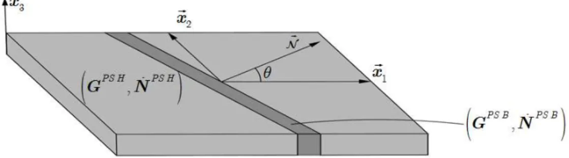
Figure 3 illustrates the localization of deformation in a metal sheet, which is represented by a locali-zation band defined by its unit normal vector .
Figure 3: Illustration of localized necking in a metal sheet.
In the current study, the three-dimensional formulation of the bifurcation approach implemented in Franz et al. (2009a, 2013) is adapted to the plane-stress framework. With the plane-stress condition, the nominal stress rate tensor and the velocity gradient satisfy the following mixed boundary condi-tions:
1 0 0 ? ? 0
0 0 ; ? ? 0
0 0 ? 0 0 0
r
æ ö÷ æ ö÷
ç ÷ ç ÷
ç ÷ ç ÷
ç ÷ ç ÷
=çç ÷÷ =çç ÷÷
÷ ÷
ç ÷ ç ÷
ç ÷ ç ÷
ç ç
è ø è ø
G N (40)
where r is the strain-path parameter, and symbol
?
designates the unknown components. Though in the present work the adopted tangent modulus is different from that developed in Franz et al. (2009a, 2013), the bifurcation criterion has the same formdet ( .PS.)= 0 (41)
where PS
is the 2D tangent modulus that relates the in-plane components of the nominal stress rate tensor to the in-plane components of the velocity gradient. The analytical expression for the 2D tangent modulus PS
is derived from the general expression of the 3D tangent modulus
by the classical relation33 33 3333
, , , 1 2 :, abgdPS abgd ab gd
a b g d
" =
=
-
5 NUMERICAL RESULTS AT THE MACROSCALE
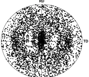
In this section, we investigate the influence of both flow rules (namely, the CSL and the RSL models) on the overall stress–strain responses as well as on the predicted FLDs at the polycrystal scale. As a starting point, an FCC polycrystalline aggregate composed of 1000 grains is considered. The hardening parameters as well as the elastic constants are the same as those used in Section 2.3. Figure 4 shows the random initial texture taken for this polycrystal.
Figure 4: {111} Pole figure for the initial texture (1000 grains).
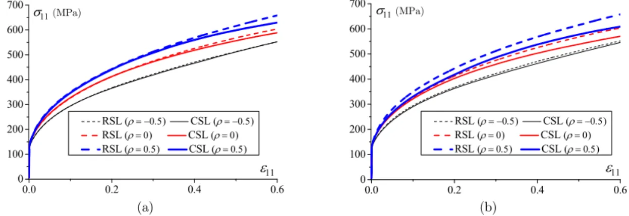
Figure 5 compares the stress–strain responses, obtained with both flow rules, for three different in-plane strain paths r: uniaxial tensile test (r= -0.5), plane-strain tension (r=0), and positive biaxial stretching (r=0.5). For the RSL, the regularization parameter n that measures the sharpness
of the corresponding yield surface is set to 20. This value is motivated by a reasonable compromise between the computation time and the stress–strain curve matching of both flow rules. Indeed, the computation time increases significantly with the value of n, because the time step requires to be
divided into several sub-increments in order to accurately satisfy the yield criterion. For all the com-putations related to the RSL presented hereafter, parameter n is fixed to 20. In Figure 5(a), the
Taylor model is used as homogenization scheme. From this figure, one can observe that at large strains, the gap between the RSL and the CSL-based responses increases as the strain-path parameter r increases. However, in the small strain range, it is found that both flow rules yield the same re-sponse, as previously mentioned by Yoshida et al. (2009). In Figure 5(b), the SC model is used to assess the macroscopic behavior of the material. In this latter case, except for the uniaxial tensile test, the deviations between the RSL and CSL occur at much earlier stage of deformation, with a softer response yielded by the CSL. On the other hand, comparisons between the Taylor model and the SC scheme (see, e.g., Figures 5(a) and 5(b)) reveal that the use of the RSL leads to the same overall stress–strain response, irrespective of the homogenization model, whereas the use of CSL leads to a softer response with the SC approach. These observations are fully consistent with those made by Yoshida et al. (2009).
(a) (b)
Figure 5: Overall stress–strain responses for three different in-plane loading paths: (a) Taylor model; (b) Self-consistent model.
Figure 6 depicts the evolution of some components of the tangent modulus as function of the major strain. It is well-known that the incremental elasto-plastic tangent modulus plays a major role in the framework of bifurcation theory. In this regard, the evolution of the components
1111,
1122,and
1212, which are representative of the other components, is investigated. It is worth noting that, in the case of RSL, the predicted components keep their high elastic values in the course of loading. Quite the opposite trend is observed with the CSL, where the shearing components of the tangent modulus, represented by
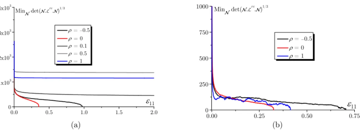
1212, are significantly reduced beyond the elastic range of deformation. In spite of this significant reduction in the shear components, notice that the stress–strain responses yielded by both flow rules are practically the same with the Taylor model (see, e.g., Figure (5)).Figures 7 and 8 show the evolution of the minimum of the determinant of the acoustic tensor, over all possible band orientations, as a function of the major strain, for different strain paths. In Figure 7, the Taylor model is used as scale-transition scheme. Recall that strain localization is marked by the singularity of the acoustic tensor (i.e., as soon as its determinant reaches zero). In the range of negative strain paths (see, e.g., r= -0.5 and r=0), we observe a quasi-continuous drop in the determinant of the acoustic tensor, for both flow rules, which regularly decreases and eventually reaches zero. However, for positive strain paths (r>0), the trend is completely different for the RSL framework, in which the determinant decreases very slightly for r=0.1 and keeps practically a constant value for r =1 or r=0.5. As discussed in the literature, most often within phenomeno-logical constitutive frameworks (see, e.g., Rice, 1976; Hutchinson and Neale, 1978; Ben Bettaieb and Abed-Meraim, 2015), it is found that when the shearing components of the tangent modulus keep their high elastic values, the use of bifurcation theory as localization criterion yields unrealistically high localization strains in the positive biaxial stretching range. Here, the localization predictions suggest values for the critical strains far beyond 2. In Figure 8, the same analysis as that conducted in Figure 7 is followed, but with the SC model as homogenization scheme. As can be observed, the SC approach (see Figure 8) reveals trends quite similar to those reflected by the Taylor model. Be-sides, for the CSL, the predicted localization strains given by the SC model are much lower in the
0.0 0.2 0.4 0.6
0 100 200 300 400 500 600 700
(MPa)
RSL () CSL () RSL () CSL () RSL () CSL ()
0.0 0.2 0.4 0.6
0 100 200 300 400 500 600 700
RSL () CSL () RSL () CSL () RSL () CSL ()
(MPa)
whole than those obtained with the Taylor model. For the RSL, however, there are no significant differences between the Taylor and the SC localization predictions.
(a) (b)
(c) (d)
(e) (f)
Figure 6:Evolution of the components of the tangent modulus for different strain paths: (a) Taylor model (r= -0.5); (b) SC model (r= -0.5); (c) Taylor model (r=0); (d) SC model (r=0);
(e) Taylor model (r=0.5); (f) SC model (r=0.5).
0.0 0.2 0.4 0.6
0 1x10⁵
2x10⁵
3x10⁵
RSL (1111) CSL (1111) RSL (1122) CSL (1122) RSL (1212) CSL (1212)
0.0 0.2 0.4 0.6
0 1x10⁵
2x10⁵
3x10⁵
4x10⁵
RSL (1111) CSL (1111) RSL (1122) CSL (1122) RSL (1212) CSL (1212)
0.0 0.2 0.4 0.6
0 1x10⁵
2x10⁵
3x10⁵
4x10⁵
RSL (1111) CSL (1111)
RSL (1122) CSL (1122)
RSL (1212) CSL (1212)
0.0 0.2 0.4 0.6
0 1x10⁵
2x10⁵
3x10⁵
RSL (1111) CSL (1111) RSL (1122) CSL (1122) RSL (1212) CSL (1212)
0.0 0.2 0.4 0.6
0 1x10⁵
2x10⁵
3x10⁵
4x10⁵
RSL (1111) CSL (1111)
RSL (1122) CSL (1122) RSL (1212) CSL (1212)
0.0 0.2 0.4 0.6
0 1x10⁵
2x10⁵
3x10⁵
4x10⁵
RSL (1111) CSL (1111)
RSL (1122) CSL (1122)
RSL (1212) CSL (1212)
(a) (b)
Figure 7: Evolution of the minimal determinant of the acoustic tensor for different strain paths: (a) RSL (n=20) coupled with the Taylor model; (b) CSL coupled with the Taylor model.
(a) (b)
Figure 8: Evolution of the minimal determinant of the acoustic tensor for different strain paths: (a) RSL (n=20) coupled with the SC model; (b) CSL coupled with the SC model.
Figure 9 displays the localized necking strains predicted for all of the strain paths ranging from uniaxial tension (r= -0.5) to equibiaxial expansion (r=1). The two homogenization models (namely, the Taylor and SC scale-transition schemes) are coupled with both plastic flow rules (i.e., CSL and RSL). As previously mentioned, the limit strains predicted by the RSL are extremely high in the range of positive in-plane biaxial stretching. This trend is consistent with the observations made in Figure 6, where it was shown that the shearing components of the tangent modulus keep their elastic values when the RSL is used, which leads to unrealistically high limit strains in the positive biaxial stretching range. In the negative strain-path range, however, the RSL necking strains are predicted at realistic levels, although they are much higher than those obtained with the CSL (see Figure 9).
0.0 0.5 1.0 1.5 2.0
0 1x10³ 2x10³ 3x10³ 4x10³
11 Min det(.PS
.)1/3
= -0.5 = 0
= 0.1
= 0.5
= 1
0.00 0.25 0.50 0.75 0
250 500 750 1000
11
Min det(.PS
.)1/3
= -0.5 = 0 = 1
0.0 0.5 1.0 1.5 2.0
0 1x10³ 2x10³ 3x10³ 4x10³
11 Min det(.PS
.)1/3
= -0.5
= 0
= 0.1
= 0.5
= 1
0.00 0.25 0.50 0.75 0
250 500 750 1000
11
Min det(.PS
.)1/3
(a) (b)
Figure 9: FLDs predicted by the two different homogenization models for both plastic flow rules: (a) Taylor model; (b) SC model.
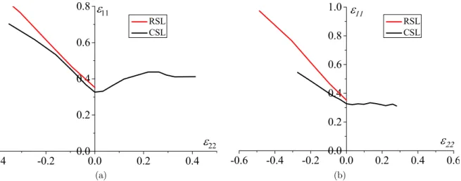
Figure 10 shows the evolution of the localization band orientation, corresponding to the predicted FLDs, as function of the strain-path parameter r. With the Taylor model, the predicted band orien-tations are almost the same for both plastic flow rules in the range of negative strain paths (r<0) (see Figure 10(a)). For the SC model, however, the differences in terms of predicted band orientations are more noticeable in the range of negative strain paths (see Figure 10(b)). Also, with the SC ap-proach, and for the studied polycrystalline aggregate (see its initial texture shown in Figure 4), the localization bands predicted by the CSL are found to remain always normal to the major strain direction in the range of positive strain paths (r>0).
(a) (b)
Figure 10: Critical band orientations as predicted by: (a) Taylor model; (b) SC model.
6 CONCLUDING REMARKS
The effect of the plastic flow rule, as modeled at the single crystal scale, on the forming limit diagrams of polycrystalline sheet metals has been investigated using the bifurcation approach as localization criterion. To this end, two different plastic flow rules have been considered at the single crystal scale.
-0.4 -0.2 0.00.0 0.2 0.4
0.2 0.4 0.6 0.8
RSL CSL
-0.6 -0.4 -0.2 0.00.0 0.2 0.4 0.6
0.2 0.4 0.6 0.8 1.0
RSL CSL
-0.4 -0.2 0.0 0.2 0.4 0.6 0.8 1.0 0
5 10 15 20 25 30 35 40
RSL CSL (°)
-0.4 -0.2 0.0 0.2 0.4 0.6 0.8 1.0 0
5 10 15 20 25 30 35 40
(°)
The first one is based on the classical Schmid law, which results in a yield surface with sharp vertices, while the other uses a regular form of the Schmid law, which leads to a smoother yield surface (i.e., with rounded vertices). In both cases, the Taylor model as well as the self-consistent scale-transition scheme are used to relate the micro and macro scales. From the numerical results, it is found that, in the range of negative strain paths, the FLDs predicted by the regularized Schmid law are realistic, although much higher than those predicted by the classical Schmid law, and this conclusion is valid irrespective of the scale-transition scheme considered (Taylor model or incremental self-consistent approach). However, in the range of positive strain paths, the predicted limit strains given by the regularized Schmid law are unrealistically high, in contrast to those obtained by the classical Schmid law, which remain quite realistic. It is also found that when the regularized Schmid law is used, the overall stress–strain response of the material as well as the predicted necking strains are almost in-sensitive to the scale-transition scheme, at variance with the use of the classical Schmid law.
References
Abed-Meraim, F., Balan, T., Altmeyer, G. (2014). Investigation and comparative analysis of plastic instability criteria: application to forming limit diagrams. International Journal of Advanced Manufacturing Technology 71:1247–1262. Asaro, R.J., Needleman, A. (1985). Texture development and strain hardening in rate dependent polycrystals. Acta Metallurgica 33:923–953.
Ben Bettaieb, M., Abed-Meraim, F. (2015). Investigation of localized necking in substrate-supported metal layers: Comparison of bifurcation and imperfection analyses. International Journal of Plasticity 65:168–190.
Bunge, H.J. (1968). The orientation distribution function of the crystallites in cold rolled and annealed low-carbon steel sheets. Physica Status Solidi (b) 26:167–172.
Considère, A. (1885). Mémoire sur l’emploi du fer et de l’acier dans les constructions. Annales des Ponts et Chaussées 9:574–775.
Drucker, D.C. (1950). Some implications of work hardening and ideal plasticity. Quarterly ofApplied Mathematics 7:411–418.
Drucker, D.C. (1956). On the uniqueness in the theory of plasticity. Quarterly ofApplied Mathematics 16:35–42. Dudzinski, D., Molinari, A. (1991). Perturbation analysis of thermoviscoplastic instabilities in biaxial loading. International Journal of Solidsand Structures 27:601–628.
Franz, G., Abed-Meraim, F., Ben Zineb, T., Lemoine, X., Berveiller, M. (2009b). Strain localization analysis using a multiscale model. Computational Materials Science 45:768–773.
Franz, G., Abed-Meraim, F., Berveiller, M. (2013). Strain localization analysis for single crystals and polycrystals: Towards microstructure-ductility linkage. International Journal of Plasticity 48:1–33.
Franz, G., Abed-Meraim, F., Lorrain, J.P., Ben Zineb, T., Lemoine, X., Berveiller, M. (2009a). Ellipticity loss analysis for tangent moduli deduced from a large strain elastic–plastic self-consistent model. International Journal of Plasticity 25:205–238.
Gambin, W. (1992). Refined analysis of elastic–plastic crystals. International Journal of Solidsand Structures 29:2013– 2021.
Gambin, W., Barlat, F. (1997). Modeling of deformation texture development based on rate independent crystal plas-ticity. International Journal of Plasticity 13:75–85.
Haddag, B., Abed-Meraim, F., Balan, T. (2009). Strain localization analysis using a large deformation anisotropic elastic–plastic model coupled with damage. International Journal of Plasticity 25:1970–1996.
Hill, R. (1958). A general theory of uniqueness and stability in elastic–plastic solids. Journal of the Mechanics and Physics of Solids 6:239–249.
Hill, R. (1965a). Continuum micro-mechanics of elastoplastic polycrystals. Journal of the Mechanics and Physics of Solids 13:89–101.
Hill, R. (1965b). A self consistent mechanics of composite materials. Journal of the Mechanics and Physics of Solids 13:213–221.
Hutchinson, J.W., Neale, K.W. (1978). Sheet Necking – II. Time-independent behavior. In: D.P. Koistinen, N.M. Wang (Eds.), Mechanics of sheet metal forming. New York: Plenum Press, 127–153.
Imbault, D., Arminjon, M. (1998). Deformation textures of fcc materials predicted with a regular form of the Schmid law. Materials Science Forum 273:371–376.
Keeler, S.P., Backofen, W.A. (1963). Plastic instability and fracture in sheets stretched over rigid punches. Trans. ASM 56:25–48.
Lipinski, P., Berveiller, M. (1989). Elastoplasticity of micro-inhomogeneous metals at large strains. International Jour-nal of Plasticity 5:149–172.
Lipinski, P., Berveiller, M., Reubrez, E., Morreale, J. (1995). Transition theories of elastic–plastic deformation of metallic polycrystals. Archive of Applied Mechanics 65:291–311.
Mansouri, L.Z., Chalal, H., Abed-Meraim, F. (2014). Ductility limit prediction using a GTN damage model coupled with localization bifurcation analysis. Mechanics of Materials 76:64–92.
Marciniak, Z., Kuczynski, K. (1967). Limit strains in processes of stretch-forming sheet metal. International Journal of Mechanical Sciences 9:609–620.
Molinari, A., Clifton, R. (1987). Analytical characterization of shear localization in thermo-visco-plastic solids. Journal of Applied Mechanics 54:806–812.
Rice, J.R. (1976). The localization of plastic deformation. In: 14th International Congress of Theoretical and Applied Mechanics 207–220.
Schmid, E., Boas, W. (1935). Plasticity of Crystals. Chapman and Hall, London.
Stören, S., Rice, J.R. (1975). Localized necking in thin sheets. Journal of the Mechanics and Physics of Solids 23:421– 441.
Appendix A
The set of FCC slip systems is given in the table below:
a 1 2 3 4 5 6
0
3m a [0 –1 1] [1 0 1] [1 1 0] [0 –1 1] [–1 0 1] [1 –1 0]
0
2n a (–1 1 1) (–1 1 1) (–1 1 1) (1 1 1) (1 1 1) (1 1 1)
a 7 8 9 10 11 12
0
3m a [0 1 1] [1 0 1] [1 –1 1] [0 1 1] [–1 0 1] [1 1 0]
0
2n a (1 1 –1) (1 1 –1) (1 1 –1) (1 –1 1) (1 –1 1) (1 –1 1)
Table A.1: List of FCC slip systems related to the intermediate configuration.
The hardening matrix used in this study is of power-law type, which is given by the following relations:
1 1 0 0
0 1 0 1
1 ;
g
t N n
h
H h dt
n
ab a
a g t
-=
æ G ö÷
ç
= ççè + ÷÷ø G =
ò
å
(A.1)where