a New Methodology to Find Initial Solution for Problems

(1)

http://dx.doi.org/10.12988/ams.2015.4121013

The MOMC Method: a New Methodology to Find

Initial Solution for Transportation Problems

Giancarlo de França Aguiar

Federal Institute of Paraná and Positivo University, Street João Negrão Post box 1285, Curitiba- Paraná, 80230-150, Brazil

Bárbara de Cássia Xavier Cassins Aguiar

Federal University of Paraná - DEGRAF, Jardim das Américas Post box 19081, Curitiba- Paraná, 81531-980, Brazil

Volmir Eugênio Wilhelm

Federal University of Paraná - DEGRAF, Jardim das Américas Post box 19081, Curitiba- Paraná, 81531-980, Brazil

Copyright © 2014 Giancarlo de França Aguiar et al. This is an open access article distributed under the Creative Commons Attribution License, which permits unrestricted use, distribution, and reproduction in any medium, provided the original work is properly cited.

Abstract

In this paper we propose a new algorithm for finding a feasible initial solution for transportation problems. The MOMC Method (Maximum Supply with Minimum Cost) as it was called was compared with three classical methods: Corner Northwest, Minimum Cost and Vogel, obtaining significant results (better or equal to the presented methods). A numerical example was presented to a rigorous understanding of the algorithm, and the results showed great computational advantage (higher processing speed and less memory usage), with up to 99.86% gains by initial decision-making.

Keywords: Transportation Problem, MOMC Method, Feasible Initial Solution

1 Introduction

(2)

902 Giancarlo de França Aguiar et al.

of the first basic problems of transportation. Appa in 1973 [1] discussed several variations of the transportation problem. The solution to many of these problems can be found using the simplex method, for example with teachers Charnes and Cooper [4] in 1954, and Dantzig Thapa [5] in 1963 and Arsham and Khan [2] in 1989, but because of its very particular mathematical structure, new approaches have been proposed and studied.

The simplex method is an iterative algorithm, it requires an initial feasible solution to the problem. The four main classical methods, very widespread in the literature for finding an initial solution are: the north-west corner method (see Zionts [20] in 1974), Vogel method (see Murty [10] in 1983), the Cost Minimum method (see Puccinni and Pizzolato [11] in 1987) and Russell's method (see Ruiz and Landín [14] in 2003) each with its own advantages, disadvantages and particularities. However researchers as Rodrigues [12] has proposed and studied new approaches to find an initial solution to transportation problems.

Armed with an initial solution, the new goal becomes: find out if this solution is optimal or not. Several heuristics as in Kaur and Kumar [9] in 2011, Silva [16] in 2012, Samuel and Venkatachalapathy [15] in 2013 and Ebrahimnejad [6] in 2014, have been developed to find an optimal solution to transportation problems, from an initial feasible solution. These new heuristics have gotten increasingly satisfactory results (more efficient algorithms) and with various practical applications.

Another branch of very exploited Transportation problems, and that has become increasingly important in scientific circles, are the problems involving inaccuracies in the collection and treatment of measures of cost factors, supply and demand, and that many of these measures are uncontrollable, requiring then the use of fuzzy logic in dealing and development of these new techniques. The pioneers in the study of fuzzy environment in decision-making were the researchers Zadeh [19] and Bellmann and Zadeh [3] in 1965 and 1970 respectively. Following this work, new authors as Tanaka and Asai [18] in 1984, Rommelfanger, Wolf and Hanuscheck [13] in 1989, Fang Hu, Wang and Wu [7] in 1999, Sudha, Margaret and Yuvarani [17] in 2014 have developed fuzzy linear programming techniques to transportation problems.

However, the initial solution has been little exploited, probably because efficiency of the traditional methods and also by extensive computational power of modern computers, which easily rotate the simplex method to a problem with a large number of variables and constraints.

(3)

2 Transportation Problem

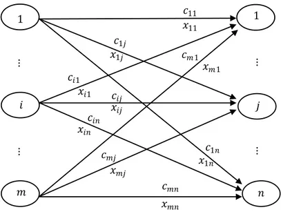
Following we see the transportation problem in their tabular form (in a table 2.1), as a linear programming model and as a network model.

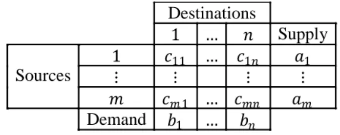
TABLE 2.1: Tabulated Form for to Transportation Problem

Destinations

1 … Supply

Sources

1 ₁₁ … ₁ ₁

⋮ ⋮ ⋮ ⋮

1 …

Demand ₁ …

Inserted in linear programming, the transportation model deserves special attention, having its own characteristics and a general model:

n ,..., j e m ,..., i , x ) Demand ( n ,..., j , b x ) Supply ( m ,..., i , a x : . a . s x . c C Min ij j m i ij i n j ij m i n j ij ij 1 1 0 1 1 1 1 1 1        





   

(4)

1 1

⋮

11

�11 1

�1

1

�1 1

�1

� �

1

� 1

�

FIGURE 2.1: Network for the Transportation Problem

3 Initial Solution for Transportation Problems

There are three classic models very worked in the literature to find an initial solution to transportation problems. The North-west Corner Method, the Minimum Cost Method and Vogel Method.

3.1 The North-west corner method

The North-west corner method (can be evaluated in Zionts [20]) as it is known does not consider transport costs in decision-making, depending only on the supply and demand of the origins and destinations respectively and having relatively simple computational development. In general your solution is not as efficient (near optimal), but its application is a feasible solution.

3.2 Minimum Cost Method

The Minimum Cost Method as the name suggests is based on an analysis of transport costs and also the examination of the values of supply and demand, aiming a closer initial solution of the optimal than that provided by the Northwest Corner Method. A detailed study of the method can be seen in Puccini and Pizzolato [11] in 1987.

3.3 Vogel Method

(5)

this method, each transmission frame must be calculated for each row and each column, the difference between the two lower cost, the result is called penalty. In the column or row where the biggest difference occurs choose the cell, called basic cell, which has the lowest value. The algorithmic process can be seen in Murty [10] in 1983.

3.4 New Methodology

This paper proposes a new methodology to find a feasible initial solution to transportation problems. The Maximum Offer Method with Minimum Cost or MOMC will be named as described in the following algorithm.

3.4.1 The MOMC Algorithm

The following steps are illustrated to find a feasible initial solution for a balanced transportation problem, that is, where the supply of origins is equal to demand of destinations.

Step 1: Select i line with the highest supply ( ); If a tie, choose the line that has the lowest cost;

Step 2: In line with the increased supply of step 1, choose the column with the lowest cost ( ); If a tie, choose the column j with the highest demand;

Step 3: The cell intersection of the line (step 1) with the column (step 2) is selected;

Step 4: Allocate the maximum supply (quantity) of step 1 line to the cell ( ) selected, up to the amount of demand j column;

Step 5: Decrease of the supply (line i) and Demand (column j) the amount allocated to the cell ( ) from step 4;

If demand < supply, then the demand is annulled; If demand > suply, then the supply will be annulled;

If demand = supply, then the demand and the supply is annulled;

Step 6: Eliminate of the transportation model (Table), the column or line with demand or supply annulled after step 5; If demand (column) and supply (line) are zero simultaneously, then eliminate them;

(6)

4 Numerical Example

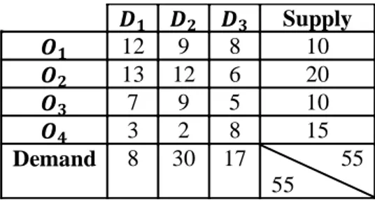
This time will be shown how to find an initial solution for a transportation problem using the MOMC Algorithm. Consider the following balanced transportation problem with four origins and three destinations simplistic just to didactic purpose of applying MOMC algorithm, as shown in Table 4.1.

TABLE 4.1: Numerical example

� � � Supply

� 12 9 8 10

� 13 12 6 20

� 7 9 5 10

� 3 2 8 15

Demand 8 30 17 55

55

Let's consider how line 1, the corresponding line source 1 and consider how column 1, the column corresponding to the target 1. The following is illustrated the development of the 7 steps of the first iteration.

Step 1: Select i line with the highest supply ( ); If a tie, choose the line that has the lowest cost:

The line with the highest supply (20) is the line 2.

Step 2: In line with the increased supply of step 1, choose the column with the lowest cost ( ); If a tie, choose the column j with the highest demand:

The column of line 2 with lower cost (6) is the column 3.

Step 3: The cell intersection of the line (step 1) with the column (step 2) is selected:

The corresponding cell is , as shown in Table 4.2 below.

TABLE 4.2: Choice of cell

� � � Supply

� 12 9 8 10

� 13 12 6 20

� 7 9 5 10

� 3 2 8 15

Demand 8 30 17 55

(7)

Step 4: Allocate the maximum supply (quantity) of step 1 line to the cell ( ) selected, up to the amount of demand j column:

The source 2 can supply 20 units, however the destination 3 requires 17 units. So will be allocated 17 units from the origin to the destination 3. .

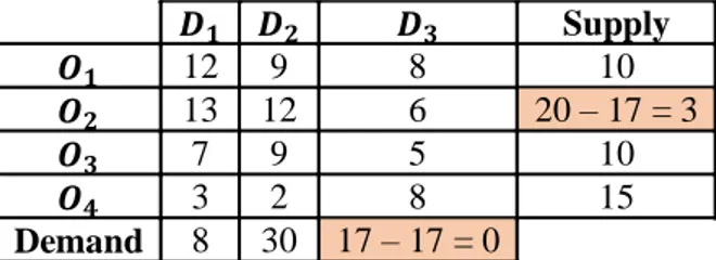
Step 5: Decrease of the supply (line i) and Demand (column j) the amount allocated to the cell ( ) from step 4:

The following Table 4.3 illustrates step 5.

TABLE 4.3: Step 5

� � � Supply

� 12 9 8 10

� 13 12 6 20 – 17 = 3

� 7 9 5 10

� 3 2 8 15

Demand 8 30 17 – 17 = 0

Step 6: Eliminate of the transportation model (Table), the column or line with demand or supply annulled after step 5; If demand (column) and supply (line) are zero simultaneously, then eliminate them:

As the demand of the target 3 was annulled, then leaves the frame column 3, as shown in Table 4.4 below.

TABLE 4.4: Reduced Numerical Example

� � Supply

� 12 9 10

� 13 12 3

� 7 9 10

� 3 2 15

Demand 8 30

Step 7: If there no more supply, end. Otherwise, return to step 1, starting the next iteration.

(8)

908 Giancarlo de França Aguiar et al.

Iteration: 2 (A cell x_42 = 15)

FIGURE 4.1: Iteration 2

Iteration: 3 (A cell )

� � Supply

� 12 9 10

� 13 12 3

� 7 9 10

� 3 2 15

Demand 8 30

� � Supply

� 12 9 10

� 13 12 3

� 7 9 10

� 3 2 15 - 15 = 0

Demand 8 30 – 15 = 15

� � Supply

� 12 9 10

� 13 12 3

� 7 9 10

Demand 8 15

� � Supply

� 12 9 10

� 13 12 3

� 7 9 10

Demand 8 15

� � Supply

� 12 9 10

� 13 12 3

� 7 9 10 – 8 = 2

Demand 8 – 8 = 0 15

� Supply

� 9 10

� 12 3

� 9 2

Demand 15

� Supply

� 9 10 – 10 = 0

� 12 3

� 9 2

Demand 15 – 10 = 5

� Supply

� 9 10

� 12 3

� 9 2

(9)

5 Results

Will be presented at this time the results of the application of the North-west Corner Method, of Minimum Cost Method, Vogel method and MOMC method for the numerical example of the previous section. Table 5.1 shows the results.

� Supply

� 12 3

� 9 2

Demand 5

� Supply

� 12 3

� 9 2

Demand 5

� Supply

� 12 3 – 3 = 0

� 9 2

Demand 5 – 3 = 2

� Supply

� 9 2

Demand 2

� Supply

� 9 2 – 2 = 0

Demand 2 – 2 = 0

� Supply

� 9 2

(10)

910 Giancarlo de França Aguiar et al.

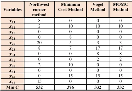
TABLE 5.1: Results of Numerical Example

Variables

Northwest corner method

Minimum Cost Method

Vogel Method

MOMC Method

� 8 0 0 0

� 2 10 10 10

� 0 0 0 0

� 0 8 0 0

� 20 5 3 3

� 8 7 17 17

� 0 0 8 8

� 0 0 2 2

� 2 10 0 0

� 0 0 0 0

� 0 15 15 15

� 15 0 0 0

Min C 532 376 332 332

The application of the Northwest Corner method shows the following results:�11 = 8,�12 = 2,�22 = 20,�23 = 8,�33 = 2 e �43 = 15. The other variables are null. Once the minimum cost function returns � � = 12 8 + 9 2 + 8 0 + 13 0 + 12 20 + 6 8 + 7 0 + 9 0 + 5 2 + 3 0 + 2 0 + 8 15 = 532.

The use of the Minimum Cost Method presents the results: �42 = 15, �33 = 10, �₂₃ = 7,�₁₂ = 10,�₂₂ = 5 e �21 = 8.

The remaining variables have zero value, and the minimum cost function returns

� �= 12 0 + 9 10 + 8 0 + 13 8 + 12 5 + 6 7 + 7 0 + 9 0 +

5 10 + 3 0 + 2 15 + 8 0 = 376. This method was a better result (lower cost) than the Northwest Corner method, however, is still not the best.

The use of the Vogel method yielded the following results: �23 = 17,�42 = 15,�₃₁ = 8,�₁₂ = 10,�₂₂ = 3 e �32 = 2. The other variables are null. The

(11)

The MOMC method showed the following results: �23 = 17,�42 = 15,�31 = 8,�₁₂ = 10,�₂₂ = 3and �32 = 2. The other variables are null. Thus, the minimum cost function resulted in � �= 12 0 + 9 10 + 8 0 + 13 0 + 12 3 + 6 17 + 7 8 + 9 2 + 5 0 + 3 0 + 2 15 + 8 0 = 332, better than the Northwest corner method, better than the Minimum Cost Method and with the same result (optimal) the method Vogel.

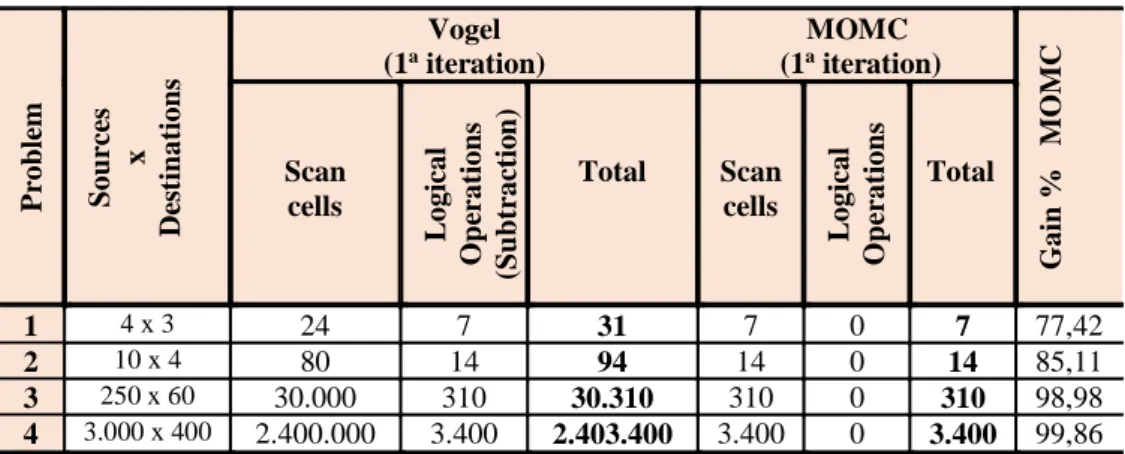
The great advantage of using MOMC method is not only a good approximation (in the previous example has found the optimal solution) of the optimal solution, but the computational time to solve problems. The following table 5.2 illustrates a simulation of the scan cells and logical operations performed by a computer.

TABLE 5.2: Comparison of the Vogel method with the MOMC method

P rob lem S ou rc es x De st in at ion s Vogel

(1a_iteration)

MOMC

(1a_iteration)

Ga in % M OMC Scan cells L ogical Op er at ion s (S u b tr ac tio n )

Total Scan

cells L ogical Op er at ion s Total

1 4 x 3 24 7 31 7 0 7 77,42

2 10 x 4 80 14 94 14 0 14 85,11

3 250 x 60 30.000 310 30.310 310 0 310 98,98

4 3.000 x 400 2.400.000 3.400 2.403.400 3.400 0 3.400 99,86

Analyzing a problem with four sources and three destinations, the Vogel method scans on 12 horizontal cells, more vertical cells 12 to determine the two lowest costs each row and each column (a total of 24 cells). It performs four logical operations (difference between the lowest costs) in the horizontal and 3 vertical operations (a total of 4 operations). Performing in total 31 decisions, only in the first iteration.

(12)

6 Conclusions

This paper presented a new algorithm called MOMC method. This method has shown significant advantages in simplifying calculations and decision making to find an initial solution to transportation problems.

In many worked examples by author so far, the MOMC method has proven effective finding the optimal solution without the need for optimality algorithm.

From the computational point of view (higher processing speed and less memory usage), the example text could illustrate the efficiency of capacity MOMC method with up to 99.86% gains even in the first iteration with respect to Vogel method (one the most implemented according to the literature).

The next work will be the implementation (in language with graphical programming interface), computer simulation of classical problems, and its extension to transportation problems with parameters (cost, supply and demand) fuzzy.

References

[1] Appa. G. M. The transportation problem and its variants. Oper. Res. Quart. 24: 79-99, (1973). http://dx.doi.org/10.1057/jors.1973.10

[2] Arsham, H., Khan, A. B. A simplex-type algorithm for general transportation problems: An alternative to stepping-stone. J. Oper. Res. Soc. 40: 581-590, (1989). http://dx.doi.org/10.1057/jors.1989.95

[3] Bellmann, R. E., Zadeh, L. A. Decision making in fuzzy environment, Management sciences, 17, 141-164, (1970).

http://dx.doi.org/10.1287/mnsc.17.4.b141

[4] Charnes, A., Cooper, W.W. The stepping-stone method for explaining linear programming calculation in transportation problem. Management Sci. 1, 49-69, (1954). http://dx.doi.org/10.1287/mnsc.1.1.49

[5] Dantzig, G. B., Thapa, M. N. Springer: Linear Programming: 2: Theory and Extensions. Princeton University Press, New Jersey, 1963.

(13)

[7] Fang, S. C., Hu, C. F., Wang, H.F., Wu, S. Y. Linear programming with fuzzy coefficients in constraints, Computers and mathematics with applications, 37, 63-76, (1999). http://dx.doi.org/10.1016/s0898-1221(99)00126-1

[8] Hitchcock, F. L. The distribution of a product from several sources to numerous localities. J. Math. Phys. 20: 224-230, (1941).

[9] Kaur, A., Kumar, A. A new method for solving fuzzy transportation problems using ranking function. Applied Mathematical Modelling 35, 5652-5661, (2011). http://dx.doi.org/10.1016/j.apm.2011.05.012

[10] Murty, G. Linear Programming. Wiley, New York: John Wiley e Sons,1983.

[11] Puccini, A. L., Pizzolato, N.D. Linear Programming. Rio de Janeiro, 1987.

[12] Rodrigues, M. M. E. M. Transportation method: development of a new initial solution. Journal of Business Administration. vol.15, no. 2, São Paulo Mar. / Apr. 1975.

[13] Rommelfanger, H., Wolf, J., Hanuscheck, R. Linear programming with fuzzy coefficients, Fuzzy sets and systems, 29, 195-206, (1989).

[14] Ruiz, F.L., Landín, G.A. Nuevos Algoritmos em el Problema de Transporte. V Congreso de Ingeniería de Organización. Valladolid-Burgos, p. 4-5, setembro, 2003.

[15] Samuel, A. E., Venkatachalapathy, M. A simple heuristic for solving generalized fuzzy transportation problems. International Journal of Pure and Applied Mathematics, vol. 83, n. 1, 91-100, (2013).

http://dx.doi.org/10.12732/ijpam.v83i1.8

[16] Silva, T. C. L. New methodology for solving transportation problems in sparse cases. Doctoral Thesis. PPGMNE, (2012).

[17] Sudha, S., Margaret, A. M., Yuvarani, R. A New Approach for Fuzzy Transportation Problem, International Journal of Innovative Research and Studies, April, 2014, Vol3, Issue 4, 251-260.

[18] Tanaka, H. I. and Asai, K. A formulation of fuzzy linear programming based on comparison of fuzzy numbers, Control and Cybernetics, 13, 185-194, (1984).

(14)

[20] Zionts, S. Linear and integer programming. Englewood Cliffs, New Jersey, Prentice Hall, 1974.