www.hydrol-earth-syst-sci.net/18/4979/2014/ doi:10.5194/hess-18-4979-2014
© Author(s) 2014. CC Attribution 3.0 License.
Evaluation of root water uptake in the ISBA-A-gs land surface
model using agricultural yield statistics over France
N. Canal1,2, J.-C. Calvet1, B. Decharme1, D. Carrer1, S. Lafont1,*, and G. Pigeon3
1CNRM-GAME – UMR3589, Météo-France, CNRS, Toulouse, France
2ARVALIS Institut du végétal, Service Systèmes d’Information et Méthodologies, Boigneville, France 3Météo-France, Division Agrométéorologie, Toulouse, France
*now at: ISPA – UMR1391, INRA, Villenave d’Ornon, France Correspondence to:J.-C. Calvet ([email protected])
Received: 5 May 2014 – Published in Hydrol. Earth Syst. Sci. Discuss.: 23 May 2014 Revised: 2 November 2014 – Accepted: 12 November 2014 – Published: 10 December 2014
Abstract. The simulation of root water uptake in land sur-face models is affected by large uncertainties. The difficulty in mapping soil depth and in describing the capacity of plants to develop a rooting system is a major obstacle to the simula-tion of the terrestrial water cycle and to the representasimula-tion of the impacts of drought. In this study, long time series of agri-cultural statistics are used to evaluate and constrain root wa-ter uptake models. The inwa-ter-annual variability of cereal grain yield and permanent grassland dry matter yield is simulated over France by the Interactions between Soil, Biosphere and Atmosphere, CO2-reactive (ISBA-A-gs) generic land surface
model (LSM). The two soil profile schemes available in the model are used to simulate the above-ground biomass (Bag)
of cereals and grasslands: a two-layer force–restore (FR-2L) bulk reservoir model and a multi-layer diffusion (DIF) model. The DIF model is implemented with or without deep soil layers below the root zone. The evaluation of the various root water uptake models is achieved by using the French agricultural statistics of Agreste over the 1994–2010 period at 45 cropland and 48 grassland départements, for a range of rooting depths. The number of départements where the sim-ulated annual maximum Bag presents a significant
correla-tion with the yield observacorrela-tions is used as a metric to bench-mark the root water uptake models. Significant correlations (p value<0.01) are found for up to 29 and 77 % of the dé-partements for cereals and grasslands, respectively. A rather neutral impact of the most refined versions of the model is found with respect to the simplified soil hydrology scheme. This shows that efforts should be made in future studies to reduce other sources of uncertainty, e.g. by using a more
de-tailed soil and root density profile description together with satellite vegetation products. It is found that modelling ad-ditional subroot-zone base flow soil layers does not improve (and may even degrade) the representation of the inter-annual variability of the vegetation above-ground biomass. These results are particularly robust for grasslands, as calibrated simulations are able to represent the extreme 2003 and 2007 years corresponding to unfavourable and favourable fodder production, respectively.
1 Introduction
Modelling the land surface processes and the surface energy, water and carbon fluxes is an important field of research in the climate community, as soil moisture and vegetation play an essential role in the climatic Earth system (Seneviratne et al., 2010). Regular improvement and assessment of generic land surface models (LSMs) are also required. In particu-lar, the seasonal and inter-annual variability of the vegeta-tion interacts with hydrological processes, and must be rep-resented well (Szczypta et al., 2012). Modern LSMs such as Interactions between Soil, Biosphere and Atmosphere, CO2-reactive (ISBA-A-gs) (Calvet et al., 1998; Gibelin et
al., 2006) or ORganizing Carbon and Hydrology In Dynamic EcosystEms (ORCHIDEE) (Krinner et al., 2005) are able to simulate the diurnal cycle of water and carbon fluxes and, on a daily basis, plant growth and key vegetation variables such as the above-ground biomass (Bag) and the leaf area
a marked impact on plant growth, and the way root water uptake is represented in such LSMs may influence the sim-ulatedBag and LAI values, in particular the maximum
val-ues reached every year. Therefore, long time series of ob-servations related to the latter quantities, such as agricultural yields, have potential in the evaluation of the simulation of the available soil water content (AWC) and root water up-take in LSMs, provided their inter-annual variability is gov-erned by climate and not by trends or changes in agricultural practices.
In Europe, a marked positive trend in crop yields has been observed in the last 45 years, due to the agricultural intensification and evolution of farming practices (Smith et al., 2010a, b). However, Brisson et al. (2010) and Gate et al. (2010) have shown that yields have been stagnating in Eu-rope since the beginning of the 1990s, and particularly since 1996 in France. Therefore, it can be assumed that in the last two decades, the year-to-year change in the large-scale yield of a given rain-fed crop type is mainly driven by the climate variability. In Europe, Smith et al. (2010a, b) showed that the agricultural statistics can be used to assess crop simula-tions on a country level. On a finer spatial scale over France, Calvet et al. (2012), hereafter referred to as Ca12, have used agricultural statistics (Agreste, 2014) to benchmark several configurations of the ISBA-A-gs LSM through the correla-tion between yield time series and Bag simulations for the
1994–2008 period. The Agreste data are provided for admin-istrative units (hereafter referred to as “départements”). In ISBA-A-gs, the plant phenology is driven by photosynthesis: on a daily basis, plant growth is governed by the accumula-tion of the hourly net assimilaaccumula-tion of CO2 through the
pho-tosynthesis process, and plant mortality is related to a deficit in photosynthesis. The simulated annual maximumBagand
maximum LAI may differ from one year to another in re-lation to the impact of the weather and climate variability on photosynthesis. In regions where a deficit in precipitation may occur, soil moisture is a key driver of the photosynthesis and plant growth of rain-fed crops and grasslands. Although ISBA-A-gs is not a crop model and agricultural practices are not explicitly represented, Ca12 achieved a good represen-tation of the inter-annual variability of the dry matter yield (DMY) for grasslands over many départements in France. On the other hand, representing the year-to-year variability of the grain yield (GY) of winter/spring cereals was more difficult. By performing a sensitivity study on different parameters of the model, they concluded that the maximum available soil water content (MaxAWC) and the mesophyll conductance under well-watered conditions (gm) were the two key
param-eters driving the inter-annual variability of the simulatedBag.
In particular, they showed that the model was markedly sen-sitive to MaxAWC (especially at low MaxAWC values).
In Ca12, an effort was made to benchmark two op-tions of the vegetation model (avoiding vs. drought-tolerant). In this study, an effort is made to benchmark several options of the soil hydrology model. The main objective of
this study is to assess to what extent using more refined rep-resentations of the soil hydrology and the root water uptake can improve the representation of the inter-annual variability of GY (and, possibly, DMY). The ISBA-A-gs model and the method proposed by Ca12 are used to evaluate a new option of the ISBA-A-gs model using a multi-layer soil model per-mitting a more detailed representation of soil moisture and soil temperature profiles, and of root water uptake. Since sev-eral options can be envisaged to implement the multi-layer soil hydrology simulations, a side objective of this study is to benchmark these options and learn about the representation of root water uptake.
The various versions of ISBA-A-gs are presented in Sect. 2, together with the annual yield statistics of Agreste. The symbols used in this work are listed and defined in Ta-ble A1. The results obtained with the different set of simu-lations are shown in Sect. 3 and the differences in the inter-annual variability of the various simulations ofBagare
pre-sented, together with the hydrological variables. The results are analyzed and discussed in Sect. 4 and the conclusions of this study are summed up in Sect. 5.
2 Data and methods
2.1 Agricultural statistics in France
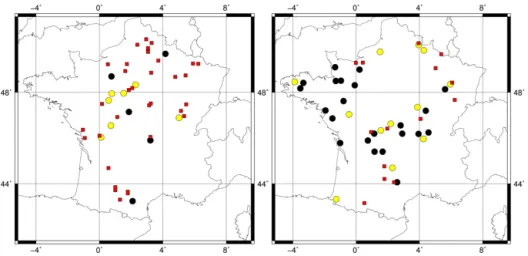
Figure 1.Location of the 45 cropland and 48 grassland 8 km×8 km
grid cells (blue and green dots, respectively) and the corresponding département number.
the rains were abundant over the grassland regions consid-ered in this study, and have also contributed to the higher pro-duction (Agreste Bilans, 2007; Agreste Conjoncture, 2007; Agreste Infos Rapides, 2007).
2.2 The ISBA-A-gs land surface model
The Interactions between Soil, Biosphere, and Atmosphere (ISBA) model (Noilhan and Planton, 1989; Noilhan and Mahfouf, 1996) was designed to describe the daily course of land surface state variables into global and regional climate models, weather forecast models, and hydrological models. In the original version of ISBA, a single root-zone soil layer is considered. A thin top soil layer is represented using the Deardorff (1977, 1978) force–restore approach. Soil charac-teristics, such as soil water and heat coefficients, the wilt-ing point and the field capacity, depend on soil texture (sand and clay fractions). The stomatal conductance calculation is based on the Jarvis (1976) approach, and accounts for photo-synthetically active radiation (PAR), soil water stress, vapour pressure deficit and air temperature.
The representation of the soil physics of the initial version of ISBA was upgraded gradually. A multi-layer soil model including soil freezing processes was developed by Boone et al. (2000) and Decharme et al. (2011). The multi-layer soil model explicitly solves the one-dimensional Fourier law and the mixed form of the Richards equation. The multi-layer representation is used to discretise the total soil profile. In each layer, the temperature and the moisture are computed according to the hydrological and texture layer characteris-tics. The heat and water transfers are decoupled: heat
fer is solely along the thermal gradient, while water trans-fer is induced by gradients in the total hydraulic potential. Hereafter, the two-layer force–restore model and the diffu-sion model are referred to as “FR-2L” and “DIF”, respec-tively.
In addition to the simple Jarvis parameterisation of stomatal conductance, Calvet et al. (1998) and Gibelin et al. (2006) have developed ISBA-A-gs. ISBA-A-gs (“A” stands for net assimilation of CO2, and “gs” for stomatal
conductance) is a CO2-responsive version of ISBA able to
simulate photosynthesis and its coupling to stomatal conduc-tance. This option was used in studies on the impact of cli-mate change (Calvet et al., 2008; Queguiner et al., 2011) and on the impact of drought on the vegetation in the Mediter-ranean basin (Szczypta, 2012).
Under well-watered conditions, the A-gs formulation is based on the model proposed by Jacobs et al. (1996) (Calvet et al., 1998, 2004; Gibelin et al., 2006). In this approach, the main parameter driving photosynthesis isgm. Under
water-limited conditions, a soil moisture stress function (FS) is
ap-plied to key parameters of the photosynthesis model. For herbaceous vegetation, two parameters are assumed to re-spond to soil moisture stress (Calvet, 2000): the mesophyll conductance and the maximum leaf-to-air saturation deficit (Dmax). Low (high) values of the latter correspond to high
(low) sensitivity of the stomatal aperture to air humidity. These photosynthesis parameters are dependent onFS. Two
contrasting responses of the model parameters to soil mois-ture are represented: drought-avoiding and drought-tolerant (see Fig. S1 in the Supplement). WhenFSis higher than the
critical soil water stressFSC(FSC=0.3 in our simulations),
a drop inFStriggers an increase (decrease) ingmand a
de-crease (inde-crease) inDmaxfor the drought-avoiding
(drought-tolerant) parameterisation. The drought-avoiding parameter-isation is used for cereal crops, and the drought-tolerant pa-rameterisation is used for grasslands. This assumption was validated by Ca12. The drought response model is illustrated by Fig. S1. These parameters are then used to calculate the hourly leaf-level net assimilation of CO2 and the stomatal
conductance, in relation to sub-daily meteorological inputs such as the incoming solar radiation. A radiative transfer scheme is then used to upscale net assimilation of CO2and
transpiration at the vegetation level. The plant transpiration flux is used to calculate the soil water budget through the root water uptake. The net assimilation of CO2serves as an
input to the plant growth model, and LAI andBagare updated
on a daily basis. Figure 3 illustrates these mechanisms. For moderate soil water stress, the drought-avoiding response re-sults in an increase in the water use efficiency (WUE). In the drought-tolerant response, WUE does not change, or de-creases. It must be noted that another representation of the response to drought is used for forests (Calvet et al., 2004).
Figure 2.Averaged annual statistics of Agreste over the 1994-2010 period of (top panel) grain yields of six cereals (winter wheat in black, rye in red, winter barley in blue, spring barley in green, oat in orange and triticale in purple) over the 45 départements of Fig. 1 and (bottom panel) dry matter yields of permanent grasslands over the 48 départements of Fig. 1.
Figure 3.Relation of biogeophysical variables to leaf-scale and vegetation-scale fluxes in the ISBA-A-gs simulations.
the above-ground biomass. TheBagvariable has two
com-ponents (active biomass and structural biomass) related by a nitrogen dilution parameterisation (Calvet and Soussana, 2001). The leaf nitrogen concentrationNLis a parameter of
the model affecting the specific leaf area (SLA), the ratio of LAI to leaf biomass (in m2kg−1). The SLA depends onNL
and on plasticity parameters (Gibelin et al., 2006). This ver-sion of ISBA-A-gs, called “NIT”, is used in this study.
An assessment of the quality of ISBA-A-gs output vari-ables has been performed in previous local studies with in situ data over France (Rivalland et al., 2005; de Rosnay et al., 2006; Sabater et al., 2007; Brut et al., 2009; Lafont et
al., 2012). Gibelin et al. (2006) have shown that the LAI simulated by ISBA-A-gs on a global scale is consistent with satellite-derived LAI products.
the heterogeneity of the different vegetation canopies, dis-tinct bottom and top canopy layer parameterisations are con-sidered. Also, NRT has distinct representations of sunlit and shaded leaves, with two PAR calculations at each layer. Car-rer et al. (2013) showed that NRT represents better the gross primary production (GPP) on both local and global scales. 2.3 Root density and the soil water stress
In the DIF simulations, the root density profile (Y) is ex-pressed by the following equation derived from Jackson et al. (1996):
Y (dk)=
1−R100e ×dk
/
1−Re100×dR
, (1)
whereY (dk)is the cumulative root fraction (a proportion be-tween 0 and 1) from the soil surface to the bottom of a soil layer within the root zone, at a depthdk (m),dRis the
root-zone depth (m) andRethe root extinction coefficients equal
to 0.961 and 0.943 for crops and for temperate grasslands, respectively (Jackson et al., 1996). For a given value ofdR,
the lower value ofRe for temperate grasslands corresponds
to a cumulative root fraction higher than for crops close to the top soil layer, 15 % higher atdk=0.36 m and more than
40 % higher at dk<0.05 m. The cumulative root density is
equal to 1 at the bottom of the root-zone soil layer (dR).
The soil wetness index (SWI) of a bulk top soil layer of thickness dk, where k is the index of the deepest consid-ered individual soil layer, and of a soil layer at depth di (SWITOP(dk)and SWIi, respectively), are defined as
SWITOP(dk)= 1
dk k X
i=1
1di×SWIi (2)
SWIi= θi−θWILTi
/ θFCi−θWILTi
, (3)
whereθiis the volumetric water content (in m3m−3) at depth di,1di is the thickness of soil layer i, and the subscripts “FC” and “WILT” indicate soil moisture at field capacity and at wilting point, respectively. Equation (2) is used to as-sess the soil moisture stress in a single soil layer or in sev-eral soil layers forming a bulk layer from the surface to a depth dk. Equation (3) is used to assess the soil moisture stress of an individual soil layer at depth di. Equations (2) and (3) are used to calculate the stress function in FR-2L and DIF simulations, respectively. In this study, the same soil type is used for all the simulations, and a homoge-neous soil profile is assumed with sand and clay fractions of 32.0 and 22.8 %, respectively, andθFCi=θFC=0.30 m3m−3
and θWILTi=θWILT=0.17 m3m−3. Since the agricultural
statistics we use concern rather large administrative units, it would have been illusory to try to use local soil texture prop-erties.
The value of MaxAWC is expressed in units of kg m−2, and depends on soil and plant characteristics: soil moisture at
field capacity, soil moisture at wilting point (θFCandθWILT,
respectively, in m3m−3), and rooting depth (d
R, in m):
MaxAWC=ρ (θFC−θWILT) dR, (4)
whereρ=1000 kg m−3 is the water density. The θFC and θWILTvalues are common to all the simulations, and the
dif-ferent MaxAWC values are obtained by varying the root-zone depth (dR).
In the ISBA-A-gs simulations, the dimensionless stress functionFSis used to calculate photosynthesis and the plant
transpiration flux (FT, in kg m−2s−1). TheFSfunction varies
between 0 (at wilting point or below) and 1 (at field capacity or above). Between these two limits,FSequals SWITOP(dR)
in FR-2L, and plant transpiration is driven by the total soil water content in the root zone. In the case of DIF simula-tions,FSis the sum of the stress functions of each soil layer
in the root zoneFSi, i.e. SWIi, balanced by the root fraction Rdiat depthdi:
FSi =SWIi× NRdi
P
j=1 Rdj
, andFS=
N X
i=1
FSi, (5)
whereN is the number of soil layers in the root zone. Once theFSstress index has been determined, the photosynthesis
parameters can be updated, and the leaf-level and vegetation-level fluxes can be calculated (Fig. 3). TheFSvalue is used to
calculate the photosynthesis parametersgmandDmaxunder
water-limited conditions (Fig. S1).
The root water uptake in layeri,STi (in kg m−
2s−1), is
calculated as
STi=FT×FSi/FS. (6)
2.4 Design of the simulations
In this study, the ISBA-A-gs LSM is used within version 7.2 of the SURFEX (SURFace EXternalisée) Earth surface mod-elling platform of Météo-France (Masson et al., 2013). For the first time, the NIT biomass option of the model and the NRT light absorption scheme are used together with the DIF multi-layer soil configuration. Two representations of the soil hydrology (FR-2L and DIF options) are considered, for both C3 crops and grasslands. The model simulations are offline (not coupled to the atmosphere) and driven by a meteoro-logical reanalysis. We consider the vegetation cover fraction to be equal to 1 across seasons. We use the ISBA-A-gs de-fault avoiding (tolerant) response to the drought for C3 crops (grasslands). Standard values of the model parameters used in this study are summarised in Table 1.
Six experiments are performed:
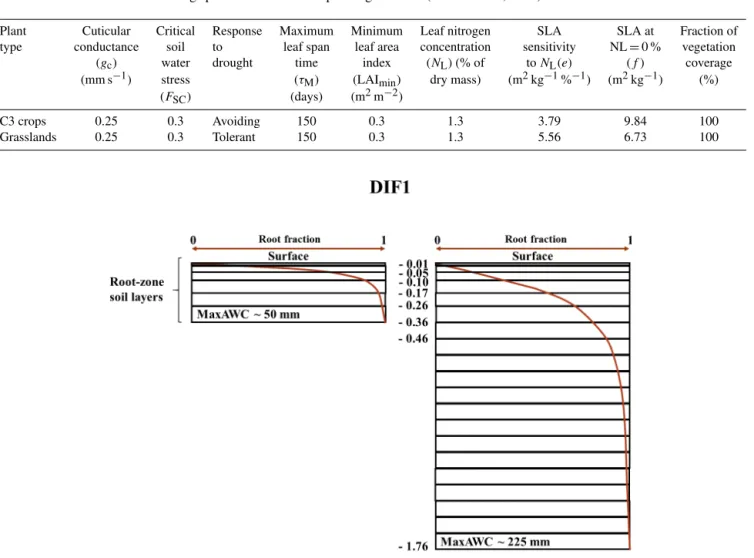
Table 1.Standard values of ISBA-A-gs parameters for C3 crops and grasslands (Gibelin et al., 2006).
Plant Cuticular Critical Response Maximum Minimum Leaf nitrogen SLA SLA at Fraction of type conductance soil to leaf span leaf area concentration sensitivity NL=0 % vegetation
(gc) water drought time index (NL) (% of toNL(e) (f) coverage (mm s−1) stress (τ
M) (LAImin) dry mass) (m2kg−1%−1) (m2kg−1) (%) (FSC) (days) (m2m−2)
C3 crops 0.25 0.3 Avoiding 150 0.3 1.3 3.79 9.84 100 Grasslands 0.25 0.3 Tolerant 150 0.3 1.3 5.56 6.73 100
Figure 4.Soil profile of the DIF1 experiment. The soil depth within the root zone is in metres. Only two configurations are represented: for the minimum (left panel) and maximum (right panel) values of MaxAWC (50 and 225 mm, respectively). The cumulative root density profile for crops (Eq. 1 withRe=0.961) is represented by a brown line. A top soil layer of 1 cm is represented.
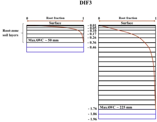
– DIF1 uses the new DIF capability of SURFEX v7.2 (Fig. 4). As in FR-2L, the root zone corresponds to the whole soil layer. The root profile reaches the bottom of the soil layer, and the total soil depth corresponds todR.
– DIF2 includes additional subroot-zone base flow soil layers with respect to DIF1, and the deep soil layers contribute to plant transpiration through capillary rises. It is assumed that MaxAWC is governed by the limited capacity of the plants to develop a root system in a deep soil, and the number of subroot-zone layers decreases when the rooting depth increases. A constant total soil depth of 1.96 m is prescribed, anddRis varied between
0.36 and 1.76 m (Fig. 5).
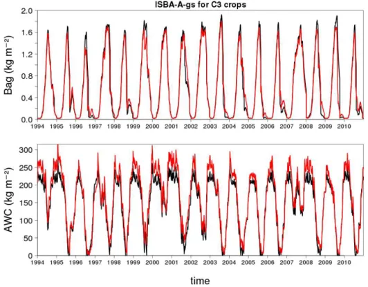
– DIF3 is similar to DIF1, as soil depth is the main limi-tation to root water extraction. However, two additional base flow soil layers contribute to transpiration through capillary rises. The total soil depth and dR are varied
simultaneously, and two adjacent 0.1 m thick deep soil layers are represented (Fig. 6).
– DIF1-NRT permits assessment of the impact of a re-fined representation of the CO2 uptake by the
vegeta-tion on theBaginter-annual variability, as the NRT light
absorption option is used together with DIF1.
– DIF1-Uniform permits assessment of the sensitivity of the ISBA-A-gs simulations to the shape of the root den-sity profile. It corresponds to DIF1 simulations using a uniform root density profile instead of Eq. (1). These simulations are performed over the 61-Orne départe-ment (see Sect. 4.1).
2.5 Atmospheric forcing
Figure 5.As in Fig. 4, except for the DIF2 experiment. Subroot soil layers are added (blue lines) down to a constant soil depth of 1.96 m.
des Renseignements Atmosphériques à la Neige”) mesoscale atmospheric analysis system (Durand et al., 1993, 1999). Pre-cipitation, air temperature, air humidity, wind speed, incom-ing solar radiation and incomincom-ing infra-red radiation are pro-vided over France at an 8 km×8 km spatial resolution on
an hourly basis. The SAFRAN product was evaluated by Quintana-Seguí et al. (2008) using independent in situ obser-vations. One-dimensional model simulations are performed at the 8 km×8 km spatial resolution of SAFRAN in grid
cells corresponding to cereal and natural grassland départe-ments (Fig. 1). These grid cells correspond to plots located within a département and with at least 45 % of their surface covered by either grasslands or crops, according to the aver-age plant functional type coveraver-age given by the 1 km×1 km
ECOCLIMAP-II global database (Faroux et al., 2013). 2.6 Optimisation of two key parameters
In this study, the method proposed by Ca12 is used: the val-ues of two key parameters of the ISBA-A-gs simulations, MaxAWC andgm, are explored, and the parameter pair
pro-viding the best correlation coefficient (r) of the maximum annual value ofBag(BagX) and GY (DMY) is selected, for
C3 crops (grasslands). For the FR-2L experiment, the opti-misation of both MaxAWC and gm is performed for all the
départements of Fig. 1. For the DIF1, DIF2, and DIF3 ex-periments, only MaxAWC is optimised, and the gm values
derived from the FR-2L optimisation are used. In the case of crops, simulatedBagvalues after 31 July are not considered,
in order to be consistent with the theoretical averaged harvest dates in France. Attempts were made to use other dates in July (not shown) without affecting the results of the analysis. On the other hand, new optimal gm values are obtained
to-gether with MaxAWC for the DIF1-NRT experiment, as the representation of photosynthesis at canopy level differs from that of the other experiments. Moreover, major differences with Ca12 are that (1) a longer period is considered (1994– 2010 instead of 1994–2008 in Ca12), and that (2) a more de-tailed screening of MaxAWC values is performed (12 values are considered, against 8 values in Ca12).
For all the experiments, MaxAWC ranges from 50 to 225 mm, with a lower increment between the small values (50, 62.5, 75, 87.5, 100, 112.5, 125, 137.5, 150, 175, 200 and 225 mm; 12 in total).
For thegmparameter, the same range of values as in Ca12
is used (from 0.50 to 1.75 mm s−1, six in total). For the three
simulations DIF1, DIF2 and DIF3, the same values of opti-mal gm obtained for each département and vegetation type
with the FR-2L version are used.
2.7 Metrics used to quantify the inter-annual variability In Sect. 4, the following metrics are used: the annual coeffi-cient of variation (ACV), computed as the ratio of the stan-dard deviation (σ) of the simulated BagX to the long-term
meanBagX,
ACV=σ BagX
/BagX, (7)
and the scaled anomaly (AS) ofBagXof a given year (yr)
AS,BagX(yr)=
BagX(yr)−BagX σ BagX
. (8)
This metric is also called thezscore, and can be applied to the Agreste cereal GY,
AS,GY(yr)=GY
(yr)−GY
σ (GY) , (9)
and to the Agreste grassland DMY, AS,DMY(yr)=DMY
(yr)−DMY
σ (DMY) . (10)
3 Results
3.1 Inter-annual variability ofBagX values
3.1.1 DIF1 vs. FR-2L
Figures 7 and 8 show an example of the inter-annual vari-ability of the simulatedBag and AWC (in kg m−2) as
sim-ulated by FR-2L and DIF1 for C3 crops and grasslands of the 61-Orne département. The optimal parameter values for C3 crops and grasslands are 1.75 and 0.5 mm s−1forg
m, and
200 and 50 mm for MaxAWC, respectively.
For C3 crops (Fig. 7),BagXvalues for FR-2L tend to reach
slightly higher values than for DIF1. The largest difference is observed in 1996. Furthermore, some differences occur in the senescence period, especially in 2001 and 2009. Conversely, the simulated AWC values are higher for DIF1, especially in winter. For both simulations, the wintertime AWC is of-ten higher than MaxAWC (set to 200 mm), in relation to wa-ter accumulation above field capacity, under wet conditions. This phenomenon is more pronounced for DIF1 than for FR-2L. Crop re-growth is simulated by both FR-2L and DIF1 during years with a marked summer drought, in 1995, 1996, 1998, 2006 and 2010. During wet years (i.e. in 1994, 2000 and 2007), the two experiments provide similar AWC values in summertime.
For grasslands (Fig. 8), the twoBag simulations are also
very close. However, contrary to C3 crops, theBag values
of the FR-2L simulation tend to be slightly lower than the DIF1 ones (e.g., in 1997, 2002, 2007, and 2009). The other difference with C3 crops is the systematic occurrence of regrowths.
3.1.2 ISBA-A-gs simulations vs. Agreste observations The départements where FR-2L BagX simulations present
Figure 7.Simulations over the 1994–2010 period for C3 crops (gm=1.75 mm s−1, MaxAWC=200 mm) in the 61-Orne département of (top
panel) the above-ground biomass and (bottom panel) the available water content in the root zone, using the FR-2L and DIF1 configurations (black and red lines, respectively).
Table 2.Median MaxAWC value and mediangmvalue under well-watered conditions, derived for each experiment (1) and number of
départements where the simulatedBagXpresents significant correlations (2) with the annual yields of Agreste statistics for six cereals (winter
wheat, rye, winter barley, spring barley, oat and triticale) and for permanent grasslands in France over the 1994–2010 period. Median values are in bold.
Plant type C3 crops Grasslands
Experiment FR-2L DIF1 DIF2 DIF3 DIF1-NRT FR-2L DIF1 DIF2 DIF3 DIF1-NRT
Median and 1.75 1.75 1.75 1.75 1.75 1.38 1.38 1.50 1.25 1.25
standard deviation 0.40 0.53 0.51 0.53 0.56 0.48 0.49 0.47 0.49 0.42 of optimalgm
(mm s−1)
Median and 125 112.5 81.3 93.8 100 81.3 68.8 75.0 75.0 75.0
standard deviation 54.0 61.3 84.0 63.0 64 55.0 54.0 55.0 58.0 58.0 of optimal
MaxAWC (mm)
Number of 45 48
départements
Number of 12–5 10–3 6–2 10–3 13–4 34–22 36–20 27–10 33–16 37–19 départements
presenting significant correlations (at 1 and 0.1 % levels)
1The optimisation ofgmis performed for FR-2L and DIF1-NRT only; DIF1, DIF2, and DIF3 use the same département-levelgmvalues as FR-2L.2Significant correlations at the 1 and 0.1 % levels correspond to coefficient of determination (R2) values higher than 0.366 and 0.525, respectively.
Figure 9.Best FR-2L simulation vs. Agreste statistical correlation levels obtained for (left panel) C3 crops and (right panel) grasslands. Non-significant, significant at the 1 % level, and significant at the 0.1 % level correlations are indicated in red squares, yellow dots and black dots, respectively.
and DMY time series are presented in Fig. 9, and the re-trievedgmand MaxAWC median values are presented in
Ta-ble 2 for all the experiments, together with the number of dé-partements presenting significant correlations with Agreste, for C3 crops and grasslands. With FR-2L, 12 (5) départe-ments present significant positive correlations at the 1 % (0.1 %) level for C3 crops. For grasslands, 34 (22) départe-ments present significant positive correlations at the 1 %
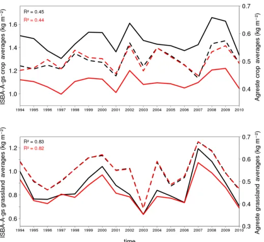
Figure 10. Averaged simulated yearlyBagX values (ISBA-A-gs, solid lines) and averaged observed agricultural yields (Agreste, dashed
lines) for départements with significant correlations (R2) at the 1 % level, with both FR-2L (black solid line) and DIF1-NRT (red solid line) simulations for (top panel) C3 crop GY and (bottom panel) grassland DMY.
against 6 (2) for DIF2. For the grasslands, a larger propor-tion of départements (among 48) presents significant corre-lations, from 27 (10) départements for DIF2 to 36 (20) for DIF1. The addition of deep soil layers below the root zone tends to degrade the results, especially in DIF2. Finally, the DIF1-NRT simulations perform as well as FR-2L or better, with 13 (4) and 37 (19) départements presenting significant positive correlations at the 1 % (0.1 %) level for C3 crops and grasslands, respectively.
Selecting the départements where the optimisation is suc-cessful, i.e. where the correlation betweenBagX and GY or
DMY is significant (p value<0.01), the time series of the mean BagX and mean GY and of the meanBagX and mean
DMY are compared in Fig. 10 for both the FR-2L and DIF1-NRT experiments. The inter-annual variability of the grass-land DMY is better represented byBagX than for the cereal
GY, with R2=0.83 and R2=0.45, respectively. The FR-2L experiment presents slightly betterR2values than DIF1-NRT. For C3 crops, it appears that the two experiments are not able to represent the lower GY in 2007, or the higher GY in 2004. For grasslands, the two experiments are not able to represent the lower DMY in 1996.
3.2 Impact of subroot-zone soil layers 3.2.1 Optimal MaxAWC values
Table 2 shows that, for C3 crops, the median MaxAWC value is higher for FR-2L than for DIF1 (125.0 and 112.5 mm, respectively). For DIF2 and DIF3, the median MaxAWC is even lower (81.3 and 93.8 mm, respectively). For grasslands, the median MaxAWC is less variable from one experiment to another (from 68.8 to 81.3 mm). In Table 2, the median Max-AWC values are calculated irrespective of which Agreste ce-real GY values are used to derive MaxAWC. Among the 10 départements with DIF1 simulations presenting signifi-cant correlations at the 1 % level with Agreste, 8 départe-ments share the same cereal Agreste yields as FR-2L.
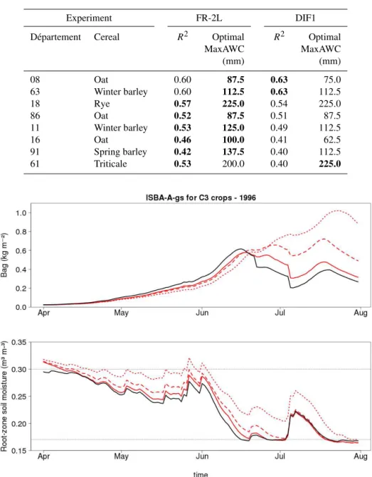
Table 3.Optimal MaxAWC and squared correlation coefficient (R2) betweenBagXand Agreste for FR-2L and DIF1 simulations at
départe-ments where the same cereal Agreste data are used and where the correlation betweenBagXvalues and the yields of Agreste statistics are
significant at least at the 1 % level. The highest MaxAWC andR2values at a given département are in bold.
Experiment FR-2L DIF1
Département Cereal R2 Optimal R2 Optimal
MaxAWC MaxAWC
(mm) (mm)
08 Oat 0.60 87.5 0.63 75.0
63 Winter barley 0.60 112.5 0.63 112.5
18 Rye 0.57 225.0 0.54 225.0
86 Oat 0.52 87.5 0.51 87.5
11 Winter barley 0.53 125.0 0.49 112.5
16 Oat 0.46 100.0 0.41 62.5
91 Spring barley 0.42 137.5 0.40 112.5
61 Triticale 0.53 200.0 0.40 225.0
Figure 11.Simulations in 1996 for C3 crops (gm=0.5 mm s−1, MaxAWC=75 mm) in the 08-Ardennes département of (top panel)
above-ground biomass and (bottom panel) root-zone soil moisture in the DIF1, DIF2, DIF3 and FR-2L configurations (red solid, red dotted, red dashed, and black lines, respectively). The grey lines indicate the root-zone soil moisture values at field capacity and at wilting point.
DIF1 root density profile tends to increase the impact of drought on plant growth for this département. Also, the largest difference inR2between FR-2L and DIF1 is observed for this département.
3.2.2 Plant growth
Table 2 shows that in DIF2 simulations the number of dé-partements with a significant correlation at the 1 % level is lower than in other experiments. The use of DIF2 has a
detri-mental impact on the representation of the inter-annual vari-ability by the plant growth model. Figure 11 shows the im-pact of the root water uptake model on the simulated C3 crop Bagand root-zone soil moisture for the 08-Ardennes
départe-ment during the growing season, from April to July 1996. In the FR-2L, DIF1, DIF2, and DIF3 simulations shown in Fig. 11, the samegm=0.5 mm s−1 and MaxAWC=75 mm
during the second half of July. At the same time, the DIF2 root-zone soil moisture presents the highest values. It appears that in the DIF2 simulation, the additional water supplied by capillary rises from the subroot-zone soil layers has a marked impact on the phenology, with the date of maximum Bag
shifted to the end of July and a much higherBagXvalue than
in the other experiments (1.02 kg m−2for DIF2, against 0.62, 0.58, and 0.72 kg m−2for FR-2L, DIF1, and DIF3, respec-tively). The same phenomenon happens in the DIF3 simula-tion to a lesser extent. In particular, the DIF3BagXis not very
different from the FR-2L one. The DIF1 simulation is closer to FR-2L. When the root-zone soil moisture reaches the wilt-ing point (equal to 0.17 m3m−3, as indicated in Fig. 11 by
the dashed line), the senescence starts. A marked water stress occurs and impacts photosynthesis and biomass production. Since water is supplied by the subroot-zone soil layers of DIF2 and DIF3, the wilting point is reached later than for FR-2L and DIF1, and the senescence starts later.
In FR-2L, the growth ofBagis faster than in the other
sim-ulations. This leads to a slightly higher value ofBagX than
for DIF1. This is related to the lower FR-2L root-zone soil moisture in May. In the drought-avoiding C3 crop parame-terisation of ISBA-A-gs, a moderate soil moisture stress trig-gers an increase in water use efficiency (Calvet, 2000) and enhances plant growth.
4 Discussion
4.1 Are the Jackson root profile model (Eq. 1) and the resulting water availability (Eq. 5) applicable on a regional scale?
In the DIF simulations, the stress function depends on the distribution of root density through Eqs. (5)–(6). This allows the lower layers to sustain the transpiration rate to some ex-tent when the upper soil layers dry out. However, one may emphasise that the approach used in this study to simulate the root water uptake is relatively simple, and may not be rele-vant to representing what really happens on a regional scale. Higher-level models are able to simulate the root network ar-chitecture and the three-dimensional soil water flow (Schnei-der et al., 2010; Jarvis, 2011). Also, the hydraulic redistri-bution of water from wetter to drier soil layers by the root system (hydraulic lift) is not simulated in this study. Siquiera et al. (2008) have investigated the impact of hydraulic lift us-ing a detailed numerical model, and showed that this effect could be significant.
Another difficulty in the implementation of DIF simula-tions is that the proposed Re values in Eq. (1) are the
re-sult of a meta-analysis. A single Revalue is proposed for a
given vegetation type, while large variability of Re can be
observed. This is particularly true for crops, and Fig. 1 in Jackson et al. (1996) shows thatY (dk)andRepresent much
higher variability for crops than for temperate grasslands.
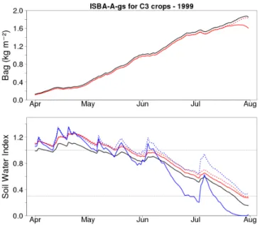
Figure 12.Simulations in 1999 for C3 crops (gm=1.75 mm s−1,
MaxAWC=225 mm, dR=1.76 m) in the 61-Orne department
of (top panel) above-ground biomass, and (bottom panel) SWITOP(dR) for FR-2L (black line), DIF1 (red solid line), and
DIF1-Uniform (red dotted line), and SWITOP (0.46 m) for DIF1 (blue solid line) and DIF1-Uniform (blue dotted line).
This difficulty may explain the shortcomings of DIF1 sim-ulations for the 61-Orne département described in Sect. 3.2.1 (Table 3). In particular, the root density in the top soil layers has a large impact on the water stress modelling.
This is demonstrated by performing an additional DIF1 simulation (DIF1-Uniform) using a uniform root density pro-file instead of Eq. (1). Figure 12 shows the evolution ofBag,
SWITOP(dR)and SWITOP(0.46 m) for the FR-2L, DIF1 and
DIF1-Uniform simulations for the 61-Orne département over the period from April to July 1999. For all the simulations, gm=1.75 mm s−1and MaxAWC=225 mm. TheBag
evolu-tion during the first 3 months is similar in the three simula-tions, with slightly faster growth for FR-2L. However, while senescence occurs in mid-July for DIF1, it occurs only at the end of July for FR-2L and DIF1-Uniform. Using the Jackson root density profile in Eq. (5) rather than a uniform profile has a marked impact on the simulated water balance. In situations where the top soil layers are drier (wetter) than deep soil lay-ers (i.e. present lower (higher)FSivalues), the totalFSvalue
is lower (higher) in DIF1 simulations than in FR-2L or DIF1-Uniform simulations. This tends to trigger an earlier senes-cence in DIF1 simulations. The early senessenes-cence for DIF1 is related to values of SWITOP getting close to zero at the top
fraction of the root zone: while SWITOP (0.46 m) decreases
simula-Figure 13. Simulations over the 1994–2010 period in the 61-Orne département of the above-ground biomass for (top panel) C3 crops (gm=1.75 mm s−1, MaxAWC=225 mm) and (bottom panel) grasslands (gm=0.50 mm s−1, MaxAWC=50 mm) for the DIF1 and
DIF1-NRT configurations (black and red lines, respectively).
tion. For C3 crops, a drought-avoiding response to soil water stress is simulated, triggering an increase in WUE (and in the plant growth rate) as soon asθis less thanθFC. Since the
DIF1 simulations tend to accumulate water above the field capacity (i.e. θ remains longer aboveθFC than for FR-2L),
the increase in WUE tends to occur later than for FR-2L. Fi-nally, theBagXvalue for FR-2L and DIF1-Uniform is higher
than for DIF1. This root profile effect also has an impact on the inter-annual variability and partly explains the lowerR2 value for DIF1 in Table 3 for this département.
Figure 12 shows that situations in which the top soil lay-ers are drier than deep soil laylay-ers tend to be more frequent in DIF1 simulations than in DIF1-Uniform simulations, in relation to the enhanced root water uptake close to the soil surface. Therefore, for given MaxAWC and soil wetness con-ditions, the totalFS values tend to be lower in DIF1
simula-tions than in DIF1-Uniform (and FR-2L) simulasimula-tions. This results in less evapotranspiration and less GPP. The lower GPP in DIF simulations results in lowerBagX values,
espe-cially for cereals as illustrated in Fig. 10. As noted by Feddes et al. (2001), the limitation of transpiration in DIF simula-tions when a great deal of water is still available at depth is probably too severe. In the real world, plants are able to transfer water uptake to compensate for water stress in the top layers, and DIF simulations cannot adequately account
for it. This fact probably explains part of why this model is not able to outperform the FR-2L simulations.
4.2 Do changes in the representation of
photosynthesis have an impact on the model performance?
In this section, the impact of the revised vegetation radia-tive transfer scheme and the refreshedgmparameter
(DIF1-NRT experiment) is discussed. Table 2 shows that while the DIF1-NRT results are close to those of DIF1 for grasslands, DIF1-NRT tends to outperform DIF1 for C3 crops. Figure 13 presents the simulatedBag of C3 crops and grasslands for
the DIF1 and DIF1-NRT simulations in the 61-Orne départe-ment over the 1994-2010 period. The two grassland simula-tions are very similar. On the other hand, the two C3 crop simulations differ inBagXvalues. The mean simulatedBagX
values for C3 crops are 1.61 and 1.32 kg m−2for DIF1 and
DIF1-NRT, respectively. The lowerBagXvalues simulated by
DIF1-NRT are related to the lowest gross primary production simulated by this version of the ISBA-A-gs model (Carrer et al., 2013). Also, DIF1-NRT simulates shorter growing peri-ods and a slightly enhanced inter-annual variability: the ACV (see Sect. 2.7) is equal to 7.4 % for DIF1, and to 8.4 % for DIF1-NRT. For grasslands, the mean simulatedBagX values
respec-Table 4.Correspondence between simulated and observed extreme years for départements with significant correlations (R2) at the 1 % level with both the FR-2L and DIF1-NRT simulations for C3 crops and grasslands as shown in Fig. 10. Favourable (unfavourable) years are defined aszscoresAS,BagXorAS,DMYhigher (lower) than 1.0 (−1.0). Years withAS,DMYhigher (lower) than 1.5 (−1.5) are in bold.
Favourable Unfavourable Normal (false)
Plant type Experiment True False True False While While favourable unfavourable
C3 crops FR-2L 2002, 2008, 2009 1997, 2010 2004 2001,2007
DIF1-NRT 2002, 2009 2008 2001 1997 1998, 2004 2003,2007
Grasslands FR-2L 2007, 2008 2000 2003, 2010 1996
DIF1-NRT 2000,2007, 2008 2003, 2010 1996
tively, and ACV values for DIF1 and DIF1-NRT are both equal to 30 %.
4.3 Can the ISBA-A-gs model predict the relative gain or loss of agricultural production during extreme years?
ISBA-A-gs is not a crop model, and does not predict yield per se. The background assumption of this work is that the regional-scale above-ground biomass simulated by a generic LSM can be used as a proxy for GY or DMY in terms of inter-annual variability. The quantitative consistency be-tween the simulated biomass and the agricultural statistics was discussed extensively by Ca12 (Sect. 3.3 and Figs. 12 and 13 in Ca12). For cereals, they considered the ratio of crop yield to the maximum above-ground biomass, called the har-vest index. The later ranged from 20 to 50 %, and this was consistent with typical harvest index values given by Bon-deau et al. (2007) for temperate cereals. The same result is obtained in this study (not shown). For grasslands, Ca12 sim-ulated both managed and unmanaged grasslands. For man-aged grasslands, DMY was explicitly simulated, and ranged from 0.1 to 0.8 kg m−2. The scatter of the simulated DMY
was relatively small, with a standard deviation of differences with the Agreste DMY of 0.20 kg m−2. ISBA-A-gs tended slightly to underestimate DMY values, with a mean bias of
−0.08 kg m−2. For unmanaged grasslands, the simulatedBag
was 0.17 kg m−2higher than the Agreste DMY values, on av-erage. In this study, unmanaged grasslands were considered, only, and results similar to those of Ca12 were found (not shown).
The ISBA-A-gs model is optimised to maximise the corre-lation coefficient between Agreste GY (or DMY) and mod-elledBagX. The resulting scores are used to assess the
capa-bility of a given model configuration to represent the inter-annual variability of BagX over the 1994–2010 period. In
studies where the objective of the model calibration is to im-prove the model prediction for operational applications, the model quality needs to be confirmed in an independent run with data not used during the calibration. An example of a rigorous calibration and validation procedure in hydrology
can be found in Refsgaard (1997). In this study, a valida-tion run was not performed, as the considered period was too short to apply a split-sample procedure and separate calibra-tion and validacalibra-tion sub-periods. Moreover, the objective of this study is to benchmark DIF options, not to predict the agricultural yields. Therefore, using an independent data set to assess yield prediction is not needed.
While the main objective of this work is to evaluate con-trasting root water uptake models using agricultural statistics, one can investigate how the resultingBagX values react to
extreme years (either favourable or unfavourable to agricul-tural production). The best simulations result from the op-timisation of the MaxAWC parameter. Table 4 summarises the true and false detection of favourable and unfavourable years. The latter are defined asAS,BagX or AS,DMY values higher (lower) than 1.0 (−1.0). TheAS,BagX orAS,DMY val-ues are based on the mean time series of Fig. 10. The un-detected favourable and unfavourable years are also listed in Table 4. The best detection performance is obtained by DIF1-NRT for grasslands, with only 1996 not detected as unfavourable. The worst detection performance is obtained by DIF1-NRT for C3 crops, with 2003 and 2007 not detected as unfavourable, 1998 and 2004 not detected as favourable, 1997 wrongly detected as unfavourable, and 2008 wrongly detected as favourable. For grasslands, the extreme years, defined as AS,DMY values higher (lower) than 1.5 (−1.5),
are 2007 (favourable) and 2003 (unfavourable). These two cases are correctly identified in the two experiments. For C3 crops, the most favourable years are 2002 and 2009, and the most unfavourable year is 2007. While 2002 and 2009 are correctly identified in the two experiments, 2007 is not detected. The higher performance in the representation of extreme years for grasslands than for C3 crops is consistent with the results of Table 2 showing that significant correla-tions betweenBagX and DMY are obtained more often than
betweenBagX and GY. This can be explained by the more
pronounced inter-annual variability of the grassland DMY, with ACV=30 % against ACV values less than 10 % for the
lower than for cereals (Table 2). Finally, ISBA-A-gs has no direct representation of agricultural practices and the cereal GY, and the consistency betweenBagX and GY relies on the
hypothesis that the harvest index (the ratio of GY toBagX)
does not vary much from one year to another on the consid-ered spatial scale. This issue is discussed in Ca12. For grass-lands, the simulated BagX is more directly representative of
DMY. This explains why a better agreement of the simula-tions is found with the grassland DMY than with the cereal GY (Tables 2 and 4).
4.4 Prospects for better constraining MaxAWC
Ca12 have shown that MaxAWC is the main driver of the inter-annual variability ofBagin the ISBA-A-gs model.
Rep-resenting the year-to-yearBagvariability in a dynamic
vege-tation model is a prerequisite for correctly representing sur-face fluxes on all temporal scales (from hourly to decadal). Table 2 shows that significant differences in the represen-tation of the Bag inter-annual variability are triggered by
switching from one model option to another. Also, for a given model option, the mediangmand MaxAWC values obtained
for cereals contrast from those obtained for grasslands. This is very valuable information for guiding the mapping of the model parameters in future studies. It must be noted that using the inter-annual variability of plant growth to assess LSM parameters is a rather new idea. For example, Rosero et al. (2010) and Gayler et al. (2014) performed an assessment of key parameters of the Noah LSM, including a version with a dynamic vegetation module, using a set of experimen-tal stations. However, they did not address the inter-annual variability of plant growth, as their simulations covered one vegetation cycle only. Such a short simulation period is not sufficient for constraining those model parameters which af-fect the inter-annual variability of plant growth (Kuppel et al., 2012).
In addition to the intrinsic limitations related to the use of a generic LSM unable to represent agricultural practices (see above), uncertainties are generated by the data sets used to force the LSM simulations. For example, the incoming ra-diation in the SAFRAN atmospheric analysis can be affected by seasonal biases (Szczypta et al., 2011; Carrer et al., 2012). Since phenology in ISBA-A-gs is driven by photosynthesis, biases in the incoming radiation can impact the date of the leaf onset. The impact of errors in the forcing data is proba-bly more acute for cereals than for grasslands in relation to a shorter growing period. More research is needed to assess the impact of using enhanced atmospheric reanalyses (Weedon et al., 2011; Oubeidillah et al., 2014) and proxies for annual agricultural statistics such as gridded maximum LAI values at a spatial resolution of 1 km×1 km derived from satellite
products (Baret et al., 2013).
Another difficulty is that the coarse spatial resolution of agricultural statistics prevents the use of local soil properties (Sect. 2.3). Models need to be tested on a local scale using
data from instrumented sites. For example, the DIF version of ISBA was tested on a local scale by Decharme et al. (2011) over a grassland site in south-western France. However, the soil and vegetation characteristics at a given site may dif-fer sharply from those at neighbouring sites. It is important to explore new ways of assessing and benchmarking model simulations on a regional scale. Remote-sensing products can be used to monitor terrestrial variables over large areas and to benchmark land surface models (Szczypta et al., 2014). At the same time, using in situ observations as much as possible is key, as remote-sensing products are affected by uncertain-ties. So far, the French annual agricultural yield data have been publicly available on a département scale only. In order to take advantage of the existing information on soil proper-ties, an option could be to use satellite-derived LAI products at a spatial resolution of 1 km×1 km in conjunction with soil
maps at the same spatial resolution (e.g. derived from the Harmonized World Soil Database, Nachtergaele et al., 2012). Since these products are now available on a global scale, the methodology explored in this study over metropolitan France could be extended to other regions.
The ISBA-A-gs model is intended to bridge the gap be-tween the terrestrial carbon cycle and the hydrological sim-ulations (e.g. river discharge). In previous works, the ISBA-A-gs model was coupled to hydrological models able to sim-ulate river discharge (e.g. Queguiner et al., 2011; Szczypta et al., 2012). While simulating vegetation requires a good description of the soil water stress, hydrological simulations are sensitive to changes in the representation of the surface water and energy fluxes. The latter are controlled to a large extent by vegetation. As suggested by Feddes et al. (2001) and Decharme et al. (2013), the obtained “effective root dis-tribution function” could be validated using river discharge observations by coupling the LSM to a hydrological model. We will investigate this possibility in future work. Note how-ever that the river discharge is often impacted by anthro-pogenic effects such as dams and irrigation. Such effects are not completely represented in large-scale hydrological mod-els (Hanasaki et al., 2006).
5 Conclusions
with the Agreste agricultural statistics, for given vegetation and photosynthesis parameters. The impact on the results of the representation of the vegetation was assessed using an-other representation of the light absorption by the canopy and using refreshed values of the gmphotosynthesis parameter.
TheBagXtime series based on the multi-layer model without
additional subroot-zone base flow soil layers presented cor-relations with the agricultural statistics similar to those ob-tained with FR-2L. On the other hand, adding subroot-zone base flow soil layers tended to degrade the correlations. Over-all, a better agreement of the simulations was found with the grassland DMY than with the cereal GY in relation to sev-eral factors, such as (1) the more pronounced inter-annual variability of the grassland DMY, (2) the more direct corre-spondence betweenBagX and DMY, and (3) less variability
Appendix A
Table A1.Nomenclature.
List of symbols
ACV Annual coefficient of variation (%) AS,BagX (yr) Scaled anomaly ofBagXof a given year (–)
AS,DMY(yr) Scaled anomaly of DMY of a given year (zscore) (–)
AS,GY(yr) Scaled anomaly of GY of a given year (zscore) (–)
AWC Simulated available soil water content (kg m−2)
Bag Simulated above-ground biomass (kg m−2)
BagX Maximum of simulated above-ground biomass (kg m−2)
DIF Multi-layer diffusion model
di Depth of a soil layer within the root zone (m) DMY Dry matter yields of grasslands (kg m−2) Dmax Maximum leaf-to-air saturation deficit (kg kg−1)
dR Root-zone depth (m)
FS Soil water stress function (–)
FSC Critical soil water stress (0.3 in this study)
FR-2L Two-layer force–restore model FT Plant transpiration flux (kg m−2s−1)
gm Mesophyll conductance in well-watered conditions (mm s−1)
GY Annual grain yields of crops (kg m−2)
LAI Leaf area index (m2m−2)
LSM Land surface model
MaxAWC Maximum available soil water content (kg m−2)
NIT Photosynthesis-driven plant growth version of ISBA-A-gs NL Leaf nitrogen concentration (% of leaf dry mass)
NRT New radiative transfer scheme within the vegetation PAR Photosynthetically active radiation (W m−2) Re Root extinction coefficient (–)
SLA Specific leaf area (m2kg−1) ST Root water uptake (kg m−2s−1) SWI Soil wetness index (–)
WUE Leaf-level water use efficiency (ratio of net assimilation of CO2to leaf transpiration)
Y Root density profile (–)
Greek symbols
ρ Water density (kg m−3)
θ Volumetric soil water content (m3m−3)
θFC Volumetric soil water content at field capacity (m3m−3)
θWILT Volumetric soil water content at wilting point (m3m−3)
The Supplement related to this article is available online at doi:10.5194/hess-11-4979-2014-supplement.
Acknowledgements. The doctoral scholarship of Nicolas Canal was funded by Agence Nationale de la Recherche Technique through a partnership between Météo-France and Arvalis-Institut du Végétal. S. Lafont was supported by the GEOLAND2 project, co-funded by the European Commission within the Copernicus initiative of FP7 under grant agreement no. 218795, and this study contributed to IMAGINES FP7 project no. 311766. The authors would like to thank Stéphanie Faroux for her help with the SURFEX simulations, as well as the three anonymous reviewers for their useful comments.
Edited by: N. Romano
References
Agreste: http://agreste.agriculture.gouv.fr/page-d-accueil/article/ donnees-en-ligne, last access: December 2014.
Agreste Bilans: Agreste Chiffres et Données Agriculture No. 209, Bilans d’approvisionnements agroalimentaires 2007–2008, 5 pp., http://agreste.agriculture.gouv.fr/IMG/file/aliments209. pdf (last access: December 2014), 2007.
Agreste Conjoncture: Bilan conjoncturel 2007, No: 10–11, 40 pp., http://agreste.agriculture.gouv.fr/IMG/pdf/bilan2007note.pdf (last access: December 2014), 2007.
Agreste Infos Rapides: Grandes cultures et fourrages, No. 7, Prairies, http://agreste.agriculture.gouv.fr/IMG/pdf/ prairie0711note.pdf (last access: December 2014), 2007. Baret, F., Weiss, M., Lacaze, R., Camacho, F., Makhmara, H.,
Pa-cholczyk, P., and Smets, B.: GEOV1: LAI and FAPAR essen-tial climate variables and FCOVER global time series capitaliz-ing over existcapitaliz-ing products, Part 1: Principles of development and production, Remote Sens. Environ., 137, 299–309, 2013. Bondeau, A., Smith, P. C., Zaehle, S., Schaphoff, S., Lucht, W.,
Cramer, W., Gerten, D., Lotze-Campen, H., Müller, C., Reich-stein, M., and Smith, B.: Modelling the role of agriculture for the 20th century global terrestrial carbon balance, Global Change Biol., 13, 679–706, 2007.
Boone, A., Masson, V., Meyers, T., and Noilhan, J.: The influ-ence of the inclusion of soil freezing on simulations by a Soil– Vegetation–Atmosphere Transfer Scheme, J. Appl. Meteorol., 39, 1544–1569, 2000.
Brisson, N., Gate, P., Gouache, D., Charmet, G., Oury, F.-X., and Huard, F.: Why are wheat yields stagnating in Europe? A com-prehensive data analysis for France, Field Crops Res., 119, 201– 212, doi:10.1016/j.fcr.2010.07.012, 2010.
Brut, A., Rüdiger, C., Lafont, S., Roujean, J.-L., Calvet, J.-C., Jar-lan, L., Gibelin, A.-L., Albergel, C., Le Moigne, P., Soussana, J.-F., Klumpp, K., Guyon, D., Wigneron, J.-P., and Ceschia, E.: Modelling LAI at a regional scale with ISBA-A-gs: compari-son with satellite-derived LAI over southwestern France, Bio-geosciences, 6, 1389–1404, doi:10.5194/bg-6-1389-2009, 2009. Calvet, J.-C.: Investigating soil and atmospheric plant water stress using physiological and micrometeorological data, Agr. Forest Meteorol., 103, 229–247, 2000.
Calvet, J.-C. and Soussana, J.-F.: Modelling CO2-enrichment ef-fects using an interactive vegetation SVAT scheme, Agr. Forest Meteorol., 108, 129–152, 2001.
Calvet, J.-C., Noilhan, J., Roujean, J., Bessemoulin, P., Ca-belguenne, M., Olioso, A., and Wigneron, J.: An interactive veg-etation SVAT model tested against data from six contrasting sites, Agr. Forest Meteorol., 92, 73–95, 1998.
Calvet, J.-C., Gibelin, A.-L., Roujean, J.-L., Martin, E., Le Moigne, P., Douville, H., and Noilhan, J.: Past and future scenarios of the effect of carbon dioxide on plant growth and transpiration for three vegetation types of southwestern France, Atmos. Chem. Phys., 8, 397–406, doi:10.5194/acp-8-397-2008, 2008.
Calvet, J.-C., Lafont, S., Cloppet, E., Souverain, F., Badeau, V., and Le Bas, C.: Use of agricultural statistics to verify the interannual variability in land surface models: a case study over France with ISBA-A-gs, Geosci. Model Dev., 5, 37–54, doi:10.5194/gmd-5-37-2012, 2012.
Calvet, C., Rivalland, V., Picon-Cochard, C., and Guehl, J.-M.: Modelling forest transpiration and CO2 fluxes – response to soil moisture stress, Agr. Forest Meteorol., 124, 143–156, doi:10.1016/j.agrformet.2004.01.007, 2004.
Carrer, D., Lafont, S., Roujean, J. L., Calvet, J. C., Meurey, C., Le Moigne, P., and Trigo, I. F.: Incoming solar and infrared radiation derived from METEOSAT: Impact on the modelled land water and energy budget over France, J. Hydrometeorol., 13, 504–520, doi:10.1175/JHM-D-11-059.1, 2012.
Carrer, D., Roujean, J.-L., Lafont, S., Calvet, J.-C., Boone, A., Decharme, B., Delire, C., and Gastellu-Etchegorry, J.-P.: A canopy radiative transfer scheme with explicit FAPAR for the in-teractive vegetation model ISBA-A-gs: impact on carbon fluxes, J. Geophys. Res.-Biogeo., 118, 1–16, doi:10.1002/jgrg.20070, 2013.
Deardorff, J. W.: A parameterization of ground-surface moisture content for use in atmospheric prediction models, J. Appl. Mete-orol., 16, 1182–1185, 1977.
Deardorff, J. W.: Efficient prediction of ground surface temperature and moisture, with inclusion of a layer of vegetation, J. Geophys. Res., 20, 1889–1903, 1978.
Decharme, B., Boone, A., Delire, C., and Noilhan, J.: Local evalu-ation of the Interaction between Soil Biosphere Atmosphere soil multilayer diffusion scheme using four pedotransfer functions, J. Geophys. Res., 116, D20126, doi:10.1029/2011JD016002, 2011. Decharme, B., Martin, E., and Faroux, S.: Reconciling soil thermal and hydrological lower boundary conditions in land surface models, J. Geophys. Res.-Atmos., 118, 7819–7834, doi:10.1002/jgrd.50631, 2013.
de Rosnay, P., Calvet, J.-C., Kerr, Y., Wigneron, J.-P., Lemaître, F., Escorihuela, M. J., Sabater, J. M., Saleh, K., Barrié, J., Bouhours, G., Coret, L., Cherel, G., Dedieu, G., Durbe, R., Fritz, N. E. D., Froissard, F., Hoedjes, J., Kruszewski, A., Lavenu, F., Suquia, D., and Waldteufel, P.: SMOSREX: A long term field campaign experiment for soil moisture and land surface pro-cesses remote sensing, Remote Sens. Environ., 102, 377–389, doi:10.1016/j.rse.2006.02.021, 2006.
Durand, Y., Giraud, G., Brun, E., Merindol, L., and Martin, E.: A computer-based system simulating snow-pack structures as a tool for regional avalanche forecasting, Ann. Glaciol., 45, 469–484, 1999.
Faroux, S., Kaptué Tchuenté, A. T., Roujean, J.-L., Masson, V., Martin, E., and Le Moigne, P.: ECOCLIMAP-II/Europe: a twofold database of ecosystems and surface parameters at 1 km resolution based on satellite information for use in land surface, meteorological and climate models, Geosci. Model Dev., 6, 563– 582, doi:10.5194/gmd-6-563-2013, 2013.
Feddes, R. A., Hoff, H., Bruen, M., Dawson, T., de Rosnay, P., Dirmeyer, P., Jackson, R. B., Kabat, P., Kleidon, A., Lilly, A., and Pitman, A. J.: Modeling root water uptake in hydrological and climate models, B. Am. Meteorol. Soc., 82, 2797–2809, 2001. Gate, P., Brisson, N., and Gouache, D.: Les causes du
plafon-nement du rendement du blé en France: d’abord une origine cli-matique, Evolution des rendements des plantes de grande culture, Académie d’Agriculture de France, 5 May 2010, Paris, 9 pp., 2010.
Gayler, S., Wöhling, T., Grzeschik, M., Ingwersen, J., Wize-mann, H.-D., Warrach-Sagi, K., Högy, P., Attinger, S., Streck, T., and Wulfmeyer, V.: Incorporating dynamic root growth en-hances the performance of Noah-MP at two contrasting win-ter wheat field sites, Wawin-ter Resour. Res., 50, 1337–1356, doi:10.1002/2013wr014634, 2014.
Gibelin, A.-L., Calvet, J.-C., Roujean, J.-L., Jarlan, L., and Los, S. O.: Ability of the land surface model ISBA-A-gs to simulate leaf area index at the global scale: Compari-son with satellites products, J. Geophys. Res., 111, D18102, doi:10.1029/2005JD006691, 2006.
Hanasaki, N., Kanae, S., and Oki, T.: A reservoir operation scheme for global river routing models, J. Hydrol., 327, 22–41, 2006. Jackson, R. B., Canadell, J., Ehleringer, J. R., Mooney, H. A.,
Sala, O. E., and Schulze, E. D.: A global analysis of root distributions for terrestrial biomes, Oecologia, 108, 389–411, doi:10.1007/BF00333714, 1996.
Jacobs, C. M. J.: Direct impact of atmospheric C02enrichment on
regional transpiration, PhD thesis, Agricultural University, Wa-geningen, 179 pp., 1994.
Jacobs, C. M. J., van den Hurk, B. J. J. M., and De Bruin, H. A. R.: Stomatal behaviour and photosynthetic rate of unstressed grapevines in semi-arid conditions, Agr. Forest Meteorol., 80, 111–134, 1996.
Jarvis, N. J.: Simple physics-based models of compensatory plant water uptake: concepts and eco-hydrological consequences, Hy-drol. Earth Syst. Sci., 15, 3431–3446, doi:10.5194/hess-15-3431-2011, 2011.
Jarvis, P. G.: The interpretation of the variations in leaf wa-ter potential and stomatal conductance found in canopy in the field, Philos. T. Roy. Soc. Lond. B, 273, 593–610, doi:10.1098/rstb.1976.0035, 1976.
Krinner, G., Viovy, N., de Noblet-Ducoudré, N., Ogée, J., Polcher, J., Friedlingstein, P., Ciais, P., Sitch, S., and Prentice, I. C.: A dynamic global vegetation model for studies of the cou-pled atmosphere-biosphere system, Global Biogeochem. Cy., 19, GB1015, doi:10.1029/2003GB002199, 2005.
Kuppel, S., Peylin, P., Chevallier, F., Bacour, C., Maignan, F., and Richardson, A. D.: Constraining a global ecosystem model with
multi-site eddy-covariance data, Biogeosciences, 9, 3757–3776, doi:10.5194/bg-9-3757-2012, 2012.
Lafont, S., Zhao, Y., Calvet, J.-C., Peylin, P., Ciais, P., Maignan, F., and Weiss, M.: Modelling LAI, surface water and carbon fluxes at high-resolution over France: comparison of ISBA-A-gs and ORCHIDEE, Biogeosciences, 9, 439–456, doi:10.5194/bg-9-439-2012, 2012.
Masson, V., Le Moigne, P., Martin, E., Faroux, S., Alias, A., Alkama, R., Belamari, S., Barbu, A., Boone, A., Bouyssel, F., Brousseau, P., Brun, E., Calvet, J.-C., Carrer, D., Decharme, B., Delire, C., Donier, S., Essaouini, K., Gibelin, A.-L., Giordani, H., Habets, F., Jidane, M., Kerdraon, G., Kourzeneva, E., Lafaysse, M., Lafont, S., Lebeaupin Brossier, C., Lemonsu, A., Mahfouf, J.-F., Marguinaud, P., Mokhtari, M., Morin, S., Pigeon, G., Sal-gado, R., Seity, Y., Taillefer, F., Tanguy, G., Tulet, P., Vincendon, B., Vionnet, V., and Voldoire, A.: The SURFEXv7.2 land and ocean surface platform for coupled or offline simulation of earth surface variables and fluxes, Geosci. Model Dev., 6, 929–960, doi:10.5194/gmd-6-929-2013, 2013.
Nachtergaele, F., van Velthuize, H., Verelst, L., Wiberg, D., Batjes, N., Dijkshoorn, K., van Engelen, V., Fischer, G., Jones, A., Montanarella, L., Petri, M., Prieler, S., Teixeira, E., and Shi, X.: Harmonized World Soil Database (version 1.2), 2012, available at: http://webarchive.iiasa.ac.at/Research/LUC/ External-World-soil-database/HWSD_Documentation.pdf (last access: December 2014), 2012.
Noilhan, J. and Mahfouf, J.-F.: The ISBA land surface parameteri-sation scheme, Global Planet. Change, 13, 145–159, 1996. Noilhan, J. and Planton, S.: A simple parameterization of land
sur-face processes for meteorological models, Mon. Weather Rev., 117, 536–549, 1989.
Oubeidillah, A. A., Kao, S.-C., Ashfaq, M., Naz, B. S., and Tootle, G.: A large-scale, high-resolution hydrological model parameter data set for climate change impact assessment for the contermi-nous US, Hydrol. Earth Syst. Sci., 18, 67–84, doi:10.5194/hess-18-67-2014, 2014.
Queguiner, S., Martin, E., Lafont, S., Calvet, J.-C., Faroux, S., and Quintana-Seguí, P.: Impact of the use of a CO2responsive
land surface model in simulating the effect of climate change on the hydrology of French Mediterranean basins, Nat. Hazards Earth Syst. Sci., 11, 2803–2816, doi:10.5194/nhess-11-2803-2011, 2011.
Quintana-Seguí, P., Le Moigne, P., Durand, Y., Martin, E., Habets, F., Baillon, M., Canellas, C., Franchisteguy, L., and Morel, S.: Analysis of Near-Surface Atmospheric Variables: Validation of the SAFRAN Analysis over France, J. Appl. Meteorol. Clim., 47, 92–107, doi:10.1175/2007JAMC1636.1, 2008.
Refsgaard, J. C.: Parameterisation, calibration and validation of dis-tributed hydrological models, J. Hydrol., 198, 69–97, 1997. Rivalland, V., Calvet, J.-Ch., Berbigier, P., Brunet, Y., and Granier,
A.: Transpiration and CO2 fluxes of a pine forest: mod-elling the undergrowth effect, Ann. Geophys., 23, 291–304, doi:10.5194/angeo-23-291-2005, 2005.
Sabater, J. M., Jarlan, L., Calvet, J.-C., Bouyssel, F., and De Ros-nay, P.: From near-surface to root-zone soil moisture using dif-ferent assimilation techniques, J. Hydrometeorol., 8, 194–206, doi:10.1175/JHM571.1, 2007.
Schneider, C. L., Attinger, S., Delfs, J.-O., and Hildebrandt, A.: Im-plementing small scale processes at the soil-plant interface – the role of root architectures for calculating root water uptake pro-files, Hydrol. Earth Syst. Sci., 14, 279–289, doi:10.5194/hess-14-279-2010, 2010.
Seneviratne, S. I., Corti, T., Davin, E. L., Hirschi, M., Jaeger, E. B., Lehner, I., Orlowsky, B., and Teuling, A. J.: Investigating soil moisture-climate interactions in a changing climate: A review, Earth-Sci. Rev., 99, 125–161, doi:10.1016/j.earscirev.2010.02.004, 2010.
Siqueira, M., Katul, G., and Porporato, A.: Onset of water stress, hysteresis in plant conductance, and hydraulic lift: Scaling soil water dynamics from millimeters to meters, Water Resour. Res., 44, W01432, doi:10.1029/2007WR006094, 2008.
Smith, P. C., De Noblet-Ducoudré, N., Ciais, P., Peylin, P., Viovy, N., Meurdesoif, Y., and Bondeau, A.: European-wide simula-tions of croplands using an improved terrestrial biosphere model: Phenology and productivity, J. Geophys. Res., 115, G01014, doi:10.1029/2008JG000800, 2010a.
Smith, P. C., Ciais, P., Peylin, P., De Noblet-Ducoudré, N., Viovy, N., Meurdesoif, Y., and Bondeau, A.: European-wide simulations of croplands using an improved terrestrial biosphere model: 2. In-terannual yields and anomalous CO2fluxes in 2003, J. Geophys.
Res., 115, G04028, doi:10.1029/2009JG001041, 2010b.
Szczypta, C.: Hydrologie spatiale pour le suivi des sécheresses du bassin méditerranéen, INP Toulouse, 181 pp., 2012.
Szczypta, C., Calvet, J.-C., Albergel, C., Balsamo, G., Boussetta, S., Carrer, D., Lafont, S., and Meurey, C.: Verification of the new ECMWF ERA-Interim reanalysis over France, Hydrol. Earth Syst. Sci., 15, 647–666, doi:10.5194/hess-15-647-2011, 2011. Szczypta, C., Decharme, B., Carrer, D., Calvet, J.-C., Lafont, S.,
Somot, S., Faroux, S., and Martin, E.: Impact of precipitation and land biophysical variables on the simulated discharge of Eu-ropean and Mediterranean rivers, Hydrol. Earth Syst. Sci., 16, 3351–3370, doi:10.5194/hess-16-3351-2012, 2012.
Szczypta, C., Calvet, J.-C., Maignan, F., Dorigo, W., Baret, F., and Ciais, P.: Suitability of modelled and remotely sensed essential climate variables for monitoring Euro-Mediterranean droughts, Geosci. Model Dev., 7, 931–946, doi:10.5194/gmd-7-931-2014, 2014.