www.j-sens-sens-syst.net/5/381/2016/ doi:10.5194/jsss-5-381-2016
© Author(s) 2016. CC Attribution 3.0 License.
Optimization of a sensor for a Tian–Calvet calorimeter
with LTCC-based sensor discs
Franz Schubert1, Michael Gollner2, Jaroslaw Kita1, Florian Linseis2, and Ralf Moos1
1University of Bayreuth, Department of Functional Materials, 95440 Bayreuth, Germany 2LINSEIS Messgeräte GmbH, 95100 Selb, Germany
Correspondence to:Franz Schubert ([email protected])
Received: 4 August 2016 – Revised: 14 October 2016 – Accepted: 24 October 2016 – Published: 8 November 2016
Abstract. In this work, it is shown how a finite element method (FEM) model of a Tian–Calvet calorimeter is used to find improvements in the sensor design to increase the sensitivity of the calorimeter. By changing the layout of the basic part of the sensor, which is a low temperature co-fired ceramics (LTCC) based sensor disc, an improvement by a factor of 3 was achieved. The model was validated and the sensors were calibrated with a set of measurements that were later used to determine the melting enthalpies and melting temperatures of indium and tin samples. Melting temperatures showed a maximum deviation of 0.2 K while the enthalpy was measured with a precision better than 1 % for most samples. The values for tin deviate by less than 2 % from literature data.
1 Introduction
This work is conducted in the field of calorimetry, which is a state-of-the-art method of quantifying emission or adsorption of heat during physical or chemical processes (Höhne et al., 2003). A typical device is the calorimeter of the Tian–Calvet type. It has a cylindrical-type setup, meaning the cuvettes for both sample and reference are encompassed by a large num-ber of thermocouples to detect changes in the temperature difference between a sample and reference cuvette (Auroux, 2013; Calvet and Prat, 1963). A calibration run then deliv-ers a function between the measured temperature difference and the heat flow (Sarge et al., 1994). In our previous work, we have demonstrated the feasibility of a sensor for a Tian– Calvet calorimeter based on low temperature co-fired ce-ramics (LTCC) technology (Schubert et al., 2016). The base material for this process are green (unfired) glass-ceramics sheets that can be handled like plastic foils. The special fea-ture of this technique is the possibility of screen-printing functional pastes onto the unfired tapes and laminating lay-ers of tapes together by application of heat (70◦C) and pres-sure (21 MPa) (Kita et al., 2005). During firing, the polymers are being burned out and dense, mechanically stable ceram-ics with incorporated functional elements are achieved. For
further details please refer to Gongora-Rubio et al. (2001), Imanaka (2005) and Kita and Moos (2008), Kita et al. (2005). Using this process, a sensor1for a Tian–Calvet calorime-ter was developed using finite-element supported design. The main component of the sensor is a planar disc (in the follow-ing denoted as “sensor disc”), made of an LTCC rfollow-ing with a large number of thermocouples around the center that form a thermopile. A three dimensional sensor consists of several stacked sensor discs with a thermally isolating material in be-tween them. For this purpose, a porous aluminosilicate ma-terial that is commercially available to isolate high tempera-ture furnaces thermally was used. It has a very low thermal conductivity of about 0.1 W m−1K−1. As these porous fibers are very brittle, a simple and mechanically stable ring-shaped geometry was selected. All sensor discs are connected in se-ries. In our previous work, the sensitivity of the sensor was measured at room temperature using a heated cuvette that distributes the heat for calibration evenly amongst the sen-sor. To fully understand the scope of this work, the reader is referred to the previous paper by Schubert et al. (2016).
1The term “sensors”, as it is used in the calorimetry community,
Based on this proof of concept, the next steps to improve the sensor were conducted. A first step to improve the sen-sor was to understand how different design modifications af-fect the sensor performance. For this purpose, measurements with the existing design of the sensor discs were conducted at different temperatures to obtain data to validate the model. The model itself was much more comprehensive than in the previous work, e.g., the real geometry data of the existing sensor disc were included. After finding an optimized sen-sor design, an entire calorimeter was built, calibration mea-surements were conducted, and tin and indium samples were measured.
2 Optimization by finite-element method
2.1 Measurement setup and modeling
For the measurements, two sensors were mounted into an isothermal copper-block and connected in a differential setup by connecting the negative poles of each sensor and measur-ing the voltage between the positive poles of both sensors. Therefore, offset signals from sample and reference during heating cancel each other out. The device was heated by a heater coil around the copper block. The heater was closed-loop controlled to a Pt100 resistive temperature sensor that was positioned at the outer surface of the block. It is assumed that this position makes it easier to counteract temperature fluctuation resulting from changes in ambient temperature than if the sensor is positioned within the block, as the fluctu-ations can be counteracted before they reach the sensors. For further suppression of ambient temperature fluctuation, the whole device was covered with thermally isolating material. For calibration and test runs, the previously described metal and LTCC cuvettes were used (Schubert et al., 2016). For calibration, the internal heaters of the cuvettes were heated by a controlled current to release the defined power P. During melting experiments, the LTCC cuvettes with an inserted bottom in the middle were used. The whole setup is shown in Fig. 1.
In the original layout, 8 discs were used. In order to in-vestigate the influence of the number of sensor discs in the sensor and in order to get more parameters to validate the model, sensors with 16 sensor discs were built.
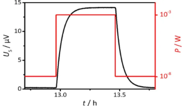
An exemplary measurement run to determine the sensi-tivity of a sensor with 16 sensor discs is shown in Fig. 2. During the experiment, a power of 1×10⁻⁸W was applied to establish a baseline before and after the calibration with 1×10⁻³W. Each power step was applied for 30 min. The thermovoltages were logged by a Keithley 2182A nanovolt-meter with a sampling rate of 0.5 Hz. The power P was applied in a pulse-like shape and the sensor voltage US re-sponds as shown in the typical plot in Fig. 2. The sensitivity was obtained by dividing the stationary value of signal
in-Figure 1.Setup of the Tian–Calvet device. It consists of a heated and isolated isothermal copper block with two sensors for sample and reference. The LTCC cuvettes have an integrated Pt500 resis-tance thermometer for calibration and temperature measurement.
Figure 2.Sensor responseUS at room temperature when the
ap-plied power to the testing cuvetteP is varied in a step-like pattern.
crease during heating1USbyP, as expressed in Eq. (1):
s=1US/P (1)
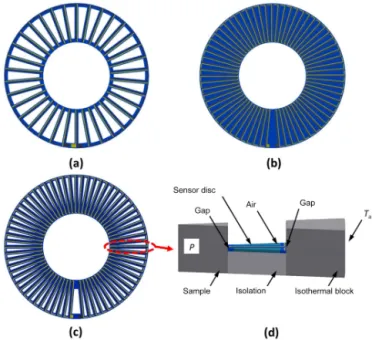
(Fig. 3c). Furthermore, an investigation was conducted into how doubling the number of thermocouples affects the sen-sor voltageUSby taking the original sensor disc and applying thermocouples on each side (top side and reverse side). Both the external diameter of 37 mm and the internal diameter of 17 mm as well as the thickness of about 0.53 mm remained constant.
In the course of the work, it became obvious that a precise model for the sensor has to consider not only the sensor discs, but also the isolation material as it contributes to the thermal conduction in the sensor. The radial and translational sym-metry of the sensor makes it possible to simplify the model and save computing resources by calculating the results for a slice with only one thermal leg. Figure 3d sketches the setup for the model, which also includes the gaps that occurred due to the tolerances of the sintered ceramics, which are in the order of 200 µm. For the isothermal block, the material was set to copper, and for the sample, a fictional material with a high thermal conductivity was used to ensure a uniform temperature distribution. In the studies, it was assumed that the sample releases a uniformly distributed power of 1 mW in the whole cuvette. As the model displays only a fraction of the real cuvette and sensor, only the appropriate volume share of total power was applied to the sample in the simula-tion. The temperature of the furnace was kept constant at the outer boundary of the model. The resulting sensitivityswas calculated according to Eq. (1) as the quotient of the total signal height1Usby the applied powerP. The results were corrected for the heat losses through top and bottom of the sensors that decrease the sensitivity by about 10 %, depend-ing on the sensor configuration.
2.2 Results of the modeling and first measurements
In Fig. 4a, the results of simulation and measurements for the original sensor disc are compared. Both model and sim-ulation show a sensitivity increase when the number of sen-sor discs is increased. The effect, however, is nonlinear and shows a kind of saturation for higher numbers of sensor discs, because of the higher thermal conductivity of the LTCC com-pared to the used isolation material. Therefore, the thermal conduction through the sensor increases with the number of sensor discs.
Figure 4a shows that the sensitivity increases with tem-perature for all sensor disc numbers. For 8 discs, the in-crease from 20 to 200◦C amounts to 63 %. This effect can be mainly attributed to the increasing Seebeck coefficient of the gold–platinum thermocouples, which increases by 75 % in this temperature range (Gotoh et al., 1991). The remaining difference is a result of the higher thermal conductivity of the used isolation materials at higher temperatures. The com-parison of simulation and measurement data obtained from stacks with 8 and 16 sensor discs shows a good agreement. The deviation at each temperature is less than 10 %.
Consid-Figure 3.Modeling was conducted on sensor discs with the original 34 thermocouples with cutouts(a), an increased number of 67 ther-mocouples without(b)and with cutouts(c). Additionally, a sensor disc with a design like(a), but with thermocouples printed on both sides, was tested in the model(d).
ering that some lesser-known material data had to be used for the simulations, this is a good result.
The good agreement between simulation and measure-ment allows for using the finite elemeasure-ment simulations to fur-ther develop the sensor. In the following Fig. 4b–d, model-ing results and obtained improvements for different designs are shown. For better comparability, the sensitivity of differ-ent sensor discs at 400◦C was plotted into a single diagram (Fig. 4e). The model-derived data are compared with the final device at the end of the paper. These data prove the validity of the model.
Increasing the number of thermocouples to 67, as shown in Fig. 4b, neither affects the shape of the curves, nor the sensitivity values largely. The voltageUS of the disc in re-lation to temperature rise of the sample will increase. At the same time, the thermal conduction from the sample to the furnace also increases as there is more material in radial di-rection to dissipate the heat. Thus, the released power of the sample causes less of a temperature increase. The effects of increased sensitivity for temperature and decreased tempera-ture increase neutralize each other almost completely which leads to a marginal increase in sensitivity.
The insertion of cutouts into the sensor disc decreases the thermal conductance and increases the sensitivity by 16 % at 20◦C for the stack with 8 discs. This effect would be smaller for a real part as the cutouts had to be rounded for manufac-turability.
sub-Figure 4.Sensitivitysfor sensors with different numbers of sensor discs (nsensor disc) in the stack and different designs of the sensor discs.
strates and the two thermopiles are connected in series by a single via. Figure 4c shows the sensitivity increase of this structure by more than 85 % for all temperatures and all num-ber of sensor discs. This is because the thermocouples are re-sponsible for less than 10 % of the heat flow from the center of the sensor to the circumference of the sensor. Doubling the number of thermocouples thereby doubles the generated voltageUSbut increases thermal losses only to some extent. Varying model parameters and geometry of the setup led to a deeper understanding of the system, and it was found that the gaps between the sensor and the isothermal block (due to manufacturing tolerances) have a detrimental effect on the sensor as they can be considered as thermal resistors that are connected in series with the sensor discs. Thus, the temper-ature gradient over the sensor disc decreases. By improving
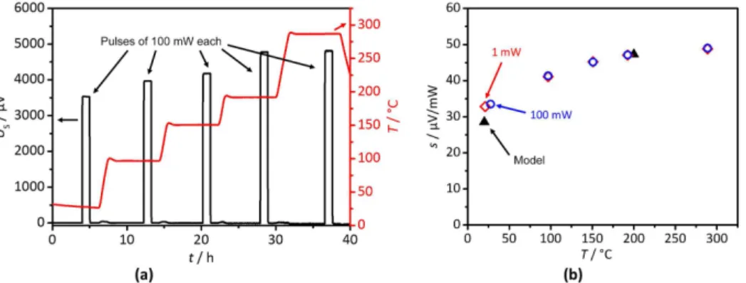
Figure 5.Sensor responseUSto different heating peaks of about 100 mW at different temperaturesT.(a)measurement(b)sensitivitysof
the system vs. temperatureT for model and measurement.
increased by a factor of about 3 compared to the original sen-sor as reported in Schubert et al. (2016) and as can be seen when comparing the sensitivities in Fig. 4e (“original 34” vs. the other curves).
The newly designed sensors were tested with LTCC cu-vettes at room temperature, 100, 200, and 300◦C, with an applied baseline power of 1×10⁻⁸W. Two calibration runs were made with either 100 or 1 mW. The sensor was heated to the different temperature plateaus with a rate of 1 K min−1 with a pause between the steps to ensure thermal equilibrium in the isothermal block before each measurement started. The sensor response US to the power pulses of 100 mW is depicted in Fig. 5a. The experiment has been conducted twice with a deviation of less than 1 %. All peaks show a good signal-to-noise ratio at all temperatures. For example, at 300◦C the signal height is1U
s=4830 µV, while the root mean square noise of the sensor signal is Us,rms=6.6 µV, which is a signal-to-noise ratio of SNR≈730.
The small shift in baseline that can be observed during heating between measurements is due the relatively high heating rate of 1 K min−1for this device and may stem from small asymmetries of the heater for the isothermal block. The sensor response US increases with temperature, which is a result of the increasing the Seebeck coefficient, start-ing with 33 µV mW−1 at room temperature and reaching 49 µV mW−1 at 300◦C. When comparing the sensitivity at 1 mW to the sensitivity at 100 mW it is noticed that both are identical (Fig. 5b), which means the system behaves linearly to applied power steps with no correction factor being nec-essary in this respect. The model fits to the measurements better than 1 % at 200◦C and about 15 % at room tempera-ture. The anomaly of high-temperature data fitting better than room temperature data is owing to the fact that data for ther-mal conductivity of the high temperature isolation material had to be extrapolated to room temperature as they were only available for high temperature.
From these measurements, the dependence of the sensitiv-ityson sample temperatureTcan be derived. This is called the calibration curve of the entire calorimeter. During
mea-surements of unknown substances, the sensor voltageUS is logged vs. timet. The sample temperatureTis logged, too. The time-dependent heat flow8is then obtained according to Eq. (2).
φ(t)=Us(t)
s(T) (2)
3 Measurements of real substances
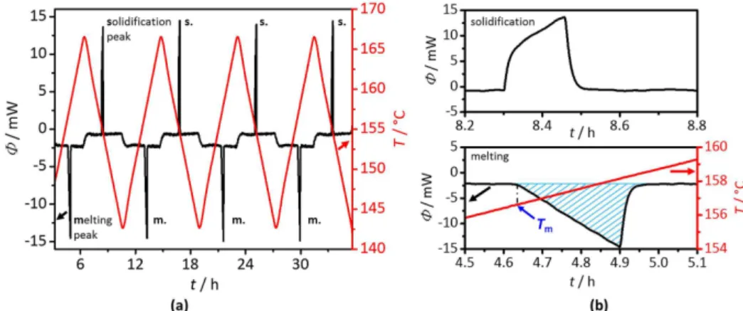
As a final test, real substances were used to see how the in-strument would perform for real samples when determining their melting temperatures and melting enthalpies. LTCC cu-vettes as shown in Fig. 1 were used with the sample, which was placed in the middle of the height of the cuvette. Samples of 0.0251 and 0.2149 g indium (In) and 0.0259 and 0.2136 g tin (Sn) were measured. To ensure thermal equilibrium of the sensor, the heating rate (β) during the experiments was 0.1 K min−1within a temperature of 10 K below and above the expected melting temperature. The temperature of the sample was logged with the internal Pt500 resistor of the cuvette, which is the closest possible point to the sample. It has been calibrated for the melting of indium. Peaks for melting and solidification appear clearly in Fig. 6a. As de-fined here, the melting peaks have a negative heat flow. Fig-ure 6b shows exemplarily how the melting temperatFig-ures and the peak areas were determined for a representative melting peak. Temperatures for solidification were not determined as the device was calibrated in the heating mode. A solidifica-tion peak is shown in the graph as well. When comparing the peaks, both have identical areas, while the solidification peak has a steeper start and a shorter duration, which was a general phenomenon during the measurements.
Figure 6.(a)Heating and cooling protocol of 0.2149 g indium around the melting point to determine melting enthalpy and melting temper-ature.(b)Magnification to determine the melting enthalpy by the area of the melting curve and the melting temperatureTmby the onset of
the peak and a solidification peak for comparison.
always has to surpass the already melted or solidified outer layer of the sample. As the thermal conductivity of the liquid metal is two times lower than that of the solid metal (VDI-Wärmeatlas, 2013; Peralta-Martinez and Wakeham, 2001), heat conduction through the outer layer is higher when the material solidifies. This means that heat flows faster into the sample when the outer area solidifies, and solidifying is faster than liquefying, making peaks for solidifying sharper than peaks for liquefying.
Another interesting fact is the offset during heating and cooling of the baseline, which is not symmetrical to the zero line. The offset always remains negative, while the absolute value is smaller during cooling. This may be caused by the asymmetrical heating characteristics of the furnace, which is in the order of less than 0.04◦C based on the data of the temperature sensors in the cuvettes. However, the baseline is stable when the system is settled at a constant heating rateβ. The temperatures of melting and solidification differ, as there is a thermal lag between the Pt500 resistor and the sample. This effect occurs in all calorimetric measurement devices. Therefore, for one device, different calibration pro-cedures have to be used based on whether the device is op-erated in heating or cooling mode, as has been reported by Sarge et al. (2000).
It is interesting to consider the heating rate at which the linearity of the sensor system gets lost. For this purpose, the same setup as in the previous tests was used to mea-sure the samples with different heating rates. The experimen-tal runs were started with a set heating and cooling rate of the furnace of β=0.1 K min−1 and was subsequently ad-justed from β=0.2 to β=1 K min−1 with increments of 0.2 K min−1. The temperature interval for heating and cool-ing was increased proportionally to the heatcool-ing rate, thus al-ways giving the system the same time, in order to establish a baseline.
As can be seen in Fig. 7, all expected peaks appear in the graph. They are accompanied by a baseline shift when the
Figure 7.Peaks for melting and solidification for different heating rates. The inset shows the last melting peak with a heating rate of β=1.0 K min−1.
furnace is switched from heating to cooling and vice versa. At the beginning of each baseline, there is an overshoot be-fore the baseline settles. During cooling, this effect increases with the set cooling rate up to 0.6 K min−1and then remains constant. This phenomenon is based on the fact that the fur-nace has no active cooling and does not reach cooling rates β> 0.6 K min−1. During heating, the device shows a smooth baseline up to a heating rate ofβ=0.4 K min−1. From then on, an increase in heating rate leads to an increase of the overshoot at the beginning of each measurement. At higher heating rates, a straight baseline is no longer formed. This is accompanied by a shift of the baseline to more and more negative values. As the baseline is more negative during heing and close to zero durheing coolheing, the baseline shift is at-tributed to an asymmetrical heating of the furnace.
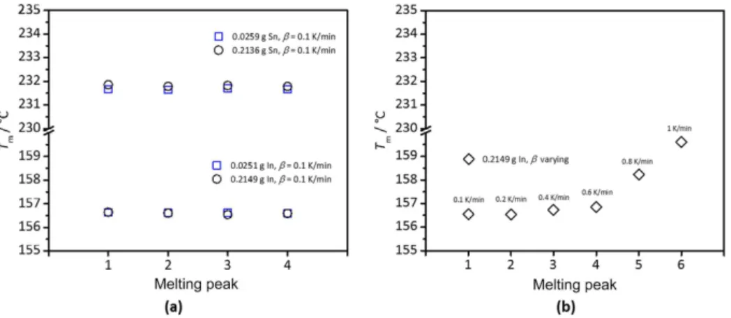
Figure 8.Comparison between the melting temperatureTmin literature of indium and tin and data determined during experiments with a
constant heating rate of 0.1 K min−1(a)and the variation of the heating rate for one indium sample(b).
β, which is indicated by the peak height and the smaller peak widths.
The temperature of the sample during the experiment was monitored by the Pt500 resistor in the cuvette which was calibrated in a prior measurement to the melting peak of indium at a heating rate of β=0.1 K min−1. The melting temperature was defined as the temperature of the onset of the melting peak. For indium, Fig. 8a shows the good agreement of the measured melting temperatures with lit-erature (Cammenga et al., 1993). The total standard devia-tion of the determined temperatures for both indium masses of was 32 mK with an average of 156.6045◦C, which is a deviation of approximately 6.0 mK from the literature value of Tm,In,lit=156.5985◦C. For tin those data are a bit higher with a standard deviation of the melting temperature 80 mK at an average of 231.7409◦C, which is a deviation to
Tm,Sn,lit=231.928◦C of 187.1 mK. This is still a good value for a single point calibration, especially for such a device, as the sample is about 0.8 cm away from the cuvette and about 0.9 cm from the thermocouples of the sensor. It can be con-cluded that the measurement of the melting temperature is very accurate for the device. When the heating rate is in-creased (Fig. 8b), the temperature lag between sample and measuring point increases too. This makes the temperature calibration dependent on the heating rate. In this case the cal-ibration for 0.1 K min−1is still valid at 0.2 K min−1, but not at 0.4 K min−1. On this effect Sarge et al. (1997) have already reported for similar devices.
As shown in the inset in Fig. 7, the measured absolute value for the enthalpy of fusion for each peak, 1fust H, is obtained by integrating the peak area over time. Divid-ing the resultDivid-ing values by the mass of the sample yields the specific heat of fusion, 1fush. Figure 9 shows values for all measurements, proofing that this device is able to measure specific enthalpies of melting and fusion of in-dium and tin with good precision. For the higher masses of about 210 mg of tin and indium, the fluctuation range
Figure 9.Data of the melting enthalpies1fushof tin, and indium
obtained from experiments where the samples melted (m.) or solid-ified (s.).
1fushIn,mean=30.09 J g−1is 8.5 % higher than the literature value of 1fushIn,lit=28.62 J g1 reported by Della Gatta et al. (2006).
As it is observed that both measured values are higher than the literature value, it is assumed that this is a flaw in the calibration process for the device. This is underlined by the high accuracy of the measurements. One possible explana-tion is the fact that the heat during calibraexplana-tion was impressed through the cylindrical surface of a cuvette and the measured samples have a point-like geometry. Thus, a smaller propor-tion of heat is lost during measurement of the samples than during calibration with the cuvettes. This increases the cal-culated heats.
4 Conclusion and outlook
In this work, we have shown that a validated model of a Tian– Calvet calorimeter can help to improve the sensitivity of the sensor. Best results have been achieved by printing thermo-couples on both sides of the sensor discs, thus eliminating the need for cutouts in the sensor. Additionally, tolerances in diameter of the sensor could be identified as a crucial pa-rameter. After improving the manufacturing processes, the sensitivity could be increased by the factor of 3 compared to the initial design. First measurements with the new sensor were conducted to calibrate the device between room temper-ature and 300◦C, using calibration cuvettes to impress pow-ers of 1 and 100 mW. As expected, the sensitivity increases with sample temperature but is independent of the applied power. As a final proof, melting enthalpies of indium and tin were measured in a scanning modus with a heating rate of β=0.1 K min−1. The melting temperature for indium could be determined with an accuracy better than 1/100 K and of tin with an accuracy better than 2/10 K. Both are good values for such a device. The value for tin may even be improved by a calibration in this temperature range. Melting enthalpies have been determined with a precision of 1 % for most sam-ples. The accuracy of the melting enthalpy for indium was about 8.5 %, while the measurements for tin reached 2 %. It can be stated that this can be improved by more elaborated calibration processes. Future work will focus on processes to further calibrate the device and expand its temperature range.
Acknowledgements. The presented results have been achieved in the scope of the project MST-1304-0003//BAY182/002 “High-Resolution Calorimetric Sensor”, which is funded by the Bavarian Ministry of Economic Affairs and Media, Energy and Technology, VDI/VDE-IT Microsystems Technology Program.
Edited by: T. Fröhlich
Reviewed by: two anonymous referees
References
Auroux, A.: Calorimetry and Thermal Methods in Catalysis, Springer Series in Materials Science, 154, Springer, Berlin, Hei-delberg, ISBN-13: 978-3-642-11953-8, 2013.
Calvet, E. and Prat, H.: Recent progress in microcalorimetry, Perg-amon Press, Oxford, ISBN-13: 978-0-08-010032-6, 1963. Cammenga, H. K., Eysel, W., Gmelin, E., Hemminger, W.,
Höhne, G. W., and Sarge, S. M.: The temperature calibration of scanning calorimeters, Thermochim. Acta, 219, 333–342, doi:10.1016/0040-6031(93)80510-H, 1993.
Della Gatta, G., Richardson, M. J., Sarge, S. M., and Stølen, S.: Standards, calibration, and guidelines in microcalorimetry. Part 2. Calibration standards for differential scanning calorimetry (IUPAC Technical Report), Pure Appl. Chem., 78, 1455–1476, doi:10.1351/pac200678071455, 2006.
Gongora-Rubio, M., Espinoza-Vallejos, P., Sola-Laguna, L., and Santiago-Avilés, J.: Overview of low temperature co-fired ce-ramics tape technology for meso-system technology (MsST), Sensor. Actuat. A-Phys., 89, 222–241, doi:10.1016/S0924-4247(00)00554-9, 2001.
Gotoh, M., Hill, K. D., and Murdock, E. G.: A gold/platinum thermocouple reference table, Rev. Sci. Instrum., 62, 2778, doi:10.1063/1.1142213, 1991.
Höhne, G., Hemminger, W., and Flammersheim, H.-J.: Differential scanning calorimetry: An introduction for practitioners, 2nd ed., Springer, Berlin, New York, xii, 298 pp., 2003.
Imanaka, Y.: Multilayered low temperature cofired ceramics (LTCC) technology, Springer, New York, ISBN-13: 978-0-387-23314-7, 2005.
Kita, J. and Moos, R.: Development of LTCC-materials and their applications – an overview, Informacije MIDEM, 38, 219–224, 2008.
Kita, J., Rettig, F., Moos, R., Drue, K.-H., and Thust, H.: Hot Plate Gas Sensors-Are Ceramics Better?, Int. J. Appl. Ceram. Tec., 2, 383–389, doi:10.1111/j.1744-7402.2005.02037.x, 2005. Peralta-Martinez, M. V. and Wakeham, W. A.: Thermal
Conductiv-ity of Liquid Tin and Indium, Int. J. Thermophys., 22, 395–403, doi:10.1023/A:1010714612865, 2001.
Sarge, S. M., Gmelin, E., Höhne, G. W., Cammenga, H. K., Hemminger, W., and Eysel, W.: The caloric calibration of scanning calorimeters, Thermochim. Acta, 247, 129–168, doi:10.1016/0040-6031(94)80118-5, 1994.
Sarge, S. M., Hemminger, W., Gmelin, E., Höhne, G. W. H., Cam-menga, H. K., and Eysel, W.: Metrologically based procedures for the temperature, heat and heat flow rate calibration of DSC, J. Therm. Anal., 49, 1125–1134, doi:10.1007/BF01996802, 1997. Sarge, S. M., Höhne, G. W., Cammenga, H. K., Eysel, W., and
Gmelin, E.: Temperature, heat and heat flow rate calibration of scanning calorimeters in the cooling mode, Thermochim. Acta, 361, 1–20, doi:10.1016/S0040-6031(00)00543-8, 2000. Schubert, F., Gollner, M., Kita, J., Linseis, F., and Moos, R.:
First steps to develop a sensor for a Tian-Calvet calorime-ter with increased sensitivity, J. Sens. Sens. Syst., 5, 205–212, doi:10.5194/jsss-5-205-2016, 2016.