How Entorhinal Grid Cells May Learn Multiple Spatial
Scales from a Dorsoventral Gradient of Cell Response
Rates in a Self-organizing Map
Stephen Grossberg*, Praveen K. Pilly
Center for Adaptive Systems, Graduate Program in Cognitive and Neural Systems, and Center for Computational Neuroscience and Neural Technology, Boston University, Boston, Massachusetts, United States of America
Abstract
Place cells in the hippocampus of higher mammals are critical for spatial navigation. Recent modeling clarifies how this may be achieved by how grid cells in the medial entorhinal cortex (MEC) input to place cells. Grid cells exhibit hexagonal grid firing patterns across space in multiple spatial scales along the MEC dorsoventral axis. Signals from grid cells of multiple scales combine adaptively to activate place cells that represent much larger spaces than grid cells. But how do grid cells learn to fire at multiple positions that form a hexagonal grid, and with spatial scales that increase along the dorsoventral axis? In vitro recordings of medial entorhinal layer II stellate cells have revealed subthreshold membrane potential
oscillations (MPOs) whose temporal periods, and time constants of excitatory postsynaptic potentials (EPSPs), both increase along this axis. Slower (faster) subthreshold MPOs and slower (faster) EPSPs correlate with larger (smaller) grid spacings and field widths. A self-organizing map neural model explains how the anatomical gradient of grid spatial scales can be learned by cells that respond more slowly along the gradient to their inputs from stripe cells of multiple scales, which perform linear velocity path integration. The model cells also exhibit MPO frequencies that covary with their response rates. The gradient in intrinsic rhythmicity is thus not compelling evidence for oscillatory interference as a mechanism of grid cell firing. A response rate gradient combined with input stripe cells that have normalized receptive fields can reproduce all known spatial and temporal properties of grid cells along the MEC dorsoventral axis. This spatial gradient mechanism is homologous to a gradient mechanism for temporal learning in the lateral entorhinal cortex and its hippocampal projections. Spatial and temporal representations may hereby arise from homologous mechanisms, thereby embodying a mechanistic ‘‘neural relativity’’ that may clarify how episodic memories are learned.
Citation:Grossberg S, Pilly PK (2012) How Entorhinal Grid Cells May Learn Multiple Spatial Scales from a Dorsoventral Gradient of Cell Response Rates in a Self-organizing Map. PLoS Comput Biol 8(10): e1002648. doi:10.1371/journal.pcbi.1002648
Editor:Olaf Sporns, Indiana University, United States of America
ReceivedJanuary 24, 2012;AcceptedJune 20, 2012;PublishedOctober 4, 2012
Copyright:ß2012 Grossberg, Pilly. This is an open-access article distributed under the terms of the Creative Commons Attribution License, which permits unrestricted use, distribution, and reproduction in any medium, provided the original author and source are credited.
Funding:This work was supported in part by the SyNAPSE program of DARPA (HR0011-09-C-0001). The funders had no role in study design, data collection and analysis, decision to publish, or preparation of the manuscript.
Competing Interests:The authors have declared that no competing interests exist.
* E-mail: [email protected]
Introduction
A gradient of spatial scales in medial entorhinal cortex Navigating the world requires the brain to learn and maintain memory of spatial positions within various environments. Place cells in the hippocampal areas CA1 and CA3 demonstrate a neural code for position in large spaces that higher mammals inhabit [1] and thereby play a critical role in spatial navigation. CA3 receives major projections from layer II of the medial entorhinal cortex (MEC) [2], where grid cells are predominant [3,4]. Unlike place cells, individual grid cells fire at multiple positions. When an animal navigates in an open field, these positions form a regular hexagonal grid uniformly covering the entire navigable environment. These cells are found throughout the length of MEC with the spatial period of their firing fields increasing from the dorsomedial to the ventrolateral end [4–6].
In particular, Brun and colleagues [6] recorded from a total of 143 grid cells within layers (II, III, V/VI) of MEC located between 1% to 75% the distance along the dorsoventral axis, while rats ran back and forth on a 18 m long linear track. The recorded cells were divided into three groups based on their anatomical location
with respect to the postrhinal border of MEC; namely, dorsal, intermediate and ventral. The one-dimensional periodic spatial responses of these cells in the two running directions were processed separately to estimate characteristic properties of grid cells, such as grid spacing, grid field width, peak firing rate, and mean firing rate. The main finding was that both grid spacing and field width increased from dorsal group to ventral group, for either running direction. Interestingly, distributions of these variables increased not only in mean but also in variability with distance along the dorsoventral axis. However, the peak firing rate decreased from dorsal group to ventral group, and there was a negative trend for mean firing rate.
to place cells arises due to the fact that the SOM is sensitive to the most frequent coactivations of grid cells across multiple scales, which on a linear track occur with a spatial period equal to the least common multiple of the inducing grid spacings. But how do grid cells learn to fire at multiple positions that form a hexagonal grid in two-dimensional open environments? And how does the spatial scale of grid cells increase along the dorsoventral axis of MEC, enabling their target place cells to represent ever-larger spaces? Recent data and modeling provide some clues, forming the basis for the current work.
Correlating stellate cell oscillation frequency with grid cell spatial scale
Excitatory projections to the hippocampal formation from layer II of MEC are primarily from stellate cells [12]. That makes them the most likely candidates for grid cells. In vitrowhole-cell patch clamp recordings [13,14] have shown that these stellate cells exhibit subthreshold membrane potential oscillations (MPOs) in response to steady current injection. The temporal period of these oscillations increases from the dorsomedial to the ventrolateral end of MEC, thereby correlating with the observed gradient in spatial period and size of the firing fields of grid cells. In addition, voltage-clamp recordings in these cells demonstrated that the time constants of the hyperpolarization-activated cation current ð ÞIh decreases along the dorsoventral axis of MEC
[15,16]. Knockout of the HCN1 subunit in the hyperpolariza-tion-activated cyclic nucleotide-gated (HCN) channels, which controlIhkinetics [17], flattens the dorsoventral gradient of MPO
frequency [18]. In addition, the rise and fall times of excitatory postsynaptic potentials (EPSPs) in these cells progressively become longer along the dorsoventral axis [19]. The variation in EPSP kinetics was attributed to differences in the membrane conductance mediated by HCN and leak potassium channels. Combined, all these results suggest a correlation between the rate of intrinsic dynamics in MEC layer II stellate cells and the spatial scale of grid cells.
Model accomplishments
This article develops a SOM neural model, called Spectral Spacing for reasons summarized below, to explain the above data.
This model shows how a gradient of cell response rates along the dorsoventral axis of MEC can control the development of grid cells whose hexagonal grid firing fields exhibit a gradient of spatial scales and whose MPOs exhibit a gradient of frequencies. These results combine several conceptual and technical advances.
First, these results are part of an emerging general entorhinal-hippocampal model architecture (see also [20]), which shows that, despite their different receptive field structures, both grid cells and place cells may be learned using the same SOM laws. Thus, both grid cell periodic hexagonal firing fields and place cell unimodal firing fields, despite their different appearances, may arise from the same neural mechanisms due to the different inputs that they receive at their respective stages in the entorhinal-hippocampal hierarchy.
Second, these SOM laws have been proposed to control development and learning in many other parts of the brain, notably the visual cortex. Thus, both grid and place cells may develop using general SOM principles of brain map organization. Third, the linear velocity and angular velocity path integration inputs that drive model learning are derived from realistic trajectories of rats in spatial learning and memory experiments.
Fourth, these linear velocity and angular velocity estimates can both be transformed into position codes by ring attractors.
Fifth, the rate gradient mechanism for spatial learning in the MEC pathway and its hippocampal projections is homologous to a rate gradient mechanism that has been used to model temporal learning in the lateral entorhinal cortex (LEC) pathway and its hippocampal projections. Spatial and temporal representations in the medial and lateral processing streams may hereby arise from homologous mechanisms, thereby embodying a mechanistic ‘‘neural relativity’’ in the entorhinal-hippocampal system. This homology may clarify why spatial and temporal representations both occur in hippocampus, and provides new clues about how episodic memories may be learned.
In summary, this model system exhibits parsimony and unity, both in its use of similar ring attractor mechanisms to code the linear and angular velocity path integration inputs that drive learning, and in its use of a rate gradient mechanism that can support the learning of both spatial and temporal codes.
Even more striking is the fact that both grid cell and place cell receptive fields emerge by detecting, learning, and remembering the most frequent and energetic coactivations of their inputs. This co-occurrence property is different from the property of oscillatory interference that some other models have proposed (e.g., [21]). Oscillatory interference models have, to the present, been used to explain properties of grid cells, without showing how they can be learned, or how such a learning process can generate the different grid spatial scales along the dorsoventral extent of MEC. Moreover, several articles (e.g., [13,22]) have interpreted the gradient of subthreshold MPO frequencies in MEC layer II stellate cells as strong evidence for an oscillatory interference-based firing of grid cells. In sharp contrast, the grid cells in the Spectral Spacing model exhibit the gradient of MPO frequencies as an epiphenomenon of SOM learning mechanisms, thereby showing that this gradient can occur in the absence of an oscillatory interference mechanism.
In order to better understand what aspects of the Spectral Spacing model are needed to explain how spatial and temporal properties of grid cell firing change along the dorsoventral extent of MEC, several model and input variations were simulated (see
Simulation Settings). These simulations demonstrate that, at least among these variations, only a response rate gradient, combined with input cells that have normalized receptive fields, can explain all the data mentioned above.
Author Summary
Stripe cells and ring attractors
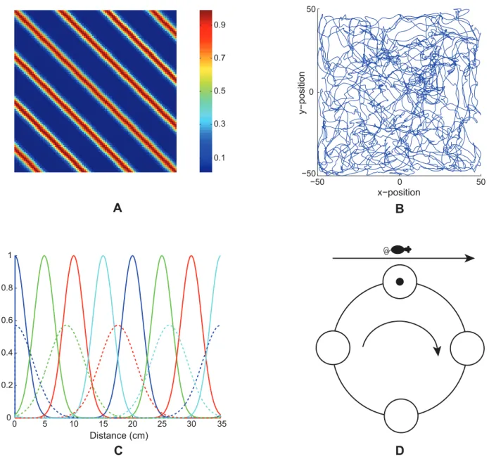
The input cells to the grid cells are calledstripe cells[23]. They are called stripe cells because each cell fires with a preferred movement direction and spatial period, thereby giving rise to stripes of activation (Figure 1A). Suggestive data about these cells in deeper layers of MEC were reported in [4]. In addition, Krupic, Burgess, and O’Keefe [24] have reported data showing stripe-like spatial firing profiles for a group of cells in the dorsal parasubiculum, which projects to layer II of MEC [25,26].
In the GRIDSmap model [23] and the Spectral Spacing model simulations, the stripe cells process linear velocity inputs that are modulated by head direction as the model animal navigates a realistic trajectory that was reported in the data of [4]; see Figure 1B. These signals are assumed to be computedin vivofrom vestibular estimates of linear and angular acceleration, which are
generated in the otolithic organs and semicircular canals, respectively, of the inner ears [27].
In addition to its preferred direction and spatial scale, each stripe cell is assumed to have a preferred spatial phase (Figure 1C). A set of stripe cells for a given direction and spacing, which differ only in spatial phase, can be represented by cells constituting a one-dimensional ring attractor (Figure 1D). In such a ring attractor, linear velocity projected onto the preferred direction moves an activity bump around the ring of stripe cells (see Figure 1D and Equations 1.1–1.4). One revolution of the activity bump corresponds to traversal of a length equal to the associated stripe spacing along the direction (Figure 1A). The spatial firing of a stripe cell as the animal moves at a constant speed on a straight path is assumed to have a Gaussian profile, for simplicity, with different stripe cells in the ring having different spatial offsets for
Figure 1. Linear path integration inputs.(A) Spatial response of a model stripe cell with a spacing of 20 cm in a 100 cm6100 cm environment. (B) Realistic rat trajectory in the same sized environment used in our simulations (data: [4]). (C) Small-scale (solid; spacing of 20 cm) and large-scale (dashed; spacing of 35 cm) stripe fields of four spatial phases (colors) along their preferred direction. Note the normalized stripe fields; that is, the area under each stripe field is a constant between the two scales. (D) Depiction of how the bump of activity in each directional ring attractor can be moved by linear movements of an animal with a component along the preferred direction.
their peak firing. The movement of the activity bump depends on the component of linear velocity along the associated direction. As a result, the spatial firing pattern of a given stripe cell in a two-dimensional environment resembles Gaussian-modulated oriented stripes with a fixed spacing that uniformly spread across the entire environment (Figure 1A). Because of the periodic boundary condition, each stripe cell operates over a limited spatial scale equivalent to the spacing between its adjacent stripe fields.
As noted above, each stripe cell ring attractor includes cells that are sensitive to a given spatial scale, both spatial period and spatial phase, and movement direction. The set of all stripe cells, across all spatial periods, spatial phases, and directions, taken together, implicitly represent the spatial position of the animal. In particular, stripe cells of different spacings can represent the animal’s position at multiple spatial resolutions.
Head direction cells and ring attractors
The firing of a stripe cell with a prescribed directional preference is modulated by a head direction signal via a cosine law that projects the current direction of the navigating animal at each time onto the stripe cell’s preferred direction (see Equation 1.1). Head direction estimates have been modeled by ring attractors that are sensitive to angular velocity signals [28–35]. Both linear velocity and angular velocity signals in the Spectral Spacing model are thus assumed to be transformed into movements of activity bumps in ring attractors in order to perform linear and angular path integration, respectively (cf. [23,36]). Adult-like head direction cells are already present in the parahippocampus by P16 when rat pups begin to explore their environments for the first time [37,38]. If both stripe cells and head direction cells are indeed computed by ring attractors, then this provides a plausible explanation of how stripe cells could be ready at this developmental stage to support the learning of grid cells.
SOM dynamics and learning
Stripe cells with multiple directional preferences and spatial phases for a given spatial period initially project with random adaptive weights to cells in the category learning layer of a SOM. SOM cells obey membrane, or shunting, equations and interact in a recurrent on-center off-surround network. Self-excitatory feed-back enables the resolution of competition among the map cells in order to choose one or a few winners. The self-excitatory feedback does this by contrast-enhancing the activity of winning category cells [39], but it can also cause perseveration of activity in the winning cells, even after their bottom-up inputs shut off. A perseverating cell could inhibit other map cells, via the recurrent off-surround, that would be needed to represent different combinations of inputs that arise as an animal continues to navigate. Activity-dependent habituative gating of the positive feedback signals causes a collapse of such persistent self-activation, and thereby allows different map cells to become active and learn at different times as the bottom-up stripe cell input pattern changes with the animal’s navigational movements in space. In other words, habituative gating helps to ‘‘whiten’’ the learned spatial fields of the map cells. Habituative gating has been used in SOM models of other parts of the brain since being introduced in [40]. It has helped, for example, to simulate complex properties of map development in visual cortical area V1 (e.g., [41–43]).
Signals from winning map cells trigger learning in the abutting synapses of pathways from the stripe cells. The adaptive weights in these synapses track a normalized time-average of the signals in the pathways from the stripe cells while their target map cells are
active. After learning, the bottom-up signals can efficiently activate map cells that exhibit hexagonal grid fields.
In addition to these basic SOM ingredients, the current model investigates how a gradient of response rates in the map cells can lead to learning of a gradient of model grid cell spatial scales whose properties match neurophysiological data from multiple experi-ments about grid cells along the dorsoventral axis of the MEC. See the subsection below on theScale selection problem.
The learning law is called acompetitive instar learning lawbecause it selectively strengthens the adaptive weights from coactive stripe cells to active map cells while it competitively self-normalizes the total adaptive weight abutting each map cell [40,41,44,45]. This learning law enables each grid cell to arise as a learned spatial category in a SOM. The competitive aspect in the learning law may be interpreted in terms of how developing axons abutting a target neuron compete for limited target-derived neurotrophic factor support in order to survive [46–48], and its conservation of total synaptic weight is consistent with neurobiological data (e.g., [49]).
Such a competitive instar learning law is different from a purely Hebbian learning law, which allows adaptive weights to increase but does not allow them to decrease. The instar learning law permits both weight increases (long-term potentiation) and weight decreases (long-term depression). It hereby enables the weights to adapt to the spatial pattern of signals from the stripe cells. This pattern sensitivity enables grid cell learning to become sensitive to temporal co-occurrences of stripe cell firing.
Simultaneously active stripe cells are more likely to strongly activate map cells whose bottom-up weight patterns closely match their activity pattern. Adaptation of the weights to a map cell occurs only when its activity is above a threshold (see C in Equation 1.6). This postsynaptic activity-based gating ensures faster adaptation of incoming weights for more active map cells. During each learning episode, the weights tend towards the average normalized pattern of the inputs. Thus, the likelihood of the map cells becoming tuned to particular sets of inputs, which consistently succeed in driving them, gradually increases. Note that the bottom-up connections from stripe cells to grid cells remain adaptive for the lifetime of the animal, and not just during the development period.
SOM hierarchy: From stripe cells to place cells via grid cells
Until recently, SOM models of place cell learning used idealized or hand-crafted grid cells (e.g., [10,11]). Pilly and Grossberg [20] proposed the GridPlaceMap model to show how grid and place receptive fields, despite their different characteristics, can emerge simultaneously at different levels in a SOM hierarchy, obeying the same laws for neuronal dynamics and synaptic plasticity, by responding to the most frequent and energetic coactivations of their corresponding input neurons. This medial entorhinal-hippocampal hierarchy of stripe, grid, and place cells enables the brain to represent increasingly large spaces, and provides increasingly large spatial information per cell in predicting the spatial position of an animal.
Scale selection problem
Both the GRIDSmap and the GridPlaceMap models learn hexagonal grid firing fields whose spatial scale is derived from that of the input stripe cells. In particular, stripe cells with the same period were used to learn grid fields of a given spatial scale. Stripe cells of different spatial scales were assumed to activate different locations along the dorsoventral axis in layer II of MEC, thereby giving rise to grid cells with different spatial scales. But how is the selection of just one spatial scale of stripe cells realized for each grid cell scale? What would happen if stripe cells of multiple scales
initially projected to the map layer before grid cell learning began, as in Figure 2? In other words, how do grid cells learn to select among, not only multiple directional preferences and spatial phases, but also among the multiple spatial scales, of their stripe cell inputs? What properties of the dynamics of a map cell can select the spatial scale to which it will learn to respond as a grid cell?
Cell response rates select grid cell spatial scale and controls MPO frequency
This article shows that the rates at which the category cells and their corresponding habituative transmitters respond, called the response rate (parametermmin Equation 1.5) and habituation rate (parametergmin Equation 1.7), respectively, can help to select the spatial scale of the stripe cells to which the category cells will learn to respond, and thus the spatial scale of the learned hexagonal grid firing fields, as well as the MPO frequencies with which these grid cells respond in vitro to a steady current input. Whereas a dorsoventral gradient in either response rate or habituation rate can explain the corresponding gradient in learned spatial scale and MPO frequency of grid cells, only a gradient in response rate was found to be consistent with data regarding the associated dorsoventral gradient in peak and mean firing rates of grid cells [6]; see the Results section for details. Different cell response rates also indirectly alter the rates at which the habituative transmitters inactivate and recover (see Figure 3D).
Figure 2. Model depiction.The Spectral Spacing model responds to the navigational movements of an animal along a realistic trajectory and with stripe cells of multiple spatial scales initially projecting to the population of category learning cells at some location along the dorsoventral axis of MEC. Model simulations were conducted with 25 category cells in each of 10 MEC local populations that differed in the rate of intrinsic cellular dynamics, and with input stripe cells of nine directional preferences, four spatial phases, and up to three spatial scales.
Figure 3. Case 1 results.Results of Case 1 in which a single category cell responded to a stripe cell-like input S(t)~e{(t{0:695)2 0:0627
shown in (A). (B)
Cell responses defined by Vm j {C
h iz
2
for different response rates (mm: 1 (cyan), 0.5 (red), 0.2 (green), and 0.1 (blue)) in the absence of
self-excitatory feedback. Here, cell potential Vm j
follows:dV m j
dt ~10mm {AV m j z B{V
m j
S ð Þ
h i
. (C) Cell responses defined by Vm j {C
h iz
2
in the
p r es ence of s el f - ex c ita t or y f e edb ack t ha t is n ot ha bi tua t iv el y gate d. In t his c a s e, c ell pote nti al Vm j
f o l l o w s :
dVm j
dt ~10mm {AV m
j z B{Vjm
Sza Vm j h iz
2!
" #
. (D) Dynamics of the habituative transmitter zm j
in the presence of self-excitatory
feedback that is habituatively gated. (E) Cell responses defined by the habituatively gated product Vm j h iz
2
zm
Spectral Timing and Spectral Spacing
Remarkably, this response rate gradient forspatiallearning is computationally homologous to a rate gradient that was proposed over 20 years ago to explain hippocampal data about
temporallearning [50–52]. The model for temporal learning was called a Spectral Timing model because its different cell populations respond with a ‘‘spectrum’’ of different rates. The current model may therefore be called a Spectral Spacing model. Whereas the rate gradient for spatial learning is proposed to occur in MEC and its hippocampal projections, the rate gradient for temporal learning is proposed to occur in LEC and its hippocampal projections. This homology may provide new clues about how episodic memories are learned. See the
Discussionsection for further comments about this predicted form of ‘‘neural relativity’’ in the entorhinal-hippocampal system.
Methods
The Spectral Spacing model that is developed in this article significantly refines and modifies the GRIDSmap model of [23] to explain how a cell response rate gradient [19] can generate learning of a gradient in grid cell spatial scale [5,6] from among multiple spatial scales of input stripe cells. In addition, the learned grid cells exhibit activity patterns whose properties simulate data about the gradient of MPO frequency [13,14] and of peak and mean firing rates [6] along the dorsoventral axis in layer II of MEC. The Spectral Spacing model also computa-tionally investigates different variations of stripe cell properties (peak firing rate, stripe field width) across spatial scales to predict what may be observed in future experiments. Besides these major conceptual advances, the Spectral Spacing model also incorporates several technical advances over the GRID-Smap model that enable it to learn a greater number of stable grid cells in a larger population of self-organizing cells; see the
Differences with GRIDSmap model subsection in the
Discussionsection.
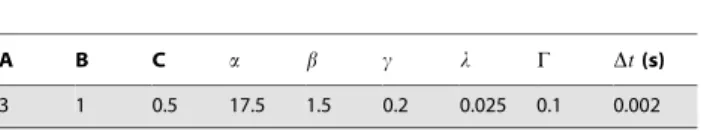
We first provide below a complete mathematical description of the Spectral Spacing model and its variations. The values of parameters that do not differ across simulation cases are listed in Table 1. The values for the other parameters are specified in the
Simulation Settingssubsection below. Table 2 lists experimen-tal evidence in support of the various model components. Numerical integration was performed using Euler’s forward method with a fixed time stepDt.
Spectral Spacing model equations
Stripe cells. As noted above, stripe cells integrate linear velocity in multiple directions, spatial phases, and spatial scales in ring attractor circuits. They are algorithmically computed, for simplicity, as follows [23]: If at time t an animal heads along allocentric directionQð Þt with velocityv tð Þ, then the velocityvdð Þt
along directiond is:
vdð Þt~cosðd{Qð Þt Þv tð Þ: ð1:1Þ
The displacementDdð Þt traversed along directiondwith respect
to the initial position is calculated by path integration of the corresponding velocity:
Ddð Þt~ ðt
0
vdð Þtdt: ð1:2Þ
This directional displacement variable is converted into activa-tions of stripe cells that prefer different spatial phasespalong a ring attractor that is selectively tuned to directiondand spatial scales. Let xdpsð Þt be the activity of a stripe cell whose spatial
fields are oriented perpendicular to direction d with spatial phase p and spatial period s. This stripe cell has maximal activity at periodic positions nszp along direction d, for all integer values ofn; see Figure 1A. Activityxdpsð Þt will thus be
maximal whenever (Dd modulo s) =p, where the modulo
operator computes the remainder when Dd is divided by s,
and thus resets the displacement modulo the period s. This periodically reset displacement, computed with respect to spatial phasepis:
Ddpsð Þt ~ðDdð Þt {pÞmodulos: ð1:3Þ
Thus, if the stripe cellxdpsð Þt has a Gaussian-like spatial firing
profile, then its activity can be modeled as:
xdpsð Þt~rs:exp {
min Ddpsð Þt,s{Ddpsð Þt
2
2ss2
!
, ð1:4Þ
wherersis the maximal activity andssis the standard deviation
of each of its individual stripe fields along the directiond. The simulations were carried out with two, or three, spatial scaless of stripe cells converging on individual category cells. Learning determines which stripe cell spatial scale gains control of each category cell through time, and how that results in its learned grid scale. Simulations demonstrate how the response rate of a category cell determines its learned grid scale. The directional displacement variablesDdð Þt were all initialized to 0 at the start
of each learning trial.
Category cells. The membrane potential Vm
j of the MEC
layer II category celljin populationmalong the dorsoventral axis obeys shunting dynamics within a recurrent on-center off-surround network [40,44]. The membrane potential Vm
j of the
defined by Vm
j {C
h iz
2
for the case in (D). For (D–F), cell potential Vm j
and habituative transmitter zm j
follow
dVm j
dt ~10mm {AV m j z B{V
m j
Sza Vjm
h iz
2
zmj !
" #
anddz m j
dt ~10gm 1{z m j
{czmj a Vjm
h iz
2!2
0
@
1
A, respectively.
doi:10.1371/journal.pcbi.1002648.g003
Table 1.Values of model parameters that do not differ across
various simulation cases.
A B C a b c l C Dt(s)
3 1 0.5 17.5 1.5 0.2 0.025 0.1 0.002
jthcell in populationmtherefore obeys the equation:
dVm j
dt ~10mm {AV m
j z B{V m j
X
dps
wmdpsjxdpsz "
a hVjmi z
2
zmj !
{CzVjm X k=j
bVkm{C z2 #
z
snoise dW
dt :
ð1:5Þ
The model was run in several variations to demonstrate the effects of gradients in cell response rates or habituation rates. This analysis points to the fact that a gradient of response ratesmm, with all other parameters held fixed, leads to learned grid cells that best match neurophysiological data. Thus, in one set of simulations, 10 non-interacting populations of category cells, each with 25 cells, were assumed to occur at different anatomical locations on the dorsoventral axis. The only parameter that was varied across these populations was the response ratemm, with values of 1, 0.9, 0.8, 0.7, 0.6, 0.5, 0.4, 0.3, 0.2, and 0.1. This is similar to the anatomical gradient of response rates proposed in the Spectral Timing model to account for the learning of adaptively timed behaviors [50].
In Equation 1.5,Ais the decay parameter corresponding to the leak conductance; Band {C are the reversal potentials of the excitatory and inhibitory channels, respectively; wm
dpsj is the
synaptic weight of the projection from the stripe cell with activity xdps in Equation 1.4 to the category cell j in population m;
a Vm j h iz
2
is the on-center self-excitatory feedback signal of the
cell, which helps to resolve the competition among category cells within cell population m, where ½ Vz
~maxðV,0Þ defines a threshold-linear function, andais the gain coefficient;zm
j is the
habituative transmitter gate of category cellj;bis the connection
strength of the inhibitory signal Vm k{C
z
2
from category cell
kin the off-surround to category celljwithin populationm; and
term snoisedW
dt injects additive noise into the cellular dynamics, where W is a Brownian motion process with independent increments sampled from a Gaussian distribution with zero mean and standard deviation equal tosnoise. At each time step (Dt) of numerical integration, a zero mean Gaussian random variable of variances2
noiseDtis added to the cell potential. The output activity
of category celljis given by Vm j {C
h iz
2
, which is the same as
its recurrent inhibitory signal to other cells in the population. The membrane potential of each category cell was initialized to 0 at the start of each learning trial.
Adaptive weights. The adaptive weightswm
dpsjof projections
from stripe cells to category cells are governed by a variant of the competitive instar learning law [40,41]:
dwm dpsj dt ~l V
m j {C
h iz
2
1{wm dpsj
xdps{wmdpsj X
p,q,r ð Þ=ðd,p,sÞ
xpqr 2
4
3
5,
ð1:6Þ
where l is the learning rate; the category cell output signal
Vm j {C
h iz
2
gates learning on and off; and the learning rule
defines a self-normalizing competition among afferent synaptic weights to the target cell, leading to a maximum learned total weight to the cell of 1. Each weight wm
dpsj was initialized to a
random value drawn from a uniform distribution between 0 and 0.1 at the start of the first learning trial.
Equation (1.6) can be rewritten with term 1{wm dpsj
xdps{ h
wm dpsj
P
p,q,r ð Þ=ðd,p,sÞ
xpqr
replaced by xdps{wmdpsj Pp,q,r ð Þ
xpqr !
, which
Table 2.List of experimental evidence for various model components.
Model component Equation reference Experimental evidence
Stripe cells in parasubiculum (preliminary SfN abstract)
xdpsin Equation 1.5 [24]
Anatomical projections from parasubiculum to layer II of MEC
P
dps
wm
dpsjxdpsin Equation 1.5 [25,26]
Dorsoventral gradient in the rate of temporal summation of MEC layer II stellate cells
mmin Equation 1.5 [19]
Self-excitatory feedback in MEC layer II stellate cells based on a Ca2+-sensitive nonspecific cation current (ICAN)
z B{Vm j
a Vm j
h iz
2!
in Equation 1.5
[53,54]
Inhibitory interneurons in layer II of MEC
{ CzVm j
P
k=j
b Vm
k{C
z
2
in Equation 1.5 [55]
Adaptation in MEC layer II stellate cells related to Ca2+-dependent K+(AHP) currents
zm
j in Equation 1.5; and Equation 1.7 [56]
Competition among developing axons abutting a map cell
{wm dpsj
P
p,q,r ð Þ=ðd,p,sÞ
xpqrin Equation 1.6 [47,48]
Conservation of total synaptic weight P
dps
wm
dpsj~1when Equation 1.6 converges [49]
Postsynaptic activity-dependent plasticity
Vm
j{C
h iz
2
in Equation 1.6 [57]
shows that the weight wm
dpsj is attracted to a time-average of the
ratio of input activities during the times when the gating, or
learning, signal Vm j {C
h iz
2
is positive. This fact embodies the
intuition that the learning law conserves the total number of synaptic learning sites at each map cell by a homeostatic combination of excitatory and inhibitory influences.
Habituative gating. The habituative transmitterzm j of
cate-gory celljin populationmis defined by:
dzm j
dt ~10gm 1{z m j
{czmj a Vjm h iz
2!2
2
4
3
5: ð1:7Þ
In Equation 1.7,gmdetermines the response rate of the transmitter dynamics (called the habituation rate) andcmodulates the depletion rate of the transmitter. The habituative transmitter of each category cell was initialized to its maximum value of 1 at the start of each learning trial.
Intuitively, Equation 1.7 says that the transmitterzm
j is depleted,
or inactivated, via mass action by the signal that it gates (see
Equation 1.5). In particular, term 1{zmj
controls the gate
recovery rate to the target level of 1, and term
{czm
j a Vjm h iz
2!2
controls the gate inactivation rate, which
is proportional to the current gate strengthzjtimes the square of
the signal a Vm j h iz
2!
that zm
j gates in Equation 1.5. The
squaring operation causes the gated signal to first increase and then decrease through time in response to excitatory input (cf., [58]), thereby limiting the duration of intense cell activity, and thus cell perseveration. This duration is inversely proportional to both the response ratemm (see Figure 3F) and the habituation rategm.
Post-processing
The 100 cm6100 cm environment was divided into 2.5 cm62.5 cm bins. During each learning trial, the amount of time spent by the navigated trajectory in the various spatial bins was tracked. The output activity of each category cell in every spatial bin was accumulated as the trajectory visited that bin. The occupancy and activity maps were smoothed using a 565 Gaussian kernel with standard deviation equal to one. At the end of each learning trial, smoothed and unsmoothed rate maps for each category cell were obtained by dividing the cumulative activity variable by cumulative occupancy variable in each bin. Peak and mean firing rates for a category cell in a given trial were obtained by considering all spatial bins in the corresponding rate map. For each category cell, six local maxima withrw0:05and closest to the central peak in the spatial
autocorrelogram of its smoothed rate map were identified. Gridness score, related to rotational symmetry, was then derived using the method described in [38], and grid spacing was defined as the median of the distances of these six local maxima from the central peak [5]. Grid orientation was defined as the smallest positive angle with the horizontal axis made by line segments connecting the central peak to each of these local maxima [5]. Grid field width was estimated by computing the width of the central peak in the spatial autocorrelogram at which the correlation equals zero or there is a local minimum, whichever is closer to the central peak [37]. Further, inter-trial stability of each category cell for a given trial was computed as the correlation coefficient between its smoothed rate maps from the current and immediately previous trials, considering
only those bins with rate greater than zero in at least one of the two trials [38]. A gridness score greater than 0 was used to classify map cells as having hexagonal grid-like spatial firing fields.
Current injection paradigm
In vitroexperiments by [13] and [14] were simulated by injecting steady current input I into the category cells in the absence of
bottom-up inputs P dps
wm
dpsjxdps~0 !
and local recurrent
inhibi-tory interactions P k=j
b Vm k{C
z
2
~0
!
. The membrane
potentialVm
j of each category cell in this paradigm was obtained
using Equation 1.5:
dVm j
dt ~10mm {AV m
j z B{V m j
a hVjmi z
2
zmj ! zI " # z snoise dW dt :
ð1:8Þ
The habituative transmitter gate zm
j was defined once again by
Equation 1.7. The membrane potential trace of each cell for the duration of the current injection was used to estimate the underlying frequency of the MPO as the one maximizing its power spectrum. The power spectrum was calculated using the Fast Fourier Transform (FFT) of the potential trace after subtracting its mean.
Spectral Spacing model variations
We considered two variations of the model equations to clarify what combination of mechanisms best explains neurobiological data.
Variation 1. This variation uses the same habituative gating and learning laws as in the GRIDSmap model [23]:
Category cells:
dVm j
dt ~10mm {AV m
j z B{Vjm
X
dps
wmdpsjxdpsz "
a Vjm h iz
2!
zmj{ CzVjm
X
k=j
b Vkm{C
z 2 # z snoise dW dt :
ð2:1Þ
Adaptive weights:
dwm dpsj
dt ~l V
m j {C
h iz
2
xdps 2{ X
pqr wmpqrj
! { "
wmdpsj X
p,q,r ð Þ=ðd,p,sÞ
xpqr 3
5:
ð2:2Þ
Habituative gating:
dzm j
dt ~10gm 1{z m j
{czmj X
dps
wmdpsjxdpsza Vjm h iz
2!2
2
4
3
In the learning Equation 2.2, all the weights compete for a constant total available weight (chosen to be 2) via term
2{P
pqr wm
pqrj !
, rather than just the weight of the corresponding
projection, as in term 1{wm dpsj
in Equation 1.6. The advantages
of the current learning law are summarized below in the subsection that compares the current model properties with those of GRIDSmap.
Variation 2. This variation uses the Spectral Spacing equations, with the addition that the recurrent inhibitory feedback and output signals are also habituatively gated; see term
Vm j {C
h iz
2
zm
j of Equation 3.1:
Category cells:
dVm j
dt ~10mm {AV m
j z B{Vjm
X
dps
wmdpsjxdps "
z
a Vjm h iz
2
zmj !
{ CzVjm
X
k=j
b Vkm{C
z
2
zmk #
z
snoise dW
dt :
ð3:1Þ
Adaptive weights:
dwm dpsj
dt ~l V
m j {C
h iz
2
zmj
xdps 1{wmdpsj
{wmdpsj X p,q,r ð Þ=ðd,p,sÞ
xpqr 2
4
3
5:
ð3:2Þ
Habituative gating:
dzm j
dt ~10gm 1{z m j
{czm
j a Vjm h iz
2!2
2
4
3
5: ð3:3Þ
Simulation settings
Stripe cells were simulated with two, or three, spatial periods (two: s1= 20 cm, s2= 35 cm; three: s1= 20 cm, s2= 35 cm, s3= 50 cm), four spatial phases (p= [0, s=4, s=2, 3s=4] for the stripe period s), and nine direction preferences (280u to 80u in steps of 20u). Stripe cells were activated in response to linear velocity and head direction inputs derived from a realistic rat trajectory of,10 min in a 100 cm6100 cm environment (data: [4]); see Figure 1B. The trajectory was interpolated to increase its temporal resolution to match with the time step of numerical integration of model dynamics (2 ms), and it was assumed that the head direction was parallel to the trajectory at any moment.
In each of the Cases 2–11 below, 40 learning trials were employed. For these simulations except those in Case 3, the model animal ran along the trajectory shown in Figure 1B in each trial. For Case 3, a novel trajectory was created for each trial by rotating the original trajectory by a random angle about the origin. In order to ensure that such derived trajectories go beyond the square
environment only minimally, the original trajectory was prefixed by a short linear trajectory from the origin to the actual starting position at a running speed of 15 cm/s. The remaining minimal outer excursions were bounded by the environment’s limits.
For each map cell, properties of grid cell firing like grid spacing, grid field width, gridness score, grid orientation, peak rate, mean rate, and inter-trial stability were computed for each trial; see
Post-processingsubsection in theMethodssection. The mean and standard error of mean (SEM) of these properties within each independent population of map cells were obtained to observe various trends along the temporal rate gradient.
Case 1. Single cell: Rate gradient, fixed habituation, small-scale stripe cell input. To better understand model cell dynamics, we simulated the dynamics of a single category cell for different response rates (mm~1, 0.5, 0.2, 0.1) at a fixed habituation rate ðgm~0:05Þ in response to a time-varying bottom-up input that is equivalent to the firing of a small-scale stripe cell in one of its stripe fields traversed at a speed of 10 cm/s in its preferred direction. Simulation results are provided in Figure 3.
Case 2. Spectral Spacing model: Rate gradient, fixed habituation, no noise, two stripe cell scales. The model was run with a gradient in response rateð Þmm with the habituation rate fixedðgm~0:05Þand in the absence of cellular noiseðsnoise~0Þ.
The gradient contained 10 non-interacting populations, corre-sponding to different anatomical locations along the dorsoventral axis of MEC. Each population contained 25 category cells. The only parameter that was varied across populations was the response rateðmmÞ, with values of 1, 0.9, 0.8, 0.7, 0.6, 0.5, 0.4, 0.3, 0.2, and 0.1. Two stripe spacings (s1= 20 cm, s2= 35 cm) were used. Stripe field width was assumed to vary in proportion to stripe spacing. In particular, the standard deviation of the stripe field Gaussian tuning was 8.84% of the stripe spacing (si~0:0884:si;i~1,2; see Equation 1.4). The peak activity of large-scale stripe cells was chosen to keep the total activity of each stripe field for the different scales the same (ri~s1=si;i~1,2; see Equation 1.4). In particular, as each stripe field is modeled by a Gaussian function, its total activity is given by pffiffiffiffiffiffi2psiri (see
Equation 1.4), which is a constant (pffiffiffiffiffiffi2p(0:0884)s1) as
si~0:0884:si and ri~s1=si. Simulation results are provided in
Figures 4–10.
Case 3. Spectral Spacing model: Rate gradient, fixed habituation, no noise, two stripe cell scales, novel trajectories. The same model equations (Equations 1.5–1.7) and input settings as in Case 2 were used, but the model animal traversed a novel realistic trajectory on each trial. See above for how these trajectories were chosen. Simulation results are provided in Figure 11.
Case 4. Spectral Spacing model: Rate gradient, fixed habituation, no noise, three stripe cell scales. This case also used Case 2 equations and settings. However, three stripe cell scales, with spacings of 20 cm, 35 cm, and 50 cm, were provided as inputs to map cells, for comparison with the two stripe scale simulations. All the other cases also simulated the model with two stripe cell scales. Simulation results are provided in Figure 12.
Case 5. Spectral Spacing model: Rate gradient, fixed habituation, noisy cells. In this case, the same equations and settings as in Case 2 (Equation 1.5–1.7) were used, but noise was injected into the membrane potential dynamics of all category cells
snoise~0:05
ð Þ to test model robustness under noise. Illustrative results are shown in Figures 13A and 13B.
Case 7. Spectral Spacing model (variation 2): Rate gradient, fixed habituation, no noise. This is same as Case 2 except Equations 3.1–3.3 (variation 2) were employed for the model. Illustrative results are shown in Figures 13A and 13B.
Cases 8–10 below additionally tested model robustness when stripe cell properties were varied. These results may help to search for stripe cells with particular properties in new experiments. In these simulations, peak activity and stripe field widths were varied for the two stripe cell spatial scales.
Case 8. Spectral Spacing model: Rate gradient, fixed habituation, no noise, constant stripe cell peak activity. This is the same as Case 2 except stripe cells of either scale had the same peak activity (r1~r2~1; Equation 1.4). Figures 13C and 13D show illustrative results.
Case 9. Spectral Spacing model: Rate gradient, fixed habituation, no noise, constant stripe cell field width. This is the same as Case 2 except stripe cells had the same field width between the two scales (si~0:0884:l1;i~1,2; Equation 1.4). Figures 13C and 13D show illustrative results.
Case 10. Spectral Spacing model: Rate gradient, fixed habituation, no noise, constant stripe cell peak activity and field width. This is the same as Case 2 except stripe cells had the same field width and peak activity between the two scales (si~0:0884:s1,ri~1;i~1,2; Equation 1.4). Figures 13C and 13D show illustrative results.
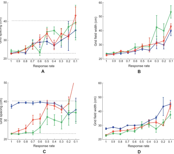
Case 11. Spectral Spacing model: Fixed rate, habituation gradient, no noise. In this case, there was a gradient in habituation rateð Þgm with the response rate fixedðmm~1Þand no noiseðsnoise~0Þ. Here, nine non-interacting cell populations, each Figure 4. Grid spacing distributions.(A, C) Data [6] and (B, D) Case 2 simulation results regarding the distribution of grid spacing at different anatomical locations along the dorsoventral axis of MEC. Panels (A) and (B) provide error bar plots of grid spacing (mean+/2SEM). In (B), blue and red curves show grid spacing of learned map cells with gridness score.0 and those with gridness score.0.3, respectively, as a function of response rateðmmÞin the last trial. The two dashed lines parallel to the x-axis in (B) signify the two potential grid scales. In (D), grid spacings derived for all model map cells are shown for each response rate. Note that map cells with gridness score.0.3 are identified by red squares, and those among the remaining with gridness score.0 by blue squares, and the rest by black squares.
with 25 category/map cells, had different habituation ratesð Þgm , with the values of 0.5, 0.2, 0.1, 0.05, 0.02, 0.01, 0.005, 0.002, and 0.001. The settings for peak activities and stripe field widths were the same as those in the response rate gradient with no noise (Case 2). Simulation results are provided in Figure 14.
Cases 12 and 13. Membrane potential oscillations: Rate gradient, fixed habituation, noise; fixed rate, habituation gradient, noise. MPOs with different periods were generated in response to a constant current input to simulate the in vitro studies of MEC layer II stellate cells at different locations on the dorsoventral axis (Figures 15A and 15A; [13,14]). Two cases were simulated, one in which the response rate varied along the dorsoventral axis with the habituation rate fixed (Case 12; Figure 15B), similar to Case 2,
and the other in which the habituation rate was varied with the response rate fixed (Case 13; Figure 15C), similar to Case 11 above. Constant current inputs of different amplitudesI~0.5, 1, 1.5, 2, and 2.5 in Equation 1.8 drove each category cell, in the absence of any intercellular interactions, for 50 s (Figure 16). Cellular noise ðsnoise~0:05Þ was added to help
unmask damped oscillations [59].
Results
Effects of different response rates on individual cells Figure 3 shows the results of the single cell simulation of Case 1 when that cell is given different response ratesmmin Equation 1.5 in response to a stripe cell-like input (Figure 3A). Figure 3B shows
Figure 5. Grid field width distributions.(A, C) Data [6] and (B, D) Case 2 simulation results of the distribution of grid field width at different anatomical locations along the dorsoventral axis of MEC. Panels (A) and (B) provide error bar plots of grid field width (mean+/2SEM). In particular, panel (B) shows grid field width of learned map cells with gridness score.0 as a function of response rateðmmÞin the last trial. In (D), the width of the central peak in the spatial autocorrelogram of the rate map of all model map cells is shown for each response rate. Note that map cells with gridness score.0 are identified by blue squares, and the rest by black squares.
the cell responses Vm j {C
h iz
2
when the on-center feedback
term a Vm j h iz
2
zm
j is removed. As noted previously,
self-excitatory feedback helps to contrast-enhance cell activity (compare Figures 3B and 3F). However, if the habituative gate zm
j in Equation 1.5 is held constant at the value of one, then the
outputs perseverate through time (Figure 3C). When transmitter gating is restored, the gates respond more slowly along the dorsoventral axis as their controlling cell activities do (Figure 3D), even if the habituation rategmis the same across response rates,
due to the activity-dependent term czm
j a Vjm h iz
2!2
in
Equation 1.7. When the properties in Figures 3C and 3D are
combined multiplicatively in the on-center feedback term
a Vm j h iz
2
zm
j, it has a unimodal form that grows and decays
more slowly as the cell response ratemm is decreased along the dorsoventral axis (Figure 3E). The cell output signals
Vm j {C
h iz
2
along the axis inherit this variable-rate unimodal
form (Figure 3F). In particular, cells exhibit a temporally delayed and broader response with a smaller peak activity for lower response rates. The higher the response rate, the faster is the activation of the membrane potential, allowing the cell activity to buildup to a higher level that is then gated off as quickly by the correlated change in the effective depletion rate of the transmitter. In this way, the habituative transmitter gating mechanism plays a role akin to a slow negative current that is
Figure 6. Grid cell peak and mean firing rates.(A, C) Data [6] and (B, D) Case 2 simulations regarding the (A, B) peak rates and (C, D) mean rates of grid cells (from their smoothed spatial rate maps) at different anatomical locations along the dorsoventral axis of MEC. Error bars in each panel show SEM. Model results are derived from learned map cells with gridness score.0 in the last trial.
activated by cell activity, much like the h-currentð ÞIh [60], and
AHP currents [61].
The results of this simulation clarify how scale selection occurs (Cases 2–11). For a cell to respond with contrast-enhanced, or above-threshold, activity at any moment with the help of its self-excitatory feedback signal, its habituative transmitter needs to be at a sufficient high level. But each time the cell responds intensely, there is a collapse of the transmitter (Figure 3D), which takes longer to recover for slower response rates because of the increased duration of cell activity. This implies that, the slower the response rate, the longer the minimum temporal duration before the cell can again respond with above-threshold activity. In other words, ventral MEC cells, which have slower response rates in the model, favor periodic inputs that are presented with a longer temporal interval, and dorsal MEC cells, which have faster
response rates, favor those that are presented with a shorter temporal interval.
This property directly explains learned scale selectivity for the case of a rat running forward at a constant speed on a linear track. Then dorsal MEC cells in the model respond better to inputs at periodic positions with relatively smaller spacings, while ventral MEC cells respond better to those with relatively larger spacings. However, the situation is more complicated when the rat navigates along the type of two-dimensional real trajectory used in our simulations, for which the running speed of the rat through time varies between 0 cm/s and 146.6 cm/s with a mean of 14.03 cm/ s, a standard deviation of 9.8 cm/s, and a mean length of piecewise linear segments of only 0.9 cm. How different response rates selectively learn different spatial scales in response to such realistic trajectories is discussed in the next subsection.
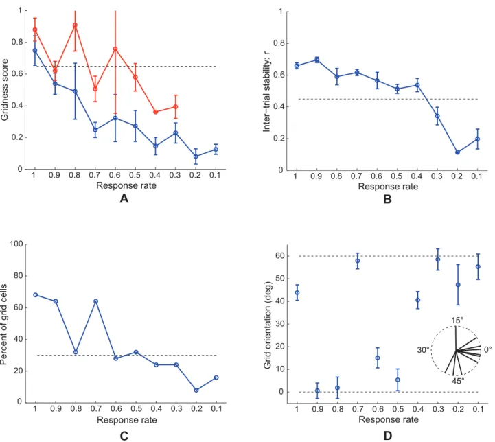
Figure 7. Case 2 results.Simulations for Case 2 of how (A) gridness score, (B) inter-trial stability, (C) percent of grid cells, and (D) grid orientation of learned map cells with gridness score.0 in the last trial vary as a function of response rateðmmÞ. Panel (A) additionally plots gridness score of learned map cells with gridness score.0.3 in the last trial (red curve). Circular mean and standard deviation for grid orientation were calculated over the range [0u, 60u). Error bars in (A), (B), and (D) depict SEM. In (D), the inset provides a polar plot to depict mean grid orientation for various response rates, with the 360u range scaled for the 60u range of orientations. The dashed lines parallel to the x-axis in (A)–(C) signify corresponding experimentally measured values for adult dorsal grid cells [37,38].
From different response rates to different learned spatial scales
Figure 4 compares neurophysiological data [6] with simulation results for Case 2 regarding the distribution of grid spacing at different anatomical locations along the dorsoventral axis of MEC. MEC grid cells exhibit periodic spatial firing fields whose spacing increases from the dorsal to the ventral ends (data: Figures 4A and 4C). Also, the spacing increases in variability along this axis. Brun and coworkers [6] remarked that the rat brain seems to allocate most of the grid cells to represent space at smaller scales, based on data that both intermediate and ventral MEC also have cells exhibiting periodic spatial responses with smaller spacings.
Emergent properties of model simulations (Figures 4B and 4D) emulate these data. Figure 4B plots grid spacing (mean+/2SEM) of learned map cells with gridness score.0 (see blue curve) and of those with gridness score .0.3 (see red curve) as a function of response rate, or equivalently the distance along dorsoventral axis,
in the last trial. Figure 4D shows the distribution of spacing of all map cells as a function of response rate. Learned map cells with gridness score.0.3 are identified by red squares, and those among the remaining with gridness score .0 are identified by blue squares, and the rest by black ones. These results indicate that, despite non-stationary variations in running speed and in heading direction along a realistic trajectory in the open field, the response rates of the map cells select the spatial scale of input stripe cells to which the learned hexagonal grid firing fields maximally respond. Faster response rates can more effectively sample smaller stripe cell spatial periods, whereas slower response rates can do the same for larger stripe cell spatial periods, for reasons that are stated more precisely in the next paragraph. In this way, faster/dorsal MEC cells learned grid fields with smaller spacings, and slower/ventral MEC cells developed preference for larger grid spacings.
As noted earlier, for each input stripe scale considered separately, the most frequent and energetic activations of grid
Figure 9. Pruned weights of inputs from multi-scale stripe cells.Simulations for Case 2 of the learned spatial fields and synaptic weights from stripe cells of two representative model grid cells, (A) one from a ventral locationðmm~0:5Þ, and (B) the other from a dorsal locationðmm~1Þ, in the last trial. The top row in each panel shows the corresponding spatial rate map and autocorrelogram, with color coding from blue (min.) to red (max.). Note the gridness score and peak firing rate on the top of the rate map, and the grid spacing on top of the autocorrelogram. And the two dashed circles centered on the central peak in the autocorrelogram signify the two potential grid scales. The bottom row in each panel provides the adapted weights from the stripe cells of the two scales (20 cm, 35 cm) to the corresponding cell. Note the solid curves trace the maximal weight from each directional group of stripe cells, the dashed lines parallel to the x-axis signify the average weight level of the projections from the corresponding scale, and the y-axes for the two spatial scales have different weight scales.
cells occur when sets of three stripe cells are coactivated whose preferred directions differ by 60u[20]. Now consider a dorsal map cell that becomes intensely active for the first time at some spatial position. During this first learning episode, the synaptic weights of its connections from stripe cells begin to get pruned to slowly match the normalized average input pattern. Given the faster dynamics of dorsal cells, this cell can again respond intensely to consistent stripe cell activations from either spatial scale at nearby positions as the animal moves around. Given the higher number of fields for a small-scale grid structure in a limited environment, and given the relatively lower peak activity of large-scale stripe cells, this dorsal cell has a higher likelihood of developing tuning to an
appropriate set of stripe cells from the small scale. On the other hand, the slower dynamics of ventral cells prevents them, on average, from developing tuning to stripe cell coactivations from the small scale, because they tend to recur faster than the recovery rate of the ventral habituative transmitters. As a result, ventral cells that develop grid-like spatial selectivity gradually prefer stripe cell coactivations from the large scale. Increased variability in grid spacing for ventral cells may be understood as a manifestation of their weaker and temporally prolonged signal levels (Figure 3F), which cause broader regions of space to be incorporated into their developing selectivities. These results clarify how a gradient of temporal response rate leads to selective learning of the gradient of
Figure 10. Spatial learning dynamics of two example model cells.Case 2 simulations showing the learned spatial fields of two representative model cells, (A) one from a ventral locationðmm~0:5Þ, and (B) the other from a dorsal locationðmm~1Þ, across the learning trials. The top and bottom row in each panel show the corresponding spatial rate map and autocorrelogram, respectively. Color coding from blue (min.) to red (max.) is used for these. Note the trial number (e.g., T1 = trial 1) and gridness score on top of each rate map, and grid spacing on top of each associated autocorrelogram.
grid spatial scale, and are thus consistent with a recent study using HCN1 knockout mice regarding how manipulation of the anatomical gradient in intrinsic properties of stellate cells affects the gradient in grid scale [62].
Figure 5 shows neurophysiological data [6] and simulation results for Case 2 regarding the distribution of grid field width at different anatomical locations along the dorsoventral axis of MEC. MEC cells exhibit periodic spatial firing fields whose width increases from the dorsal to the ventral ends (data: Figures 5A and 5C). As for grid spacing, the grid field width also increases in variability along the axis. Model simulations (Figures 5B and 5D) match these data. An estimate for grid field width was obtained by computing the width of the central peak in the autocorrelogram where the correlation crosses zero. Figure 5B plots grid field width (mean+/2SEM) of learned grid cells as a function of response rate, or the distance along the dorsoventral axis, in the last trial. Figure 5D shows the distribution of field width of all map cells as a function of response rate. Learned grid cells are identified by red squares, while others by black ones.
Decrease of peak firing rate along the gradient
Figure 6 shows neurophysiological data [6] and simulation results for Case 2 regarding the peak and mean firing rates of grid cells at different anatomical locations along the dorsoventral axis of MEC. Unlike grid spacing and grid field width, thepeakfiring rate of MEC cells decreases from the dorsal to the ventral ends (data: Figure 6A). There is also a negative trend formeanfiring rate along the axis (data: Figure 6C). The model simulates and explains these data too by using the response rate gradient and normalized grid cell receptive fields, respectively. Figures 6B and 6D plot (mean +/2 SEM) peak and mean firing rates, respectively, of learned grid cells as a function of response rate, or the distance along the dorsoventral axis, in the last trial. As we have already seen, faster response rates of map cells result in higher peak output activities (see Figure 3F). Given that the total area of the grid firing fields is roughly constant, or normalized, across spatial scales, a decrease in peak firing rate along the dorsoventral axis explains a decrease in mean firing rate.
Multiple learned cell properties match neurophysiological grid cell data
Figure 7 shows how (A) gridness score, (B) inter-trial stability, (C) percent, and (D) grid orientation of learned grid cells in the last trial vary as a function of response rate for Case 2. Error bar plots (mean+/2SEM) are shown for gridness score, inter-trial stability, and grid orientation. Due to the regular hexagonal structure of grid cell spatial fields, grid orientation varies between 0uand 60u. Moreover, since grid orientations of 0u and 60u are identical, circular mean and standard deviation were calculated over the range of [0u, 60u). The hexagonal and periodic quality of the learned spatial firing fields, measured by the gridness score, decreases with response rate. Similarly, the spatial stability of the learned grid-like firing fields between consecutive trials, called the inter-trial stability, tends to decrease for slower response rates, with
relatively poorer stability for the most ventral of the model MEC cells. The decrease in gridness score with distance along the model’s dorsoventral axis coincides with the decrease in the proportion of learned grid cells. These three simulation results together suggest poorer and less stable pattern learning for ventral cells. Given the temporally delayed and broader output responses of ventral cells, the periods when the postsynaptic learning gate
Vm j {C
h iz
2
in Equation 1.6 is positive do not correlate
temporally as well with the activities of the triggering coactive stripe cells; compare the black curve in Figure 3A with the blue curve in Figure 3F. This situation results in a persistent recoding of the incoming weights for ventral cells as the trajectory is traversed, explaining their weaker inter-trial stability and gridness score measures. Fyhn and colleagues [3] have reported consistent data showing lower spatial stability for cells in ventromedial MEC compared to dorsolateral MEC (see their Figure 4J), but the recording enclosures used were relatively small to appropriately sample the large spatial scale of the ventral cells.
Model grid cells in each of the MEC local populations along the dorsoventral axis did not learn exactly the same grid orientation. However, given the recurrent inhibition among the category cells, the different hexagonal grid fields that are learned as a result of self-organization have minimal overlap among them, because of which all possible grid orientations are not equally likely. This can be understood as a consequence of how two sets of hexagonal grid fields of the same scale can have the least total overlap only when they share the same orientation. In SOM model simulations, clustering around a dominant orientation is often observed [20]. This occurs despite the lack of excitatory coupling among neighboring category cells, which helps to prevent a topographic map of grid spatial phases from being learned (data: [5]). Existing data on grid orientation at various dorsoventral locations are preliminary (Figure 2e in [5]; Supplementary Figure 4 in [63]), but seem to suggest a narrowly tuned distribution for grid cells recorded on the same tetrode. In our simulations, we observed that in general the spread of the orientation distribution is inversely correlated with the number of learned grid cells in the local population (see Figure 11H below for an example of a narrow learned orientation distribution). More systematic work aimed at ascertaining how the mean and spread of the grid orientation distribution vary along the dorsoventral axis is needed. The learned mean grid orientations along the response rate gradient, for Case 2, have a circular standard deviation of 9.87u, suggesting that grid orientations of different scales may not be similar. This is expected as the different local populations in our model do not mutually interact. The standard deviation of learned mean grid orientations for various response rates was 12.05u when a novel trajectory was used in each trial (see Figure 11G below), and was 12.76u when three input stripe cell spatial scales (20, 35, and 50 cm) were employed (see Figure 12F below).
Figure 8 presents simulation results for Case 2 regarding how various measures of learned grid cells vary as a function of number of learning trials, for two representative response rates (dorsal:
Figure 11. Case 3 results.Case 3 simulations in which the model animal runs along a novel realistic trajectory in each trial. TheSimulation Settingssubsection in theMethodssection describes how various novel trajectories are generated from one realistic rat trajectory. Several measures of learned map cells with gridness score.0 in the last trial are shown as a function of response rateðmmÞ: (A) grid spacing, (B) grid field width, (C) gridness score, (D) inter-trial stability, (E) percent of grid cells, (F) peak rate, and (G) grid orientation. Panel (H) shows the grid orientation distribution of map cells with gridness score.0 in the last trial for the dorsal most MEC populationðmm~1Þ. In (A) and (C), the red curves plot the corresponding measures of map cells with gridness score.0.3 in the last trial. The two dashed lines parallel to the x-axis in (A) signify the two potential grid scales. Dashed lines parallel to the x-axis in (C)–(E) signify experimentally measured values for adult dorsal grid cells [37,38]. Error bars, present in all panels but (E) and (H) show SEM.
Figure 12. Case 4 results.Case 4 simulations in which the category cells receive projections from input stripe cells of three spacings (20 cm, 35 cm, and 50 cm). Several measures of learned map cells with gridness score.0 in the last trial are shown as a function of response rateðmmÞ: (A) grid spacing, (B) grid field width, (C) gridness score, (D) inter-trial stability, (E) percent of grid cells, and (F) grid orientation. In (A) and (C), the red curves plot the corresponding measures of map cells with gridness score.0.3 in the last trial. The three dashed lines parallel to the x-axis in (A) signify the three potential grid scales. Dashed lines parallel to the x-axis in (C)–(E) signify experimentally measured values for adult dorsal grid cells [37,38]. Error bars, present in all panels but (E) show SEM.
mm~1; ventral:mm~0:5). Reported measures are (A) grid spacing, (B) grid field width, (C) gridness score, and (D) inter-trial stability. Despite having to learn in response to two input stripe spatial scales, dorsal MEC cells (green curves in the four panels) pick out their spatial scale (grid spacing, grid field width) quickly and do not change their preference through time (Figure 8A). There is not much change in the inter-trial stability measure either (Figure 8D). Average hexagonal gridness quality of the learned grid firing fields for these model dorsal cells, however, shows gradual improvement over trials (Figure 8C). This is consistent with developmental data from rat pups regarding how emerging grid cells show significantly more change (improvement) in gridness score than in grid spacing [37]. Both the gradual improvement in gridness score of the grid cells with faster rates (Figure 8C, green curve) and the more rapid selection of grid spatial scales (separable curves in Figures 8A and 8B) reflect the tuning of bottom-up weights from stripe cells to grid cells. The rapid separation during learning of fast and slow rate
grid cell properties can occur as soon as the different rates preferentially select stripe cells of compatible scale. The more gradual development of the gridness score for the faster response cells requires, in addition, detection and selection of the subset of projections from stripe cells of the smaller scale that are most frequently and energetically coactivated, and the suppression of less favorable correlations.
The ventral MEC cells (blue curves in the four panels) exhibit lower gridness scores (Figure 8C) and inter-trial stability (Figure 8D) measures that do change much through time, but show more fluctuation in their spatial measures through time (Figures 8A and 8B), although they exhibit higher values overall. As we have already discussed above, the slower dynamics of ventral cells explains their poorer learning and lower stability. The variability through time of their spatial scale may also be related to their energetically smaller and temporally broader signal levels (Figure 3F).
Figure 13. Results for Cases 5–10.(A, C) Grid spacing and (B, D) grid field width of learned map cells with gridness score.0 in the last trial as a function of response rateðmmÞfor different model and input variations: Case 5 (red curves in (A) and (B)); Case 6 (blue curves in (A) and (B)); Case 7 (green curves in (A) and (B)); Case 8 (blue curves in (C) and (D)); Case 9 (green curves in (C) and (D)); and Case 10 (red curves in (C) and (D)). See the Simulation Settingsfor detailed description of these various cases. The two dashed lines parallel to the x-axis in (A) and (C) signify the two potential grid scales. Error bars in each panel depict SEM.
Figure 14. Case 11 results.Simulations for Case 11 in which it is the habituation rate that is varied with distance along the dorsoventral axis of MEC. Several measures of learned map cells with gridness score.0 in the last trial are shown as a function of habituation rateð Þgm: (A) grid spacing, (B) grid field width, (C) gridness score, (D) inter-trial stability, (E) percent of grid cells, and (F) peak rate. In (A) and (C), the red curves plot the corresponding measures for map cells with gridness score.0.3 in the last trial. The two dashed lines parallel to the x-axis in (A) signify the two potential grid scales. And the dashed lines parallel to the x-axis in (C)–(E) signify experimentally measured values for adult dorsal grid cells [37,38]. Note the log10 scale of the x-axis in each panel. Error bars, present in all panels but (E), show SEM.


![Figure 4 compares neurophysiological data [6] with simulation results for Case 2 regarding the distribution of grid spacing at different anatomical locations along the dorsoventral axis of MEC.](https://thumb-eu.123doks.com/thumbv2/123dok_br/18186390.331783/15.918.99.809.84.738/neurophysiological-simulation-regarding-distribution-different-anatomical-locations-dorsoventral.webp)