A global carbon assimilation system based on a dual optimization method

(1)

BGD

11, 14269–14317, 2014

A global carbon assimilation system

based on a dual optimization method

H. Zheng et al.

Title Page

Abstract Introduction

Conclusions References

Tables Figures

◭ ◮

Back Close

Full Screen / Esc

Printer-friendly Version

Interactive Discussion

Discussion

P

a

per

|

Discus

sion

P

a

per

|

Discussion

P

a

per

|

Discussion

P

a

per

|

Biogeosciences Discuss., 11, 14269–14317, 2014 www.biogeosciences-discuss.net/11/14269/2014/ doi:10.5194/bgd-11-14269-2014

This discussion paper is/has been under review for the journal Biogeosciences (BG). Please refer to the corresponding final paper in BG if available.

A global carbon assimilation system

based on a dual optimization method

H. Zheng1, Y. Li1, J. M. Chen2,3, T. Wang4, Q. Huang1, W. X. Huang1, S. M. Li1, W. P. Yuan5, X. Zheng5, S. P. Zhang5, Z. Q. Chen5, and F. Jiang3

1

Department of Statistics, School of Mathematical Sciences, Beijing Normal University, Beijing 100875, China

2

Department of Geography and Program in Planning, University of Toronto, Toronto M5S 3G3, Canada

3

International Institute of Earth System Science, Nanjing University, Nanjing 210093, China

4

Department of Mathematics and Statistics, University of Otago, Dunedin 9016, New Zealand

5

College of Global Change and Earth System Science, Beijing Normal University, Beijing 100875, China

Received: 28 August 2014 – Accepted: 12 September 2014 – Published: 2 October 2014

Correspondence to: Y. Li ([email protected]) and J. M. Chen ([email protected])

(2)

BGD

11, 14269–14317, 2014

H. Zheng et al.

Title Page

Tables Figures

◭ ◮

Back Close

Full Screen / Esc

Discussion

P

a

per

|

Discus

sion

P

a

per

|

Discussion

P

a

per

|

Discussion

P

a

per

Abstract

Ecological models are effective tools to simulate the distribution of global carbon sources and sinks. However, these models often suffer from substantial biases due to inaccurate simulations of complex ecological processes. We introduce a set of scaling factors (parameters) to an ecological model on the basis of plant functional 5

type (PFT) and latitudes. A global carbon assimilation system (GCAS-DOM) is devel-oped by employing a Dual Optimization Method (DOM) to invert the time-dependent ecological model parameter state and the net carbon flux state simultaneously. We use GCAS-DOM to estimate the global distribution of the CO2 flux on 1◦×1◦ grid

cells for the period from 2000 to 2007. Results show that land and ocean absorb 10

−3.69±0.49 Pg C year−1 and −1.91±0.16 Pg C year−1, respectively. North America, Europe and China contribut −0.96±0.15 Pg C year−1, −0.42±0.08 Pg C year−1 and −0.21±0.28 Pg C year−1, respectively. The uncertainties in the flux after optimization by GCAS-DOM have been remarkably reduced by more than 60 %. Through parameter optimization, GCAS-DOM can provide improved estimates of the carbon flux for each 15

PFT. Coniferous forest (−0.97±0.27 Pg C year−1) is the largest contributor to the global carbon sink. Fluxes of once-dominant deciduous forest generated by BEPS is reduced to−0.79±0.22 Pg C year−1, being the third largest carbon sink.

1 Introduction

The spatiotemporal distribution of carbon sources and sinks has drawn much atten-20

(3)

BGD

11, 14269–14317, 2014

H. Zheng et al.

Title Page

Tables Figures

◭ ◮

Back Close

Full Screen / Esc

Discussion

P

a

per

|

Discus

sion

P

a

per

|

Discussion

P

a

per

|

Discussion

P

a

per

|

Atmospheric inversion uses CO₂ observations to infer the distribution of the carbon flux from global (Patra et al., 2005; Rödenbeck, 2005; Rayner et al., 2008; Maki et al., 2010) to regional scales (Gerbig et al., 2003; Peylin et al., 2005; Peters et al., 2007; Schuh et al., 2010). It involves an atmospheric transport model to link the measured CO2concentration in the atmosphere to the surface CO2flux. However, the

measure-5

ments from sparsely located observational sites are not sufficient for estimating global carbon sources and sinks in fine grids. Enting (1995, 2002) suggested to use a prior flux to regularize the inverted flux based on the Bayesian synthesis inversion method (BSIM). The posterior flux is determined by minimizing the difference between simu-lated and observed concentrations and between posterior and prior fluxes.

10

In BSIM, the prior information is normally precalculated from an ecological model, e.g., Carnegie-Ames-Stanford Approach (CASA) Biosphere model (Gurney et al., 2003, 2004; Baker et al., 2006), and Boreal Ecosystems Productivity Simulator (BEPS) model (Deng et al., 2007; Deng and Chen, 2011). These process-based models are constructed to estimate carbon sources and sinks based on the mechanisms of photo-15

synthesis, autotrophic respiration, organic matter decomposition and nutrient cycling. However, their estimates of carbon sources and sinks at regional scales often have substantial biases, and the purpose of atmospheric inversion is to reduce these biases using the additional information of atmospheric CO2concentration. Atmospheric

inver-sion methods di_ffer considerably in the inverted carbon flux distribution among large 20

regions of the globe (Peylin et al., 2013), and therefore improvements are still needed in the prior flux estimation and the optimization using atmospheric CO2data.

In consideration of the possible biases in the prior flux produced by an ecological model, scaling factors are introduced to the prior flux to correct the biases (Peters et al., 2007, 2010; Zupanski et al., 2007; Lokupitiya et al., 2008; Schuh et al., 2010). 25

(4)

Pe-BGD

11, 14269–14317, 2014

H. Zheng et al.

Title Page

Tables Figures

◭ ◮

Back Close

Full Screen / Esc

Discussion

P

a

per

|

Discus

sion

P

a

per

|

Discussion

P

a

per

|

Discussion

P

a

per

ters et al. (2007, 2010) considered a more complex forecast model which combines the information of biases in two steps before the current time step. An Ensemble Kalman Filter (Evensen, 2007) is often used for estimating the unknown scaling factors and the posterior flux is the prior flux scaled by the estimated scaling factors. This ensemble-based assimilation method takes relatively long time to warm the system to reach a sta-5

ble estimation of these scaling factors, and the filtering divergence (e.g., Houtekamer and Mitchell, 1998) that retards the converge of the estimate towards observations is still a problem.

Zheng et al. (2013) proposed a dual optimization method (DOM) to estimate both the scaling factors (hereinafter known as parameters) of an ecological model and gridded 10

carbon fluxes. DOM introduces a scaled ecological model designed by plant functional types (PFTs), and uses CO2 observations to invert the unknown states of the

param-eters and net flux simultaneously. DOM is an objective method which depends just on the information of concentration observations and the structure of the ecological model, but no forecast model is needed. The estimation precision of fluxes can be greatly im-15

proved by the dual optimization, and the statistical properties of parameters and fluxes also provide useful information about the inversion accuracy.

As DOM inverts the flux for all regions and all times simultaneously using all ob-servations at the same time, it requires much computational resources. Therefore, it is inconceivable to use DOM to estimate the global distribution of the carbon flux at 20

high spatial and temporal resolutions. In this study, a moving-window method similar to that of Bruhwiler et al. (2005) is developed. Different from a batch model which uses all observations to invert fluxes for all source regions at all times simultaneously, Bruh-wiler et al. (2005) adopted a temporal moving window and used the CO2concentration

observations at the current time (the end of the window) to estimate carbon fluxes in 25

(5)

BGD

11, 14269–14317, 2014

H. Zheng et al.

Title Page

Tables Figures

◭ ◮

Back Close

Full Screen / Esc

Discussion

P

a

per

|

Discus

sion

P

a

per

|

Discussion

P

a

per

|

Discussion

P

a

per

|

Due to the difference of seasonal and meteorological conditions at different latitudes, we redesign the scaling factors by dividing the globe into several latitudinal zones. Each zone shares a set of scaling factors. The number of parameters assigned to each grid equals the number of PFTs in the grid so that one parameter is associated with one PFT. This is different from Carbon Tracker (Peters et al., 2007, 2010) in which each grid is assigned to one category based on the dominant vegetation type. On the basis 5

of the above settings, we build a global carbon assimilation system (GCAS-DOM) by combining DOM with an atmospheric transport model (MOZART-4). The forecast of the assimilation system is embodied in updating the background concentration field. At each step, the background CO₂ concentration is updated by running MOZART-4 for-ward forced with the optimized flux at the last step. Finally we use the GCAS-DOM to 10

estimate the worldwide weekly flux in 1◦×1◦grid for a relatively long period of 8 years. Results show its accuracy in flux estimation and significant effect in uncertainty reduc-tion.

The objectives of this study are: (1) to develop a global carbon assimilation system using DOM, i.e. GCAS-DOM for the purpose of improving the estimation of the global 15

distribution of the carbon flux, (2) to produce with GCAS-DOM a global carbon flux field on 1◦×1◦ grid cells from 2000 to 2007 and analyze the flux in terms of its long-term mean, and interannual variations for the globe and selected large regions; and (3) to investigate the impacts of atmospheric CO₂data on the estimation of the carbon flux per PFT for the evaluation of ecosystem models. This paper is organized as follows. 20

Section 2 consists of detailed descriptions on each component of the GCAS-DOM. It begins with the introduction of state variables in Sect. 2.1. Then in Sect. 2.2, we will show the procedure of building the GCAS-DOM by using a moving-window method. Section 2.3 presents the estimation method of state variables in a window. The calcu-lation of the uncertainties is given in Sect. 2.4. In Sect. 3, we conduct an application 25

(6)

BGD

11, 14269–14317, 2014

H. Zheng et al.

Title Page

Tables Figures

◭ ◮

Back Close

Full Screen / Esc

Discussion

P

a

per

|

Discus

sion

P

a

per

|

Discussion

P

a

per

|

Discussion

P

a

per

2 Methodology

GCAS-DOM consists of three major components: an ecological model and an atmo-spheric transport model, a moving window and the optimization module. The ecologi-5

cal model provides the first guess of the flux before data assimilation. The atmospheric transport model links the flux to the CO2 mixing concentration ratio. Considering the

computational feasibility, we use a temporal moving window in which the flux is opti-mized using the optimization algorithm DOM.

2.1 State Variables

10

The ecosystem model is formed to simulate the variations of carbon sources and sinks based on the mechanism of carbon cycling. As improperly simulated ecological pro-cesses could result in biases in the flux, we consider a scaled ecosystem model similar to that of Lokupitiya et al. (2008). But different from Lokupitiya et al. (2008), which ad-justs ecosystem respiration (ER) and gross primary productivity (GPP) using separate 15

scaling factors, only the net ecosystem exchange (NEE) defined as the difference be-tween ER and GPP is scaled because ER is strongly associated with GPP and both of them are much larger than the ocean flux in magnitude. Hence the parametric model can be represented as

s=λNEE·sNEE+λOCE·sOCE+sFF+sFIRE+ε (1)

20

wheres_OCE is the first-guess ocean flux computed from an ocean exchange model;

sNEE is the first-guess biospheric flux estimated from a terrestrial ecosystem model;

sFFandsFIREare fossil fuel and fire fluxes estimated from inventory-based emissions;

λ_NEE and λ_OCE are sets of scaling factors applied to land surface fluxes and ocean 25

(7)

BGD

11, 14269–14317, 2014

H. Zheng et al.

Title Page Abstract Introduction Conclusions References Tables Figures ◭ ◮ ◭ ◮ Back Close

Full Screen / Esc

Printer-friendly Version Interactive Discussion Discussion P a per | Discus sion P a per | Discussion P a per | Discussion P a per |

Zheng et al. (2013) suggests to specify the structure of parameters according to PFT to avoid over-adjustment or excessive computation. In consideration of the fact that (1) the seasonal variation in climate in the North Pole is opposite to that in the South Pole, 5

and (2) the tropical rainforest has high temperature all year around, it is not effective to specify parameter states just according to PFT. In this study, we divide the globe intoq

zones according to latitude and assume that the vegetation distribution is mapped onto

pPFTs. Thus a grid box can contain up top₊1 different types (pPFTs and 1 oceanic type) quantified with an areal fraction for each PFT in the grid.

10

We decompose the flux in each grid box intop₊1 components with each denoting the flux generated from one PFT. To facilitate the expression, we usesm,j for the gridded flux in thejth latitude zone computed from land and oceanic models, and it is denoted as follows

sm,j =sj_OCE sj_NEE,1 s_NEE,2j · · · sj_NEE,_p, j₌1, 2,. . .,q (2)

15

wheresj_OCE is a vector for the oceanic component and sj_NEE,_i is a vector for the ter-restrial component for theith PFT. Gridded fluxes at the same latitude zone share the same set of parameters and thus the corresponding parameter for thesm,j is

λj=λj_OCE λ_NEE,1j λj_NEE,2 · · · λj_NEE,_p

T

, 20

where each element is a scaler used to scale the corresponding column vector ofsm,j. Then model (1) can be rewritten as

s=     

sm,1 sm,2

. ..

sm,q

          λ1 λ2 .. . λq     

+sFF+sFIRE+ε

,_sm_λ

+s_FF₊s_FIRE₊ε.

(8)

BGD

11, 14269–14317, 2014

H. Zheng et al.

Title Page

Tables Figures

◭ ◮

Back Close

Full Screen / Esc

Discussion

P

a

per

|

Discus

sion

P

a

per

|

Discussion

P

a

per

|

Discussion

P

a

per

wheresm, referred to the prior flux, is the reshaped form of the flux computed from 5

the ecosystem model in the order of latitude, andλ= λ1T λ2T · · · λqT

T

is a set of scaling factors;ε is the model error with zero mean and covariance matrix Q. In Model (3), as sFF and sFire are imposed without optimization, their contributions to

concentration can be subtracted from the observation concentrations directly. Then model (3) can be expressed in a simplified expression:

10

s=smλ+ε. (4)

2.2 Time-stepping

In the application of GCAS-DOM, one of the major difficulties in estimating the carbon flux is the computational cost at high resolution. To overcome this difficulty, we adopt 15

a method similar to that of Bruhwiler et al. (2005). At each time t, we use the obser-vations of CO2 concentration and the carbon flux in the time window betweent and

t₊l−1, where l is window length which could be in days, weeks, or months. This is different from Bruhwiler et al. (2005) where only the observations at timet₊l−1 are used. We therefore have a (t,l)-window, which uses the CO2 concentration

observa-20

tions{ct+k, 0≤k≤l−1}and the carbon flux{st+k, 0≤k≤l−1}at each time pointt,

where the column vectorc_t₊_k represents the observed CO₂ mixing ratios of a given site att₊k, and the column vectorst+kis the global carbon flux in the time period from

t₊k−1 tot₊k.

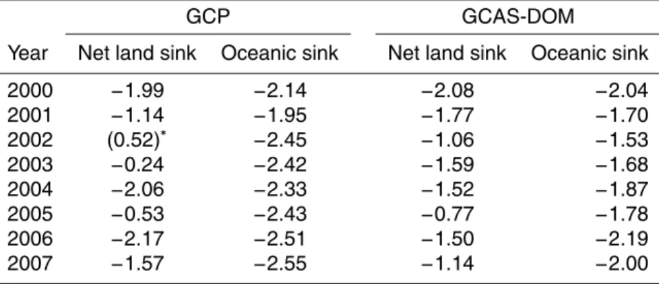
The time stepping in the assimilation scheme is illustrated in Fig. 1. The light shaded 25

boxes represent the the prior flux at each step computed by the ecosystem model. The dark shaded boxes stand for the optimized flux. We now describe one cycle of GCAS-DOM. The first step is to use the background CO₂ concentration C(t−1) as the initial value, which is a 3-D matrix for the spatial distribution of CO2concentration

(9)

BGD

11, 14269–14317, 2014

H. Zheng et al.

Title Page

Tables Figures

◭ ◮

Back Close

Full Screen / Esc

Discussion

P

a

per

|

Discus

sion

P

a

per

|

Discussion

P

a

per

|

Discussion

P

a

per

|

all times in this window which gives{C(t),. . .,C(t₊l−1)}and extract CO₂mixing ratios 5

at observation sites as{cb_t,. . .,cb_t₊_l₋₁}. The second step is to estimate the optimized fluxes{sˆt+k, 0≤k≤l−1}using the resulting mixing ratios at sites{c

b t,. . .,c

b

t+l−1}, the

observations of CO₂ concentrations in the window {c_t,. . .,c_t₊_l₋₁}, and the prior flux in the window {sm_t₊_k, 0≤k≤l−1}. The estimation method is introduced in the next section. The optimized flux ˆst does not need to be estimated in the next cycle and

10

is therefore used as an estimate of the flux at time t. In the third step, we run the transport model one step forward starting fromC(t−1) forced with the optimized flux

ˆ

stto get the updated spatial distribution of concentrationC′(t). Then we use observed

CO₂concentration to assimilate theC′(t) instead of directly using it as the background concentration at timetfor the next cycle in previous studies. We extract updated CO2

15

concentration at locations of CO2observation sits from theC′(t) and compare it to the

observed concentrationc_t at time t. A constant adjustment, which is computed from the site-averaged difference between the above two vectors, is imposed onC′(t) to get an optimized spatial patternC(t) at timet.1In the forth step, we move the window one step forward so a new fluxsm_t₊_l and a new concentration observation c_t₊_l are read in 20

to the system for the next computational cycle, which begins from background CO2

concentrationC(t).

2.3 Adaptive DOM

In this section, we introduce the method for estimating parameters and the carbon flux in a window. Zheng et al. (2013) proposed a DOM to improve the accuracy of the 25

optimized flux and successfully applied it to the inversion of the flux for the globe divided into 50 regions. In this study, we expect to use DOM in each (t,l)-window. As the fluxes computed for different PFTs are often correlated, direct application of the DOM to flux inversion at a high resolution will result in many abnormal estimators of parameters and

1

(10)

BGD

11, 14269–14317, 2014

H. Zheng et al.

Title Page

Tables Figures

◭ ◮

Back Close

Full Screen / Esc

Discussion

P

a

per

|

Discus

sion

P

a

per

|

Discussion

P

a

per

|

Discussion

P

a

per

large uncertainties of both parameters and fluxes. Therefore, we propose an adaptive 5

version of DOM by adding additional regularization of scale factors which is referred to as a stochastically constrained equation (Theil and Goldberger, 1961)

λ=1₊ζ, (5)

where1 is a vector with all elements equaling to 1 and ζ is the random error of the 10

regularization withE(ζ)=0, and the dispersion matrix var(ζ)=W.

Then we will present the adaptive DOM in a (t,l)-window. To facilitate the discussion, we first introduce two denotations: (1) the observations of CO₂ concentration in (t,l )-window is denoted by a vector

c(t,l)=cT_t cT_t₊₁ · · · cT_t₊_l₋₁

T

, (6)

15

and named as the (t,l)-window observation concentration, (2) the flux is denoted as

s(t,l)=sT_t sT_t₊₁ · · · sT_t₊_l₋₁

T

(7)

and named as the (t,l)-window flux. 20

The (t,l)-window observation concentration c(t,l) contains information from two sources, the (t,l)-window flux s(t,l) and concentration transported from the previous time stepC(t−1). We letcw(t,l)be the CO₂concentration determined bys(t,l), and re-fer it as (t,l)-window flux concentration. In fact,cw(t,l)is the difference between window observation concentrationc(t,l) and{cb_t,. . .,cb_t₊_l₋₁}(mentioned in Sect. 2.2). Then the

cw(t,l)follows that

cw(t,l)=G(t,l)s(t,l)+η(t,l), (8)

(11)

BGD

11, 14269–14317, 2014

H. Zheng et al.

Title Page

Tables Figures

◭ ◮

Back Close

Full Screen / Esc

Discussion

P

a

per

|

Discus

sion

P

a

per

|

Discussion

P

a

per

|

Discussion

P

a

per

|

whereε(t,l) is the error of window concentration observation, and

G(t,l)=



   

G_t,t

G_t₊_1,_t G_t₊_1,_t₊₁

..

. ... . ..

G_t₊_l₋_1,_t G_t₊_l₋_1,_t₊₁ · · · G_t₊_l₋_1,_t₊_l₋₁



   

(9)

is the (t,l)-window atmospheric transport matrix. It describes the contribution of the 10

window flux to the observation sites. Each submatrixG_m_,_n represents the influence of the flux (normalized to 1 g C) at timenon the concentration at observation sites at time

m.

In a (t,l)-window, we minimize the following objective function (10) to obtain the optimized (t,l)-window flux. This function is similar to that of DOM but with an extra 15

penalty term, so it is called the adaptive DOM. To simplify the expression, all subscripts (t,l) are omitted here.

J(s,λ)=(Gs−cw)TR−1(Gs−cw)+(s−smλ)TQ−1(s−smλ)

+(λ−1)TW−1(λ−1) (10)

20

wheresm=diag sm_t ,. . .,sm_t₊_l₋₁

is the prior fluxes for the (t,l) window,Qis the error covariance matrix of the corresponding prior fluxes,Ris the covariance matrix of the window concentration observation errorη, andWis the variance of constrained error.

Solving for the minimum of cost function (10) with respect tosandλis similar to the process in DOM. The solutions are given by the following two equations (see Appendix A for details)

( ˆ

λ=(XTΣX+W−1)−1(XTΣcw+W−11) ˆ

s=QGTΣ(cw−Gsmλˆ)+smλˆ (11)

(12)

BGD

11, 14269–14317, 2014

H. Zheng et al.

Title Page

Tables Figures

◭ ◮

Back Close

Full Screen / Esc

Discussion

P

a

per

|

Discus

sion

P

a

per

|

Discussion

P

a

per

|

Discussion

P

a

per

whereΣ=(R₊GQGT)−1,X₌Gsmand ˆs₌sˆT_t sˆT_t₊₁ · · · sˆT_t₊_l₋₁ T

. As the estimation of ˆstuses the most amount of observations, it has the highest accuracy. We therefore

use ˆstas the optimized carbon flux at timet.

2.4 Calculation of uncertainty

10

The estimators given by Eq. (11) have the following uncertainties (see Appendix A for details):

(

var( ˆλ)=(XTΣX₊W−1)−1

var( ˆs)=QGTΣ(I−Xvar( ˆλ)XTΣ)GQ+smvar( ˆλ)(sm)T (12)

Note that the uncertainty of the parameter estimator is incorporated into the variance 15

of estimated fluxes.

3 Application

In this section, we use the GCAS-DOM to estimate the weekly carbon flux from 2000 to 2007 on 1◦×1◦global grid cells.

3.1 Ecological model

20

(13)

BGD

11, 14269–14317, 2014

H. Zheng et al.

Title Page

Tables Figures

◭ ◮

Back Close

Full Screen / Esc

Discussion

P

a

per

|

Discus

sion

P

a

per

|

Discussion

P

a

per

|

Discussion

P

a

per

|

fluxes is modeled by BEPS at the resolution 1◦×1◦. The oceanic flux at 1◦×1◦ spa-5

tial resolution is obtained from Carbon Tracker 2010 (CT20102) results (available via http://www.esrl.noaa.gov/gmd/ccgg/carbontracker/download.html).

In BEPS, vegetation is mapped onto 6 PFTs including coniferous forest, deciduous forest, evergreen forest, shrub land, C4 vegetation and “other vegetation”. A grid cell can contain up to 7 different cover types (6PFTs+1 ocean type) with their correspond-10

ing coverage fraction. We divide equally the globe excluding China into 30 zones by latitude and each spreads a range of 6◦. China is separately split into 6 zones and each spreads a range of 6◦as well. Thus we yield a total of 30+6=36 zones (see Fig. 2). In each latitude zone, there are six PFTs and 1 ocean type. As PFTs vary slowly in a short time, we assume that they are time independent within a window. Thus, we 15

have 7×36=252 parameters (1 parameter corresponds to 1 PFT in a zone) to be estimated at each time step. The model error covariance matrixQfor the prior flux is treated using the same principle in Zhang (2013) based on the theory of statistics.

The constrained matrixW(Eq. 10) for the scaling factor is defined as a diagonal ma-trix with each itemW_{i i} defining the degree of deviation from 1. The smaller the value is, 20

the closer the parameter and 1 are. Conversely, the parameter can be more influenced by other information such as CO2measurements. We use the variance of 0.01 for the

scaling factors corresponding to grids in China and 0.001 for the rest of the globe. This is because we intend optimizing the flux in China by observed concentrations to a greater extent as BEPS model might generate larger error in China.

25

3.2 Background fluxes

In the process of making inference about flux from ecosystems, we need to exclude the contribution of other CO2 fluxes such as fire and fossil fuel emissions to observed

concentrations. They are not perfectly known and but also not the target of this study. Their information is included in the observation data we use. As mentioned in Sect. 2.1,

2

(14)

BGD

11, 14269–14317, 2014

H. Zheng et al.

Title Page

Tables Figures

◭ ◮

Back Close

Full Screen / Esc

Discussion

P

a

per

|

Discus

sion

P

a

per

|

Discussion

P

a

per

|

Discussion

P

a

per

we do not include any parameters concerning fossil fuel and fire fluxes in the optimiza-tion. So the contribution of fossil fuel and fire emissions need to be extracted from the 5

window flux concentration. Then the window flux concentration excluding the influence of fire and fossil fuel is used in the process of ecosystem flux optimization.

The fossil fuel and fire fluxes are from the CT2010 results on 1◦×1◦ resolution. The annual summary of fossil fuel and fire emissions is listed in Table 1.

3.3 Atmospheric transport model

10

The carbon fluxes of the earth’s surface at a certain time affect the CO₂ concentra-tion observed in a subsequent time period in the atmosphere. Therefore, we can use the atmospheric CO2concentration to invert the historical distribution of carbon fluxes.

Atmospheric transport models are generally used to describe the process of surface fluxes spreading into the atmosphere. The commonly employed transport models in-15

clude MUGCM (Law, 1993), NCAR (Erickson et al., 1996), TM5 (Krol et al., 2005), and MOZART-4 (Emmons et al., 2010). We will use MOZART-4 in our study as its imple-mentation is flexible. MOZART-4 divides the space from the earth surface to a height of 2 hPa into 28 vertical sigma-pressure layers, and its horizontal resolution can be ad-justed according to the capacity of computers. The highest resolution by far has been 20

0.7◦×0.7◦. We use the meteorological data from the National Centers for Environ-mental Prediction (NCEP) reanalysis data (http://www.esrl.noaa.gov/psd/data/gridded/ data.ncep.reanalysis.html).

This model here is used in two forms. In its full form, the assimilation is done by running forward with the optimized flux state at the previous time step to update the 25

(15)

BGD

11, 14269–14317, 2014

H. Zheng et al.

Title Page

Tables Figures

◭ ◮

Back Close

Full Screen / Esc

Discussion

P

a

per

|

Discus

sion

P

a

per

|

Discussion

P

a

per

|

Discussion

P

a

per

|

3.4 Concentration data

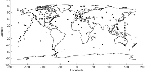
Weekly observations of CO2concentration are from GLOBALVIEW-2011 dataset (http:

5

//www.esrl.noaa.gov/gmd/ccgg/obspack/data.php). These data consist of pseudo-weekly interpolation CO₂concentration data measured at 312 global sites. The map of stations is shown in Fig. 3. As the residual standard deviations (RSD) of the CO2

con-centration data given by the var files in GLOBALVIEW-2011 dataset are in months, we convert them onto weekly value by linear interpolation, and impose a floor of 0.175 ppm 10

to the data uncertainty using the equation (Deng et al., 2007)

R=

q

(0.175 ppm)2₊_RSD2_, ₍₁₃₎

where 0.175 ppm is the system error at each site.

3.5 Window length

15

The choice of the window length is an important issue in assimilation systems. The longer a window size is, the more overlapping of transport integrations and the larger calculation demand are. However, a small window size will cause significant errors. Peters et al. (2005, 2007, 2010) used a five-week smoothing window. Here, we choose a six-week smoothing window, which is sufficiently long for the fluxes to transmit across 20

the world.

3.6 Results

(16)

BGD

11, 14269–14317, 2014

H. Zheng et al.

Title Page

Tables Figures

◭ ◮

Back Close

Full Screen / Esc

Discussion

P

a

per

|

Discus

sion

P

a

per

|

Discussion

P

a

per

|

Discussion

P

a

per

the optimized flux is shown in a map of 1◦×1◦ grid cell. We also show the fit of the optimized concentrations to the observation concentrations to evaluate the system. 5

3.6.1 Optimized parameters

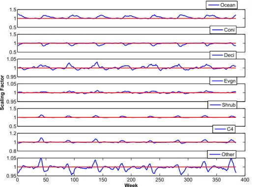
Figure 4 shows the results of the scaling factors for 6 PFTs and an oceanic type in the latitude zone spread from 24◦N to 30◦N excluding China. The estimators fluctuate around 1 with small volatility. If the value is larger than 1, it means that the absolute value of the prior flux is underestimated and therefore need to be multiplied by a factor 10

more than 1 to increase its value. On the contrary, an estimator smaller than 1 indicates a decrease of the absolute value of the flux. From the time series of weekly estimates, most of the parameters show annual periodicity and the scaling factors of coniferous type indicate opposite “swings” in contrast to other PFTs. The scaling factors of decid-uous and evergreen types have less amplitudes than those of the remaining types. 15

3.6.2 Optimized fluxes and their uncertainties

Global Carbon Budget

We compare the optimized total flux (excluding fire and fossil fuel emissions, same as thereafter) with the prior flux and the results of CT2011_oi which is a newer version of CarbonTracker released on 28 June 2013 (Fig. 5). The terrestrial fluxes make a major 20

contribution for the year 2000 to 2007 before or after optimization. Before optimization, the annual average terrestrial and oceanic fluxes are −3.16 and −1.62 Pg C year−1, respectively. GCAS-DOM increases the uptake in land and ocean by a mean value 0.52 Pg C year−1 and 0.23 Pg C year−1, respectively, over the 2000–2007. Therefore the total annual ecosystem sinks show a significant increase mainly due to the in-25

(17)

BGD

11, 14269–14317, 2014

H. Zheng et al.

Title Page

Tables Figures

◭ ◮

Back Close

Full Screen / Esc

Discussion

P

a

per

|

Discus

sion

P

a

per

|

Discussion

P

a

per

|

Discussion

P

a

per

|

are very similar. Even so, the optimized oceanic flux is still more close to the results of CT2011_oi compared to the prior flux.

The optimized result indicates that the terrestrial ecosystems and oceans respec-tively absorb an average of 3.69 and 1.85 Pg C year−1 over the 2000–2007 period. These values compare well with the inversion results of Deng and Chen (2011), which 5

are on average 3.63 and 1.84 Pg C year−1, respectively, for the years 2002–2007. We then further compare the net land sink and oceanic sink in our study to that of the Global Carbon Project (GCP, Table 2). The Global Carbon Budget 2013 v2.3 (Le Quéré et al., 2014) is the newest version released on April 2014 by the GCP. The net land sink of GCP is calculated by the difference of land sink and land-use change emissions in 10

Global Carbon Budget 2013 v2.3, while that of the GCAS-DOM is computed by the dif-ference between the terrestrial sink (Fig. 5) and fire emission in Table 1. The GCP gen-erates larger oceanic sinks than GCAS-DOM, with the smallest gap of 0.1 Pg C year−1 in 2000 and largest di_fference of 0.92 Pg C year−1 in 2002. For the net land sink, the largest difference occurs in 2002 when the GCP releases 0.52 Pg C year−1 from land 15

while the GCAS-DOM maintains a land uptake of 1.06 Pg C year−1. The 7 year mean of the net land sink excluding the year 2002 in our study is 1.48 Pg C year−1 which is close to 1.39 Pg C year−1in GCP. Figure 5 shows that the total sink in land and ocean varies considerably among years, and the variation is mostly due to the sink in land. GCAS-DOM sink results are usually larger than the prior value, indicating the prior 20

flux underestimates the land sink. The multi-year mean values of GCAS-DOM and CT2011_oi are about the same, but they differ to some extent in individual years, sug-gesting that di_fferent data assimilation methods can result in considerable di_fference in the optimized carbon flux.

From the point of inter-annual variabilities, the ocean flux shows much smaller vari-25

(18)

BGD

11, 14269–14317, 2014

H. Zheng et al.

Title Page

Tables Figures

◭ ◮

Back Close

Full Screen / Esc

Discussion

P

a

per

|

Discus

sion

P

a

per

|

Discussion

P

a

per

|

Discussion

P

a

per

in the Amazon that affects plant growth and high temperature in 2005 which intensi-fies the ecosystem respiratory activities (Deng and Chen, 2011). The relatively weak sinks in 2002 and 2007 may be related to the EI Niño Southern Oscillation event in 2002–2003 and 2006–2007, respectively, that causes anomalies in precipitation caus-ing draughts in some regions.

5

Before optimization, we use an uncertainty of 1.98 Pg C year−1for the land flux, and an uncertainty of 0.93 Pg C year−1 for the oceanic flux, resulting in a total uncertainty of 2.18 Pg C year−1 for the globe. Table 3 shows the uncertainty of optimized fluxes by GCAS-DOM. We can see different levels of uncertainty reductions for land and ocean. The uncertainty of the globe is significantly reduced by about 75–80 % and 10

ocean has the slightly larger reduction than the global value. It is mostly due to the stronger constraint by the elongated clustered observation sites over the Pacific Ocean (see Fig. 3). The uncertainty reductions of ocean and land respectively stabilize at around 82 % and 75 % for the years 2000–2007.

4 Regional Carbon Budget

15

We further analyze three large regions: Europe, North America and China. As shown in Table 4, GCAS-DOM respectively increases the sink by 0.14 Pg C year−1for Europe and 0.32 Pg C year−1 for North America compared to the prior flux for the eight-year mean. The uncertainties before optimization (0.44 Pg C year−1 and 0.86 Pg C year−1 for Europe and North America, respectively) are reduced to 0.08 Pg C year−1 and 20

0.15 Pg C year−1, respectively. The uncertainty reductions for these two regions, are remarkably large at about 80 %, possibly because the atmospheric CO2 is densely

observed in these two regions. In Europe, the carbon sink from our study (−0.42± 0.08 Pg C year−1) is higher than CT2011_oi (−0.33±1.86 Pg C year−1), Deng and Chen (2011, −0.22 Pg C year−1) and Jiang et al. (2013, −0.28±0.17 Pg C year−1). In North 25

(19)

BGD

11, 14269–14317, 2014

H. Zheng et al.

Title Page

Tables Figures

◭ ◮

Back Close

Full Screen / Esc

Discussion

P

a

per

|

Discus

sion

P

a

per

|

Discussion

P

a

per

|

Discussion

P

a

per

|

−0.81±0.21 Pg C year−1). In China, the carbon uptake slightly increases from the prior to−0.21 Pg C year−1, which is weaker than Jiang et al. (2013,−0.28±0.18 Pg C year−1) and Piao et al. (2009,−0.35±0.33 Pg C year−1). Although the change of sink in China before and after optimization is small, the uncertainty reduction is about 67 %, which is smaller than those of Europe and North America because of relatively few atmospheric 5

data observed within and around China.

The inter-annual variations of fluxes before and after optimization are shown in Fig. 6. With a minor fluctuation, the carbon uptake of Europe has an increasing trend be-fore 2004, and then decreases after 2005. Similar temporal trends are also found in North America. In the first five years, the carbon sink in China is stable around 10

−0.22 Pg C year−1, and slightly decreases from 2005 to 2007. The uncertainties of optimized fluxes for three regions vary slightly from year to year and are remarkably reduced from those of the prior fluxes.

Fluxes for each PFT

Our gridded inversion system at 1◦ resolution affords us the possibility to analyze the 15

impacts of atmospheric CO₂data on the estimation of the carbon sink by PFT. Figure 7 shows the annual mean terrestrial flux for 6 PFTs. “Prior” stands for fluxes simulated by BEPS consisting of 6 PFT components with corresponding coverage fraction in each grid, while “GCAS-DOM” represents fluxes optimized by GCAS-DOM and the statistics are based on the principle that each 1◦×1◦ gridbox is assigned to a sin-20

gle category according to the locally dominant PFT. As shown in Fig. 7, the order of the sink magnitudes of different PFTs is altered after optimization. The carbon flux of once-dominant deciduous forests is reduced from −0.96 to −0.79 Pg C year−1. After optimization, largest net uptake is shown in regions dominated by coniferous forest (−0.97±0.27 Pg C year−1) and is increased by 115.68 %. As the coniferous forest is 25

(20)

BGD

11, 14269–14317, 2014

H. Zheng et al.

Title Page

Tables Figures

◭ ◮

Back Close

Full Screen / Esc

Discussion

P

a

per

|

Discus

sion

P

a

per

|

Discussion

P

a

per

|

Discussion

P

a

per

increase in the sink magnitude for conifer from the prior estimate suggests that the ecosystem model considerably underestimates the sink for this PFT. “Other vegeta-tion” (−0.86±0.20 Pg C year−1) and deciduous forest (−0.79±0.22 Pg C year−1) are re-spectively the second and third PFTs in terms of their total sink magnitude. Evergreen forests most located in the Southern Hemisphere absorb−0.77±0.21 Pg C year−1on 5

average. Relatively speaking, shrub land (−0.17±0.12 Pg C year−1) and C4 vegetation (−0.26±0.13 Pg C year−1) make the least contributions to the total global carbon sink. The slight changes in the sink magnitudes of Shrub land and C4 vegetation before and after optimization suggest that BEPS provides nearly unbiased sink estimates for these two PFTs. The sink magnitude of the “other vegetation” is modified greatly by optimiza-10

tion, suggesting BEPS does not work well for all other land cover types lumped into this PFT. One way to improve BEPS would be to introduce more PFTs. Through this analysis, we show that GCAS-DOM has provided a useful model framework to eval-uate an ecosystem model by PFT, and it can potentially provide directions for further development of ecosystem models.

15

To further investigate the seasonal variation of the carbon flux, we compare the op-timized weekly fluxes to the prior fluxes by PFT. For this purpose, we select the results of coniferous forest and “other vegetation” (Figs. 8 and 9), as fluxes by these two types present largest change after optimization among all PFTs. All the time series exhibit pronounced seasonality, and Northern Hemisphere and Southern Hemisphere show 20

opposite seasonal patterns. In Northern Hemisphere, the optimized flux of coniferous forest shows a general shift towards larger sinks in all seasons from that of the prior flux. After optimization, greater net uptake is found in the growing season and smaller net source in autumn and winter. In Southern Hemisphere, the optimized flux shows a smaller seasonal amplitude than the prior flux with departures from the prior occur-25

(21)

BGD

11, 14269–14317, 2014

H. Zheng et al.

Title Page

Tables Figures

◭ ◮

Back Close

Full Screen / Esc

Discussion

P

a

per

|

Discus

sion

P

a

per

|

Discussion

P

a

per

|

Discussion

P

a

per

|

September are observed, but fluxes in other months show good agreements. In South-ern Hemisphere, the optimized flux present larger amplitudes than the prior flux, and this is opposite to the case of coniferous forest.

Spatial distribution of fluxes

5

Figures 10 and 11 show the long-term mean spatial pattern of the flux on 1◦×1◦net be-fore and after optimization. This flux does not include the carbon emission due to fires, and the net land sink is those shown in Figs. 10 and 11 minus fire emission. The up-takes over boreal Asia, Europe and southeastern Canada have been greatly increased by GCAS-DOM, while the sink in tropical America is slightly reduced after optimization. 10

For the oceanic flux, a slight decrease of the source is found in Tropical Ocean. The results of this study show that relatively large sinks are located in the Northern Hemi-sphere continents, and tropical continental areas. The northern continental areas from 30◦N to 90◦N contribute the largest sink of −2.05 Pg C year−1. Next, the continental areas in the range of 30◦S–30◦N contribute a sink of−1.76 Pg C year−1. Intense sinks 15

mainly appear in eastern US, Europe, tropical America, tropical Asia and central Africa. South continental areas (30–90◦S) show an approximately neutral flux. For ocean, carbon uptake is distributed relatively evenly between north (30–90◦N) and south (30– 90◦S), while the region 30◦S–30◦N generates a weak source of 0.32 Pg C year−1.

4.0.3 Fit to CO2concentrations 20

The fit of the simulated CO2 concentration by GCAS-DOM to the observed

concen-tration is an important aspect for overall evaluation of optimization. To evaluate the performance of GCAS-DOM, we run MOZART-4 forward forced by the prior flux and optimized flux, respectively, and compare the simulated time series of CO2

concentra-tions to the observed concentraconcentra-tions. We integrate the concentration data of all the 312 25

(22)

de-BGD

11, 14269–14317, 2014

H. Zheng et al.

Title Page

Tables Figures

◭ ◮

Back Close

Full Screen / Esc

Discussion

P

a

per

|

Discus

sion

P

a

per

|

Discussion

P

a

per

|

Discussion

P

a

per

parture from the one-to-one line, indicating the simulated concentrations with the prior flux are overestimated. The RMSE between the simulated and observed concentra-tions of the 119 808 weekly data points items is significantly reduced from 5.49 ppm to 2.74 ppm after optimization. The correlation between the simulated and the observed concentration is also improved after optimization withR2increasing from 0.82 to 0.91. 5

This suggests that the optimized flux is a significant improvement over the prior flux. Generally speaking, the simulated concentration at sites at Northern Hemisphere shows better agreement with the observed concentration than the sites at Southern Hemisphere. We present the seasonal cycles fitted to the simulated and observed con-centration time series of two sites in Fig. 13. At Dahlen, the simulated concon-centrations 10

based on the optimized flux follows closely the observed values. However, the simu-lated concentration based on the prior flux show an upward drift from the observed concentrations especially in the last several years. This indicates that the prior flux is biased and the cumulative e_ffect of this bias will get progressively larger over time. This result is consistent with the viewpoint that the prior sink value is underestimated. More-15

over, the green points present a seasonal cycle with smaller amplitudes. This may be due to the shortcoming in the terrestrial biosphere model which may not well describe the seasonal cycle of ecosystem processes.

At Mace Head, the simulated concentrations with the optimized flux deviate less from the observations in winter than in summer. This inability of the optimization procedure 20

to capture the depth of summer carbon drawdown by photosynthesis was also found in CarbonTracker North America and Europe (Peters et al., 2007, 2010) and a carbon cycle assimilation system based on the Biosphere Energy Transfer Hydrology model (CCDAS, Rayner et al., 2005). One common problem would be that biospheric models tend to underestimate the carbon sink in summer and this bias is not fully rectified in 25

the optimization process because of insu_fficient atmospheric CO₂data and the signifi-cant model-data mismatch errors in the CO2observation. Nevertheless, the optimized

(23)

BGD

11, 14269–14317, 2014

H. Zheng et al.

Title Page

Tables Figures

◭ ◮

Back Close

Full Screen / Esc

Discussion

P

a

per

|

Discus

sion

P

a

per

|

Discussion

P

a

per

|

Discussion

P

a

per

|

should be noted that some discontinued high anomalies in the simulated concentration with the prior flux have been remarkably ameliorated after optimization.

We also investigate the overall quality of 312 sites used in our system by week. In Fig. 14, week-by-week residuals (simulated minus observed) are made to assess the bias of the optimized CO₂ field against the observations. The errors averaged by 312 5

sites can be controlled within about±0.5 ppm, indicating a satisfactory performance of our assimilation system. However, an obvious seasonal cycle is identified in the resid-ual series. This is mainly caused by the generally worse fit to observed concentration at the sites in Southern Hemisphere. Although the residual error is small, the clear sea-sonal pattern of the residual error indicates that there is still some useful information in 10

the CO2data that are not fully utilized. The inability of BEPS to simulate the large

sum-mer sinks may be part of the reason because the bias in sumsum-mer is not fully corrected through optimization (as shown in Fig. 13). Our study therefore suggests that efforts should be made to improve the prior flux estimation not only in terms of the annual sink magnitude but also the seasonal sink pattern.

15

5 Conclusions

In this study, we build a global carbon assimilation system (GCAS-DOM) and employ GCAS-DOM to optimize a record of the globally gridded CO₂ flux at 1◦×1◦resolution for the years from 2000 to 2007. This newly developed system combines the ecological model BEPS, atmospheric transport model MOZART-4 and observations of CO2

con-20

centration to optimize the optimize the carbon flux. In consideration of errors in climate data and the structure of BEPS, we design a set of inflation parameters for optimiza-tion according to latitude and plant funcoptimiza-tion type in BEPS, resulting in 252 parameters at each time step. The 1◦×1◦ for flux estimation at the global scale in our study is higher than those in previous studies. This high resolution has the advantage of reduc-25

(24)

BGD

11, 14269–14317, 2014

H. Zheng et al.

Title Page

Tables Figures

◭ ◮

Back Close

Full Screen / Esc

Discussion

P

a

per

|

Discus

sion

P

a

per

|

Discussion

P

a

per

|

Discussion

P

a

per

demand, a moving-window method is used in the system so as to obtain time-varying parameters and fluxes.

Our optimized results show that the mean terrestrial and oceanic carbon fluxes over the period of 2000–2007 are−3.69±0.49 Pg C year−1 and −1.91±0.16 Pg C year−1, respectively. North America, Europe and China contribute −0.96±0.15 Pg C year−1, −0.42±0.08 Pg C year−1 and −0.21±0.28 Pg C year−1, respectively. Large sinks are 5

mainly located in the Northern Hemisphere and tropical continental areas. Moreover, the uncertainties of carbon fluxes are notably reduced by more than 60 % after opti-mization for the globe and aforementioned 3 regions.

Coniferous forest, deciduous forest, shrub, crop, grass, C4 plants, and other vegetation contribute to the global carbon flux at −0.97±0.27 Pg C year−1, 10

−0.79±0.22 Pg C year−1,−0.77±0.21 Pg C year−1,−0.17±0.12 Pg C year−1,−0.26± 0.13 Pg C year−1,−0.86±0.20 Pg C year−1, respectively. The optimized flux of conifer differs most from its prior, indicating that the biospheric model BEPS might have the largest error for this PFT. Shrub land and C4 vegetation show only slight changes from the prior after optimization. In terms of seasonal variation, the optimized flux shows 15

larger uptake in growing season than the priors for coniferous forest and “other vege-tation” in Northern Hemisphere. In Southern Hemisphere, the optimized flux of conif-erous forest shows a reduced amplitude from its prior, while the opposite occurs for “other vegetation”.

After the flux optimization by GCAS-DOM, the agreement between the simulated 20

and observed CO2concentrations is greatly improved (R 2

increased from 0.82 to 0.91, and RMSE reduced from 5.49 to 2.74 ppm). However the residual differences between simulated and observed concentrations show some seasonal structure, indicating that some deficiency in the prior flux that has not been rectified in the optimization pro-cess. Since atmospheric CO2 data are sparse, errors in the biospheric model used

25

(25)

BGD

11, 14269–14317, 2014

H. Zheng et al.

Title Page

Tables Figures

◭ ◮

Back Close

Full Screen / Esc

Discussion

P

a

per

|

Discus

sion

P

a

per

|

Discussion

P

a

per

|

Discussion

P

a

per

|

Appendix A: Proof of Eqs. (11) and (12)

According to the theory of DOM, for any fixed λ, the optimized s that achieves the minimum of cost function (10) is

5

s(λ)=QGTΣ−1(cw−Gsmλ)+smλ, (A1)

whereΣ=(R₊GQGT).

Plug Eq. (A1) into the cost function (10), we can get

J(λ)₌(Gs(λ)−cw)TR−1(Gs(λ)−cw)₊(s(λ)−smλ)TQ−1(s(λ)−smλ) 10

+(λ−1)TW−1(λ−1)

=(Xλ−cw)TΣ−1(Xλ−cw)₊(λ−1)TW−1(λ−1) (A2)

whereX=Gsmand the first item is referred to the DOM. Then the optimized estimator

ˆ

λis easy to get by derivation of Eq. (A2) with respective toλ

15 ˆ

λ=(XTΣ−1X+W−1)−1(XTΣ−1cw+W−11) (A3)

Thus the optimized fluxes can be obtained by replacingλin the (A1) by theλˆ. Note that

cw=Gs+η=G(smλ+ε)+η=Xλ+γ, (A4)

20

whereE(γ)=0, var(γ)=Σ and1can be treated as a random error with expectationλ

and variance matrixW. It is not hard to obtain the variance of ˆλ.

var( ˆλ)=(XTΣX+W−1)−1. (A5)

The variance ofsˆ

(26)

BGD

11, 14269–14317, 2014

H. Zheng et al.

Title Page

Tables Figures

◭ ◮

Back Close

Full Screen / Esc

Discussion

P

a

per

|

Discus

sion

P

a

per

|

Discussion

P

a

per

|

Discussion

P

a

per

=var(QGTΣ−1(cw−Gsm(XTΣ−1X+W−1)−1(XTΣ−1cw+W−11))

+sm(XTΣ−1X+W−1)−1(XTΣ−1cw+W−11)) 5

=var((QGTΣ−1−QGTΣ−1Xvar( ˆλ)XTΣ−1+smvar( ˆλ)XTΣ−1)cw)

+var((smvar(λˆ)W−1−QGTΣ−1Xvar( ˆλ)W−1)1) (A6)

where

var((smvar(λˆ)W−1−QGTΣ−1Xvar(λˆ)W−1)1) 10

=(smvar(λˆ)−QGTΣ−1Xvar(λˆ))(W−1var( ˆλ)(sm)T−W−1var( ˆλ)XTΣ−1GQ)

=QGTΣ−1Xvar(λˆ)W−1var( ˆλ)XTΣ−1GQ−var( ˆλ)W−1var( ˆλ)XTΣ−1GQ−

QGTΣ−1Xvar(λˆ)W−1var( ˆλ)(sm)T+smvar(λˆ)W−1var( ˆλ)(sm)T (A7)

and 15

var((QGTΣ−1−QGTΣ−1Xvar( ˆλ)XTΣ−1+smvar( ˆλ)XTΣ−1)cw)

=(QGTΣ−1−QGTΣ−1Xvar( ˆλ)XTΣ−1+smvar( ˆλ)XTΣ−1)Σ

(Σ−1GQ−Σ−1Xvar( ˆλ)XTΣ−1GQ+Σ−1Xvar( ˆλ)(sm)T)

=(QGT−QGTΣ−1Xvar( ˆλ)XT+smvar( ˆλ)XT) (Σ−1GQ−Σ−1Xvar( ˆλ)XTΣ−1GQ+Σ−1Xvar( ˆλ)(sm)T) 20

=QGTΣ−1GQ−QGTΣ−1X A−1XTΣ−1GQ+QGTΣ−1Xvar( ˆλ)(sm)T−

QGTΣ−1Xvar( ˆλ)XTΣ−1GQ+QGTΣ−1Xvar( ˆλ)XTΣ−1Xvar( ˆλ)XTΣ−1GQ

−QGTΣ−1Xvar( ˆλ)XTΣ−1Xvar( ˆλ)(sm)T+smvar( ˆλ)XTΣ−1GQ−

smvar( ˆλ)XTΣ−1Xvar( ˆλ)XTΣ−1GQ+smvar( ˆλ)XTΣ−1Xvar( ˆλ)(sm)T (A8) 25

(27)

BGD

11, 14269–14317, 2014

H. Zheng et al.

Title Page

Tables Figures

◭ ◮

Back Close

Full Screen / Esc

Discussion

P

a

per

|

Discus

sion

P

a

per

|

Discussion

P

a

per

|

Discussion

P

a

per

|

=QGTΣ−1(I−Xvar(λˆ)XTΣ−1)GQ+smvar( ˆλ)(sm)T (A9)

Acknowledgements. This work was supported by the National Key Basic Research

Develop-5

ment Program of China (Grant No. 2010CB950703)

References

Baker, D. F., Law, R. M., Gurney, K. R., Rayner, P., Peylin, P., Denning, A. S., Bousquet, P., Bruhwiler, L., Chen, Y.-H., Ciais, P., Fung, I. Y., Heimann, M., John, J., Maki, T., Maksyu-tov, S., Masarie, K., Prather, M., Pak, B., Taguchi, S., and Zhu, Z.: TransCom 3 inversion

10

intercomparison: Impact of transport model errors on the interannual variability of regional CO₂fluxes, 1988–2003, Global Biogeochem. Cy., 20, GB1002, doi:10.1029/2004GB002439, 2006.

Bruhwiler, L. M. P., Michalak, A. M., Peters, W., Baker, D. F., and Tans, P.: An improved Kalman Smoother for atmospheric inversions, Atmos. Chem. Phys., 5, 2691–2702,

doi:10.5194/acp-15

5-2691-2005, 2005.

Chen, J. M., Liu, J., Cihlar, J., and Goulden, M. L.: Daily canopy photosynthesis model through temporal and spatial scaling for remote sensing applications, Ecol. Model., 124, 99–119, 1999.

Deng, F. and Chen, J. M.: Recent global CO₂ flux inferred from atmospheric CO₂

obser-20

vations and its regional analyses, Biogeosciences, 8, 3263–3281, doi:10.5194/bg-8-3263-2011, 2011.

Deng, F., Chen, J. M., Ishizawa, M., Yuan, C. W., Mo, G., Higughi, K., Chan, D., and Maksyu-tov, S.: Global monthly CO₂ flux inversion with a focus over North America, Tellus B, 59, 179–190, 2007.

25

Emmons, L. K., Walters, S., Hess, P. G., Lamarque, J.-F., Pfister, G. G., Fillmore, D., Granier, C., Guenther, A., Kinnison, D., Laepple, T., Orlando, J., Tie, X., Tyndall, G., Wiedinmyer, C., Baughcum, S. L., and Kloster, S.: Description and evaluation of the Model for Ozone and Related chemical Tracers, version 4 (MOZART-4), Geosci. Model Dev., 3, 43–67, doi:10.5194/gmd-3-43-2010, 2010.

30