ESDD
5, 1571–1606, 2014Optimizing cropland cover for stable food
production in Sub-Saharan Africa
P. Bodin et al.
Title Page
Abstract Introduction
Conclusions References
Tables Figures
◭ ◮
◭ ◮
Back Close
Full Screen / Esc
Printer-friendly Version
Interactive Discussion
Discussion
P
a
per
|
Discussion
P
a
per
|
Discussion
P
a
per
|
Discussion
P
a
per
|
Earth Syst. Dynam. Discuss., 5, 1571–1606, 2014 www.earth-syst-dynam-discuss.net/5/1571/2014/ doi:10.5194/esdd-5-1571-2014
© Author(s) 2014. CC Attribution 3.0 License.
This discussion paper is/has been under review for the journal Earth System Dynamics (ESD). Please refer to the corresponding final paper in ESD if available.
Optimizing cropland cover for stable food
production in Sub-Saharan Africa using
simulated yield and Modern Portfolio
Theory
P. Bodin1, S. Olin1, T. A. M. Pugh2, and A. Arneth2
1
Department of Physical Geography and Ecosystem Science, Lund University, Lund, Sweden
2
Institute of Meteorology and Climate Research, Atmospheric Environmental Research, Karlsruhe Institute of Technology, Garmisch-Partenkirchen, Germany
Received: 14 October 2014 – Accepted: 6 November 2014 – Published: 5 December 2014
Correspondence to: P. Bodin ([email protected])
ESDD
5, 1571–1606, 2014Optimizing cropland cover for stable food
production in Sub-Saharan Africa
P. Bodin et al.
Title Page
Abstract Introduction
Conclusions References
Tables Figures
◭ ◮
◭ ◮
Back Close
Full Screen / Esc
Printer-friendly Version
Interactive Discussion
Discussion
P
a
per
|
Discussion
P
a
per
|
Discussion
P
a
per
|
Discussion
P
a
per
|
Abstract
Food security can be defined as stable access to food of good nutritional quality. In Sub Saharan Africa access to food is strongly linked to local food production and the capacity to generate enough calories to sustain the local population. Therefore it is im-portant in these regions to generate not only sufficiently high yields but also to reduce
5
interannual variability in food production. Traditionally, climate impact simulation studies have focused on factors that underlie maximum productivity ignoring the variability in yield. By using Modern Portfolio Theory, a method stemming from economics, we here calculate optimum current and future crop selection that maintain current yield while minimizing variance, vs. maintaining variance while maximizing yield. Based on
sim-10
ulated yield using the LPJ-GUESS dynamic vegetation model, the results show that current cropland distribution for many crops is close to these optimum distributions. Even so, the optimizations displayed substantial potential to either increase food pro-duction and/or to decrease its variance regionally. Our approach can also be seen as a method to create future scenarios for the sown areas of crops in regions where local
15
food production is important for food security.
1 Introduction
Global food security is a fundamental challenge for Earth’s current and future popula-tion. Currently 842 million people in the world are under-nourished (Food and Agricul-tural Organisation, 2013). Food security is linked to food production, access to food via
20
local to global markets, the stability of this access, and the nutritional quality and safety of food (Webber et al., 2014). In many regions of the world, people are largely depen-dent on local food production, and in Sub-Saharan Africa (SSA) crop production makes up a large part of people’s income, with roughly 17 % of GDP coming from agriculture in 2005 (World Bank, 2007).
ESDD
5, 1571–1606, 2014Optimizing cropland cover for stable food
production in Sub-Saharan Africa
P. Bodin et al.
Title Page
Abstract Introduction
Conclusions References
Tables Figures
◭ ◮
◭ ◮
Back Close
Full Screen / Esc
Printer-friendly Version
Interactive Discussion
Discussion
P
a
per
|
Discussion
P
a
per
|
Discussion
P
a
per
|
Discussion
P
a
per
|
Due to an increasing global population and changing food consumption patterns, it is expected that food production needs to double by 2050 (Foley et al., 2011). Two main options exist for achieving this enhanced production: increasing the extent of agricul-tural land, or increasing food production on existing crop land. One way to achieve the latter is by reducing the difference between actual and potential yield (i.e. closing the
5
yield gap) through improved management (including irrigation and fertilizer use) and by varietal selection (Foley et al., 2011). Another option is selection for crop types and it has been estimated that global cereal crop production could increase by 46 % by always selecting the most productive cereal for each location (Koh et al., 2013).
Food production is closely linked to climate, and in absence of major progress in
10
breeding the effects of climate change on agriculture will be most adverse in regions which already today suffer from high temperatures and low precipitation, and where these are projected to worsen. SSA is one such region (Barrios et al., 2008) with around 97 % of cropland area being rain-fed (Rockström et al., 2004) further amplifying the sensitivity of agriculture to precipitation. Expected increases in temperature for SSA
15
range from 2.0 to 4.5◦C by 2100 (Müller, 2009) while annual precipitation for individual countries in Africa is expected to change by −39 to +64 mm by 2030 (Jarvis et al., 2012). Yields for the African continent have been estimated to decline on average by
−7.7 % by 2050, with the effect on yields for wheat and sorghum being −17.2 and
−14.2 % respectively (Knox et al., 2012).
20
Different approaches have been used to estimate future crop yield and variability. At the continental to global scale, agricultural models have been applied to simulate future crop yield (Berg et al., 2011; Bondeau et al., 2007; Deryng et al., 2011; Di Vittorio et al., 2010; Gervois et al., 2004; Lokupitiya et al., 2009; Sus et al., 2010; Tao et al., 2009; Lin-deskog et al., 2013). Many of these models have been applied within the Agricultural
25
ESDD
5, 1571–1606, 2014Optimizing cropland cover for stable food
production in Sub-Saharan Africa
P. Bodin et al.
Title Page
Abstract Introduction
Conclusions References
Tables Figures
◭ ◮
◭ ◮
Back Close
Full Screen / Esc
Printer-friendly Version
Interactive Discussion
Discussion
P
a
per
|
Discussion
P
a
per
|
Discussion
P
a
per
|
Discussion
P
a
per
|
also investigated the effect of climate change on changes in yield variability (Chavas et al., 2009; Urban et al., 2012). In the context of future changes in yield and vari-ability, a key question is whether farmers will adapt to climate change by optimizing productivity, or if they will adopt more risk averse management strategies (Matthews et al., 2013). Despite often being described as tools to support adaptation strategies,
5
relatively few examples of crop models being applied to these questions can be found in the literature (Webber et al., 2014). The main focus of existing studies have mostly been on generating response functions to climate and management, or on identifying knowledge gaps at a local-to-regional scale (Webber et al., 2014). To the best of our knowledge no simulation study has been made looking at the adaption potential of crop
10
selection at a continental scale.
One approach to identify potentials for maximizing production or minimizing risk is by applying Modern Portfolio Theory (Markowitz, 1959) to the selection of crops (frac-tion of total cropland cover) in order to maximize yield of a portfolio of crops whilst minimizing its variance. This approach has previously been applied to questions such
15
as optimal selection of crop varieties to increase profitability of rice production (Nalley et al., 2009), or how to increase stability in wheat yield (Nalley and Barkley, 2010) at a regional level using data from field trials at experimental sites. Having been tested for observed yield at a regional scale for different varieties of the same crop, we here extended the MPT analysis to include several crops, using simulated current and future
20
yields for all agricultural land in SSA. The analysis was made for seven crops or groups of crops (represented by crop functional types, CFTs, see Methods) for three aver-aged time periods (1996–2005, 2056–2065 and 2081–2090) in SSA. Simulations were made using the cropland version of the dynamic global vegetation model LPJ-GUESS (Lindeskog et al., 2013), forced with climate data from 5 General Circulation Models
25
ESDD
5, 1571–1606, 2014Optimizing cropland cover for stable food
production in Sub-Saharan Africa
P. Bodin et al.
Title Page
Abstract Introduction
Conclusions References
Tables Figures
◭ ◮
◭ ◮
Back Close
Full Screen / Esc
Printer-friendly Version
Interactive Discussion
Discussion
P
a
per
|
Discussion
P
a
per
|
Discussion
P
a
per
|
Discussion
P
a
per
|
differences in management (e.g. application of nutrients and variety selection) simu-lated yield was normalized by observed yields. In this study we chose to focus on SSA, a region where local subsistence farming is dominating, and simulated crop yield was therefore normalized against data representing this type of farming system.
Crop yield averaged over all CFTs was maximized or its variance minimized using
5
MPT, and combinations of crop distributions fulfilling the criteria for three optimization strategies were selected. The two MPT optimization strategies can be interpreted to represent one risk aversion option (Optv,min) and one for yield maximization (Opty,max).
In addition to the two optimization strategies suggested in MPT, we also applied a third, more straightforward optimization (Opts,crop), by selecting the single crop that produced
10
the highest yield in a given location over a specified time period. For future climate the optimizations were made in relation to the current situation thus generating two “what-if” type of scenarios assuming no change in future yield (Optv,min) or variance (Opty,max)
compared to the present situation.
From the optimizations using current or future climate we get new sets of optimum
15
crop distributions. For current climate these new crop distributions were compared to actual crop distributions to look at similarities and differences between the two. The changes in the relative crop distributions over time for the three optimization options were also analysed.
2 Methods
20
2.1 Model description
LPJ-GUESS is a process-based dynamic global vegetation model designed to sim-ulate patterns and dynamics of natural vegetation patterns and corresponding fluxes of carbon and water (Smith et al., 2001; Sitch et al., 2003). The model has been de-scribed and applied in numerous studies (Morales et al., 2005; Hickler et al., 2004,
25
ESDD
5, 1571–1606, 2014Optimizing cropland cover for stable food
production in Sub-Saharan Africa
P. Bodin et al.
Title Page
Abstract Introduction
Conclusions References
Tables Figures
◭ ◮
◭ ◮
Back Close
Full Screen / Esc
Printer-friendly Version
Interactive Discussion
Discussion
P
a
per
|
Discussion
P
a
per
|
Discussion
P
a
per
|
Discussion
P
a
per
|
Cropland processes were introduced into LPJ-GUESS (Lindeskog et al., 2013), building on the approach by Bondeau et al. (2007) with crops represented through 11 typologies of crops named Crop Functional Types (CFTs). New features in LPJ-GUESS compared to Bondeau et al. (2007) include a phenology scheme where LAI and leaf carbon are coupled at a daily time step. Carbon allocation is dependent on heat unit
5
sums also calculated at a daily time step. A dynamic Potential Heat Unit (PHU) sum needed to reach full maturity is calculated for each grid cell based on the mean tem-perature of the last 10 years. A new sowing algorithm based on Waha et al. (2012) was also introduced where the timing of sowing depends on temperature or precipitation. Yields of CFTs are simulated separately for irrigated and rain fed crops. Except for
sow-10
ing and irrigation crops are assumed to be grown under similar conditions regarding management, nutrients and pests thereby simulating a yield that is closer to potential rather than actual yield.
2.2 Modelling crop yield using LPJ-GUESS
As a part of the Agricultural Model Intercomparison and Improvement Project
(Ag-15
MIP) (Rosenzweig et al., 2013) a crop model intercomparison study (Rosenzweig et al., 2014) across a range of models was carried out. All models were driven by bias corrected climate forcing data from 5 General Circulation Models (GCMs) (GFDL-ESM2M, HadGEM2-ES, IPSL-CM5A-LR, MIROC-ESM-CHEM, NorESM1-M) obtained from the Coupled Model Intercomparison Project Phase 5 (CMIP5) archive (Taylor
20
et al., 2012). Simulated rain fed yield from the LPJ-GUESS model runs from this inter-comparison study were used here. Seven CFTs were applied in this analysis for SSA (<15.5◦N): Temperate Winter Wheat (TeWW: representing wheat, barley, oats and rye), Corn/Maize (TeCo), Sugar beet (TeSb: representing also – and in SSA mainly – potatoes and sweet potatoes), and Pulses (TePu); and Tropical Maniok/Cassava
25
ESDD
5, 1571–1606, 2014Optimizing cropland cover for stable food
production in Sub-Saharan Africa
P. Bodin et al.
Title Page
Abstract Introduction
Conclusions References
Tables Figures
◭ ◮
◭ ◮
Back Close
Full Screen / Esc
Printer-friendly Version
Interactive Discussion
Discussion
P
a
per
|
Discussion
P
a
per
|
Discussion
P
a
per
|
Discussion
P
a
per
|
(Meinshausen et al., 2011) analysing the results for current (1996–2005) and two future climates (2056–2065 and 2081–2090).
2.3 Normalizing simulated yield to observed values
As the model simulates yield that is closely related to potential yield (Yp,c kg m−2) for each CFT (c) and year (y), values were normalized to create a simulated actual yield
5
(Yn,c kg m−2). This was done by first calculating a yield gap (YGc) value for each CFT
and grid cell:
YGc=1−Ycurrent,o,c
Ycurrent,p,c (1)
whereYcurrent,p,c (kg m−2 in wet weight) was the mean simulated Yn,c (kg m−2 in wet weight) for the time period 1996–2005 and Ycurrent,o,c (kg m−2 in wet weight) the
ac-10
tual observed yield for the year 2000. LPJ-GUESS simulates yield measured as dry weight, and values were therefore converted into wet weight by using crop specific val-ues for grain/tuber water content (Wirsenius, 2000). Valval-ues for Ycurrent,o,c were taken from the SPAM database (You et al., 2013). The SPAM dataset is a gridded dataset of crop production and area compiled from a range of datasets and disaggregated to
15
a 5 arc-minute spatial resolution. As the spatial resolution of LPJ-GUESS is 0.5◦ we aggregated the SPAM dataset to the same spatial resolution. SPAM reports yield sep-arately for high and low input of nutrients as well as subsistence farming. The latter type of farming can be said to be dominating for most parts of SSA and was there-fore selected to representYcurrent,o,c. For CFTs representing more than one crop, we
20
ESDD
5, 1571–1606, 2014Optimizing cropland cover for stable food
production in Sub-Saharan Africa
P. Bodin et al.
Title Page
Abstract Introduction
Conclusions References
Tables Figures
◭ ◮
◭ ◮
Back Close
Full Screen / Esc
Printer-friendly Version
Interactive Discussion
Discussion
P
a
per
|
Discussion
P
a
per
|
Discussion
P
a
per
|
Discussion
P
a
per
|
distance weighted interpolation using yield data from grid cells that are within the same agro-ecological zone (AEZ) (Fischer et al., 2012) for the year 2000:
YGgap,c= N P i=1
YGc,i
di
N P i=1
1 di
(2)
wheredi is the distance (in degrees) between cell j (the grid cell for which YGgap,c is
calculated) and any celli belonging to the same AEZ as grid cellj.Nis the number of
5
grid cells belonging to the same AEZ as cellj. To avoid an unrealistically large spread of some crops a CFT was not allowed to expand into areas located further away than 2.5◦from where they currently are grown.
Simulated normalized annual yield (Yn,c in kg m−2 wet weight) for each year was calculated using Eq. (1) and by substitutingYcurrent,o,cwithYn,candYcurrent,p,cwithYp,c.
10
If YGc was 0 YGgap,c was further substituted for YGc.Yn,c was converted from kg m−2 to kcal m−2(Ycal,c) by using values for calorie content for each crop from the Food and Agricultural Organization (FAO) (2001) as suggested by Franck et al. (2011).
2.4 Observed CFT fractions
Total observed areas for each crop were taken from the same dataset as observed
15
yield (SPAM) (You et al., 2013). In contrast to yield, this dataset contains only thetotal
cropland area for each crop (rather than separating between areas into different types of management). CFT fractions (ωc) were calculated as the summed area of each CFT (c), divided by the total area of the 7 CFTs within each grid cell for all cells with at least one CFT present. The fraction of a CFT (ωc) was assumed to be zero if eitherYcurrent,o,c
20
ESDD
5, 1571–1606, 2014Optimizing cropland cover for stable food
production in Sub-Saharan Africa
P. Bodin et al.
Title Page
Abstract Introduction
Conclusions References
Tables Figures
◭ ◮
◭ ◮
Back Close
Full Screen / Esc
Printer-friendly Version
Interactive Discussion
Discussion
P
a
per
|
Discussion
P
a
per
|
Discussion
P
a
per
|
Discussion
P
a
per
|
2.5 Portfolio optimization
Modern Portfolio Theory (MPT) (Markowitz, 1959) is a theory in finance which aims at selecting a portfolio of stocks to maximize the return of the portfolio whilst minimiz-ing its variance. This concept has been transferred from risk management in finance to agriculture by studying the optimum distribution of crops to maximize profit (Nalley
5
et al., 2009) or to minimize the variance in yield (Nalley and Barkley, 2010). Focus-ing on feedFocus-ing the maximum number of people, yield measured in calories could be maximized or its variance minimized using MPT by crop selection.
The two variables used in MPT are the mean return of the portfolio, or in the case for crops in this study, the mean yield for the total cropland area in each grid cell over the
10
selected time period (Ypf,cin kcal m−2), and the variance (σ2in kcal2m−4) in the same yield over the same time period. Ypf,c was calculated as the area-weighted decadal mean yield of all CFTs in each grid cell, for each optimization period:
Ypf=
a P t=1
b P c=1
ωcYcal,c,t
a (3)
wheret is year number in the optimization period, cis the CFT index (a number
be-15
tween 1–7 where each number represents one CFT),ais number of years of the op-timization time period,bis number of CFTs, andωc is the cropland fraction of CFTc. Variance is the area weighted sum of the variance in crop yield calculated as:
σ2=
b X
c=1 b X
d=1
ωcωdσc,d (4)
wherecand d are CFT indices,b is the number of CFTs and σ is the covariance in
20
ESDD
5, 1571–1606, 2014Optimizing cropland cover for stable food
production in Sub-Saharan Africa
P. Bodin et al.
Title Page
Abstract Introduction
Conclusions References
Tables Figures
◭ ◮
◭ ◮
Back Close
Full Screen / Esc
Printer-friendly Version
Interactive Discussion
Discussion
P
a
per
|
Discussion
P
a
per
|
Discussion
P
a
per
|
Discussion
P
a
per
|
MPT identifies two separate optimization options (see below). In our study the opti-mizations were made numerically by looking at all permutations of the relative distribu-tion of the different CFTs measured as even 10 % fractional cover. A simple example would be 70 % TeWW, 20 % TeCo and 10 % TrMi. Ypf and σ2 for all possible permu-tations of 10 % fractional cover each (n=6750) were calculated and then compared
5
against baseline values ofYpf and σ2(Ypf, base and σbase2 ). These baseline values were calculated using simulated and normalized yield (Ycal,c) and variance (σ2) (Eqs. 3–4) for current climate (1996–2005) and by using current CFT fractions taken from the SPAM dataset. The three optimization strategies were:
1. Minimizing variance while maintaining yield (Optv,min)
10
The optimization was made by finding the relative distributions of CFTs that gave aYpf> Ypf, base and from these finding the combination of fractions that gave the lowest variance.
2. Maximizing yield while maintaining variance (Opty,max)
The optimization was made by finding the relative distributions of CFTs that gave
15
a σ2< σbase2 and from these finding the combination of fractions that gave the highest yield.
3. Highest-yielding single crop (Opts,crop)
In addition to the two MPT optimization methods we also selected the single CFT that gave the highest average yield for each time period with no account taken to
20
variance in yield.
The result from each optimization was a new set of optimum CFT fractions. From
Optv,min we also obtained an optimum (low) σ2 and for Opty,max an optimum (high)
Ypf. These values were then, for each individual grid cell compared againstσ2 andYpf values for simulated yield for the same time period assuming current crop distributions.
ESDD
5, 1571–1606, 2014Optimizing cropland cover for stable food
production in Sub-Saharan Africa
P. Bodin et al.
Title Page
Abstract Introduction
Conclusions References
Tables Figures
◭ ◮
◭ ◮
Back Close
Full Screen / Esc
Printer-friendly Version
Interactive Discussion
Discussion
P
a
per
|
Discussion
P
a
per
|
Discussion
P
a
per
|
Discussion
P
a
per
|
As the optimization is done numerically it is possible for the optimization to fail, in two different ways, even for current climate. Firstly it is possible that no crop distribution of even 10 % fractions generates aYpfthat is higher (Optv,minand Opts,crop) or a variance
that is lower (Opty,max) than the baseline (Ypf, base). For the two MPT optimizations it is also possible that none of the selected combinations of relative crop distributions
5
which fulfil the first optimization criteria generate a decrease in variance (Optv,min) or
an increase in yield (Opty,max) compared to the baseline.
Further, as simulated yield and variance can both increase or decrease in a future climate and as the optimization for future climate is made using the baseline values for current climate it is possible that the optimized yield becomes lower for Optv,min, and
10
optimized variance becomes higher for Opty,max compared to assuming current crop distribution.
3 Results
3.1 Optimized crop distribution
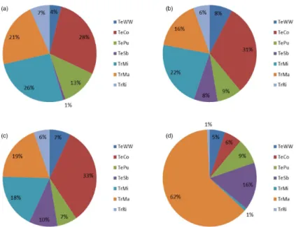
By performing the three optimizations for current climate we generated different sets
15
of optimal CFT distributions for each grid cell, optimization and time period. The op-timized fractions for current climate compared with the observed fractions taken from the SPAM dataset are shown in Fig. 1 as the mean over all grid cells. The distribu-tions from the two MPT optimizadistribu-tions were relatively similar to the observed ones, whereas for Opts,crop the distributions differed greatly, with TeCo and TrMa dominating
20
in the simulated case (Fig. 1). In the discussion below we mainly focus on the two MPT optimizations, as Opts,crop generally can be seen as a theoretical case, especially in
relation to subsistence farming.
The most striking difference between the observed fractions and the two MPT op-timizations was found for TeSb where the optimized fractions were∼10 times larger,
25
ESDD
5, 1571–1606, 2014Optimizing cropland cover for stable food
production in Sub-Saharan Africa
P. Bodin et al.
Title Page
Abstract Introduction
Conclusions References
Tables Figures
◭ ◮
◭ ◮
Back Close
Full Screen / Esc
Printer-friendly Version
Interactive Discussion
Discussion
P
a
per
|
Discussion
P
a
per
|
Discussion
P
a
per
|
Discussion
P
a
per
|
ca. 2 times larger, while the optimized TePu fractions were about two thirds to one half. The difference in crop distributions between the two individual MPT optimizations was relatively small, with 20 % larger fractions of TeSb and TrMa and 20 % lower fractions of TePu and TrMi for Opty,maxcompared to Optv,min(Fig. 1).
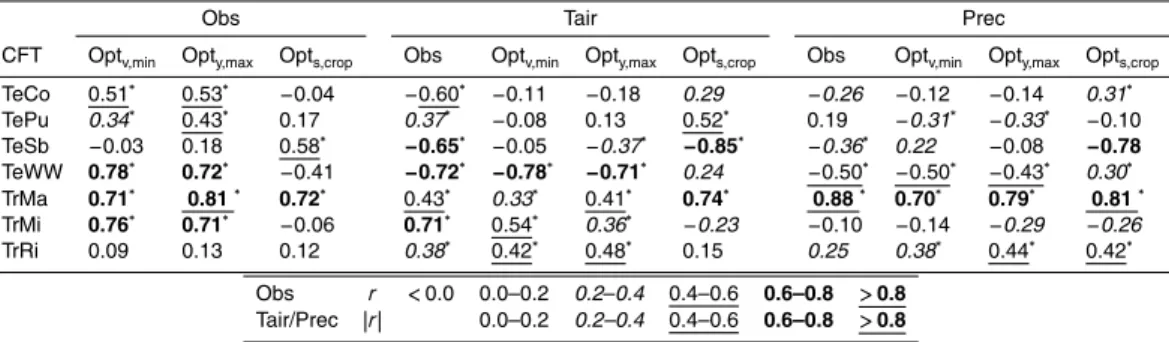
Latitudinally, the fractional cover of the three most important groups of crops in SSA
5
(based on number of calories produced, FAOSTAT, 2013) varied strongly for both opti-mized (Optv,minand Opty,max), and observed fractional crop cover (Fig. 2a–c). A strong positive correlation (p <0.001) was found between the optimized and observed frac-tions for all these CFTs (Table 2). For the remaining four CFTs the correlation was significant (for both Optv,min and Opty,max) for TeWW and TePu but not for TrRi and
10
TeSb. The largest differences between the mean observed and optimized fractions for TeSb, TrRi and TeWW were found between 10 and 25◦S (Fig. S1 in the Supplement). TeSb was the only CFT for which there was a significant correlation for Opts,crop and
not the MPT optimizations.
When performing the optimizations for future climate, the optimized fractional cover
15
changed slightly compared to the optimizations made for current climate. For both MPT optimizations there were relatively large increases over time in the areas of TrRi (Fig. S2). For Optv,minthere was a large increase in TrMi and a large decrease in TrMa
over time whereas for Opty,max there was relatively large increase for TePu. These
changes in CFT over time varied slightly with latitude (Figs. S3–S4). For Opts,crop
20
the dominating crops were TrMa and TeSb with a small relative increase in TrMa and a small decrease in TeSb for future climate (Figs. 1 and S2).
3.2 Spatial and temporal differences in yield and variance for Sub-Saharan Africa
In the optimization analysis the baseline values of Ypf and σ2 (Ypf, base and σbase2 )
25
ESDD
5, 1571–1606, 2014Optimizing cropland cover for stable food
production in Sub-Saharan Africa
P. Bodin et al.
Title Page
Abstract Introduction
Conclusions References
Tables Figures
◭ ◮
◭ ◮
Back Close
Full Screen / Esc
Printer-friendly Version
Interactive Discussion
Discussion
P
a
per
|
Discussion
P
a
per
|
Discussion
P
a
per
|
Discussion
P
a
per
|
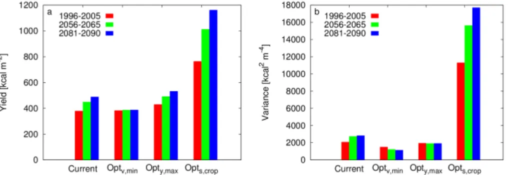
distribution from the observed ones. The optimized values of Ypf and σ2 were thus compared against the baseline values calculated based on the same (current or future) climate conditions but current observed crop distributions (Ypf, bclandσbcl2 ) meaning that Ypf, bcl=Ypf, baseandσbcl2 =σbase2 for current climate. The grid cell median value ofYpf, bcl for SSA was 380 kcal m−2with a median value forσbcl2 of 2100 kcal2m−4for current
cli-5
mate (Fig. 3). We chose median rather than mean, as for some grid cells the variance displayed extreme values (>1000 times larger than the median) which would have dis-torted the mean. Reflecting simulated yield increases in the future, a result mostly in response to enhanced atmospheric CO2 levels (Rosenzweig et al., 2013), there was
an increase inYpf, bclover time (Fig. 3a). For the majority of the grid cells (∼65 %), the
10
increase inYpf, bclwas also accompanied by an increase inσbcl2 leading to an increase in grid cell median σbcl2 over time (Fig. 3b). Following the definition of the two MPT optimization strategies, Optv,mingenerated a grid cell median value ofYpfand Opty,max
a median value ofσ2 close to their respective baseline values (Ypf, base andσbase2 ) for both future and current climate (Fig. 3). For Opts,cropbothYpfandσ
2
were much larger
15
thanYpf, bcl, andσbcl2 for current climate (100 and 440 % larger respectively), and both Ypfandσ2increased notably over time (Fig. 3a and b). The results from comparing the
difference between the optimized values ofYpfandσ2and the values ofYpf, bcl, andσbcl2 for current and future climates are presented below:
3.2.1 Minimizing variance while maintaining yield (Optv,min)
20
For current climate conditions, the set of assumptions that underlie optimization ap-proach Optv,min resulted in σ
2
ESDD
5, 1571–1606, 2014Optimizing cropland cover for stable food
production in Sub-Saharan Africa
P. Bodin et al.
Title Page
Abstract Introduction
Conclusions References
Tables Figures
◭ ◮
◭ ◮
Back Close
Full Screen / Esc
Printer-friendly Version
Interactive Discussion
Discussion
P
a
per
|
Discussion
P
a
per
|
Discussion
P
a
per
|
Discussion
P
a
per
|
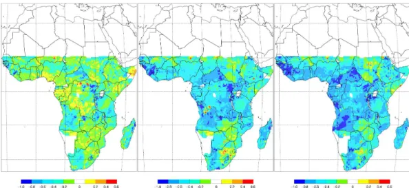
African Republic, Democratic Republic of Congo and Zambia) (Fig. 4a). For∼35 % of the grid cell this potential to decrease variance was>25 % (Table 3).
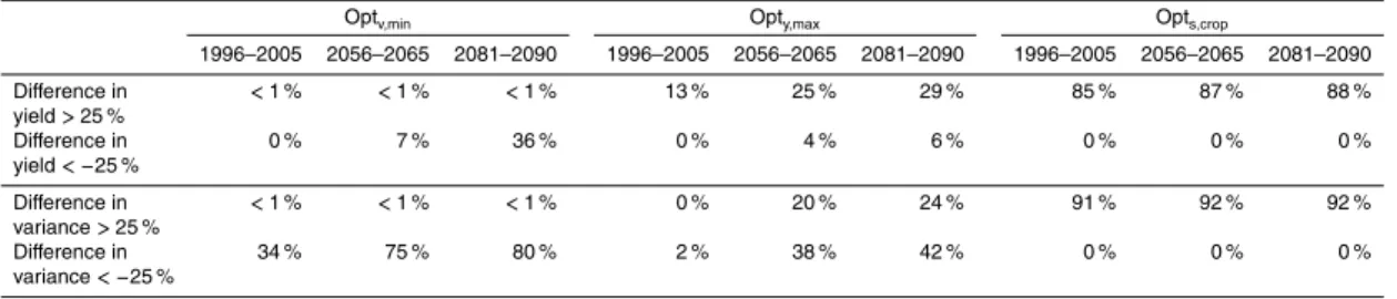
As a consequence of yield-increases over time being larger than the increase in variance (assuming current crop distribution), the potential of decreasingσ2 by crop selection became larger for future climate, mainly in central and western Africa (Fig. 4b
5
and c). For the two future time periods, a total of∼75–80 % of the grid cells displayed a potential to decreaseσ2by>25 % compared to assuming current crop distributions (σbcl2 ) (Table 3).
For current climate, there existed at least one set of crop fractions that fulfilled the first optimization criteria (Ypf> Ypf, base). For some grid cells (∼15 %) none of the crop
10
distributions that fulfilled the first optimization criterion displayed a lower variance than the baseline, meaning that optimization failed. These grid cells were mainly located in central and south western SSA. The number of grid cells for which the difference between optimized σbcl2 and variance assuming current crop distribution (σbcl2 ) was > 25 % was low (<1 %) (Table 3).
15
Whilst optimization of crop area following Optv,min was successful at reducing yield
variance, and this reduction was increased under future climate, this optimization fore-goes increases in yield that are projected to occur under current crop distribution (Fig. 3a). In other words, further reductions in variance are traded off against yield increases. This loss of future yield potential was largest in parts of the south
west-20
ern and of northeastern SSA (Fig. S5b and c). For the time period 2056–2065, yield for optimized crop distribution was>25 % lower compared to current crop distribution for∼10 % of the grid cells and for the time period 2081–2090 this figure was ∼35 % (Table 3).
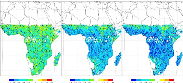
3.2.2 Maximizing yield while maintaining variance (Opty,max)
25
For current climate, the set of assumptions made in optimization approach Opty,max
ESDD
5, 1571–1606, 2014Optimizing cropland cover for stable food
production in Sub-Saharan Africa
P. Bodin et al.
Title Page
Abstract Introduction
Conclusions References
Tables Figures
◭ ◮
◭ ◮
Back Close
Full Screen / Esc
Printer-friendly Version
Interactive Discussion
Discussion
P
a
per
|
Discussion
P
a
per
|
Discussion
P
a
per
|
Discussion
P
a
per
|
was largest in southern SSA, and regionally in western and northeaster SSA (e.g. in the Democratic Republic of Congo and Kenya) (Fig. 5a). In total ∼15 % of the grid cells displayed the potential to increase yield by >25 % compared to using current crop distributions (Ypf, bcl) (Table 3).
Both the grid cell median optimized Ypf and Ypf, bcl increased slightly over time
5
(Fig. 3a). The difference between optimized Ypf and Ypf, bcl varied spatially and the largest potential to increase yield compared to assuming current crop distributions was found in western, southern and northeaster SSA as well as the Sahel (Fig. 5b and c).
Along similar lines as for Optv,min there existed at least one set of crop fractions
that fulfilled the first optimization criteria (σ2< σbcl2 ). For ∼10 % of the grid cells the
10
optimizedYpfhowever was lower thanYpf, bcl. For none of these grid cells the difference was>25 % (Table 3).
The optimizedσ2 for future climate were in many cases lower thanσbcl2 , largely be-cause the optimization for variance was made against σbase2 (current climate) and as grid cell medianσbase2 increased over time (Fig. 3b). For∼40 % of the grid cells, this
15
potential to decrease variance was>25 % (Table 3). In cases where σbcl2 decreased over time the difference instead became positive and for ∼20–25 % of the grid cells the relative difference between σ2 andσbase2 was>25 %. The largest potential of de-creasingσ2was found for central and western parts of SSA, while the largest increase in variance occurred in southern and northeaster SSA; as well as the Sahel (Fig. S6b
20
and c).
From the results above (Table 3) it can be seen that in case of Opty,max, it was
po-tentially possible to simultaneously increase yield and to decrease variance by 25 % for future climate compared to assuming current crop distribution for a number of grid cells. The number of grid cells for which both these criteria were met was∼5 %. By
25
contrast, if looking at the possibility to increase yield by 10 % instead, whilst decreasing variance by the same magnitude, the number of grid cells for which this occurred was
ESDD
5, 1571–1606, 2014Optimizing cropland cover for stable food
production in Sub-Saharan Africa
P. Bodin et al.
Title Page
Abstract Introduction
Conclusions References
Tables Figures
◭ ◮
◭ ◮
Back Close
Full Screen / Esc
Printer-friendly Version
Interactive Discussion
Discussion
P
a
per
|
Discussion
P
a
per
|
Discussion
P
a
per
|
Discussion
P
a
per
|
same time decreasing the yield variance are mainly located in western SSA, Angola and Tanzania (Fig. S7).
4 Discussion
The observed mean distributions of crops in SSA seem to follow the crop distributions from the two MPT optimizations for most crops relatively well (Figs. 1–2, Figs. S1–S2)
5
suggesting that farmers or farming systems in SSA indeed are following some risk aversion/yield maximization strategy. The significant correlation between the current latitudinal distribution of all crops (except TeSb and TrRi) and the MPT optimized distri-bution further supports this. In addition the relatively large number of optimization fail-ures (15 % for Optv,min and 10 % for Opty,max), indicates that current crop distributions
10
are relatively close to the optimum ones regionally (yellow to red colours in Figs. 4a and 5a).
The agreement is best for the dominating crops in SSA whereas the poorer agree-ment was found for the less important crops such as TrRi, TePu and TeSb. This sug-gests that MPT is a good method for interpreting the present-day general crop patterns
15
of major crops across SSA. The study was done for SSA, a region where subsis-tence farming is dominating. For agricultural regions in other continents or agricultural regions outside SSA additional drivers likely affect crop selection to a much larger de-gree. Examples of such drivers could be the maximization of profit (rather than the number of calories), or regional to local policies (e.g. EU subsidies). Therefore, the
20
difference found between optimized and observed crop fractional distribution for the southern parts of SSA might be explained by the dominance of commercial agriculture in these regions with the goal to rather maximize profit than the number of calories. In South Africa, which covers most of the land area south of 25◦S, commercial agriculture covers 86 % of total cropland (Anon., 2012). With wheat being a major cash crop, the
25
ESDD
5, 1571–1606, 2014Optimizing cropland cover for stable food
production in Sub-Saharan Africa
P. Bodin et al.
Title Page
Abstract Introduction
Conclusions References
Tables Figures
◭ ◮
◭ ◮
Back Close
Full Screen / Esc
Printer-friendly Version
Interactive Discussion
Discussion
P
a
per
|
Discussion
P
a
per
|
Discussion
P
a
per
|
Discussion
P
a
per
|
surprising, and the underlying assumptions of the MPT (based on optimizing the total amount of calories) may not work for these regions
Along similar lines, the optimization was made under the assumption that all crops where rained, whereas in reality in some regions a substantial percentage is irrigated (e.g. Balasubramanian et al., 2007) which can explain part of disagreement between
5
present-day optimized and observed crop fractions. In particular, the underestimation in optimized fractions of rice for the region between 17 and 25◦S could be explained by the large area of irrigated rice that can be found in Madagascar (Balasubramanian et al., 2007). Furthermore, the CFTs in LPJ-GUESS are not affected by pests, such that yields respond to climatic, but not biotic stresses. This might play a role particularly
10
for potatoes (TeSb) for which a large amount of pesticides is required compared to other crops in order to protect against, for example, late blight, a fungus responsible for large yield losses in unsprayed fields (Sengooba and Hakiza, 1999) with reported yield losses in central Africa of more than 50 % (Oerke, 2006).
Regardless of processes such as irrigation or pests, both temperature and
precipi-15
tation vary notably with latitude (Fig. 2d) such that the large latitudinal difference in the observed fractions of the different crops, including the most important ones for Africa (Fig. 2a–c), could be explained well by climate variability (Table 2). The latitudinal mean fractions of the different CFTs for the two MPT optimizations could in most cases be explained by the same climate variables (Table 2). The exceptions were TeCo and TeSb
20
where neither of the MPT optimized latitudinal distribution showed any correlation with temperature (TeCo) or precipitation (TeSb). For Optv,min there was also no correlation
between the optimized fractions of TeSb and temperature.
The strong correlation between observed fractions of both TrMi (positive) and TeWW (negative); and temperature and between TrMa and precipitation could be explained
25
ESDD
5, 1571–1606, 2014Optimizing cropland cover for stable food
production in Sub-Saharan Africa
P. Bodin et al.
Title Page
Abstract Introduction
Conclusions References
Tables Figures
◭ ◮
◭ ◮
Back Close
Full Screen / Esc
Printer-friendly Version
Interactive Discussion
Discussion
P
a
per
|
Discussion
P
a
per
|
Discussion
P
a
per
|
Discussion
P
a
per
|
is dominated by the northernmost and southernmost latitudes of SSA where tempera-tures are near the high (north) and low (south) end of optimum climate for maize (18– 33◦C) (Ecocrop, 2014). The large difference between optimized and observed fractions of TeWW, TeSb and TePu between 10 and 25◦S in our study indicate that the global model parameterization for these crops might not be ideal for the climatic conditions in
5
these regions.
Given the high correlation between observed and optimized crop distributions for cur-rent climate the distributions for future climate could be seen as scenarios of changes in crop distributions in regions where agriculture is focused on local sustenance. These types of scenarios could be alternatives to assuming no change in land use and crop
10
distribution as is frequently done in impact studies that focus on changes in yields (Rosenzweig et al., 2014; Schlenker and Lobell, 2010; Liu et al., 2008; Müller et al., 2010). Earlier studies looking at trends in crop selection have mostly done so from the perspective of societal demand for various crops (Wu et al., 2007). Our study in-stead focus on the supply side but taking into account also aspects of food production
15
stability, thus offering a complement to these types of studies.
For Opts,crop we identified the single highest yielding crop for current future climate. As simulated yield was normalized against observed yield this selection mainly repre-sents differences in yield from the SPAM dataset (You et al., 2013). The study by Franck et al. (2011) instead found the highest simulated yield (using LPJmL) for TeSb (in their
20
study named sugar beet) followed by TeCo (maize). The reason for these differences is likely mainly caused by the fact that they assumed intensive agricultural practices for all crops in order to compute maximum (potential) yield and did not normalize against observed (actual) yield.
In our study we investigated the ability to increase yield for a portfolio of crops while
25
ESDD
5, 1571–1606, 2014Optimizing cropland cover for stable food
production in Sub-Saharan Africa
P. Bodin et al.
Title Page
Abstract Introduction
Conclusions References
Tables Figures
◭ ◮
◭ ◮
Back Close
Full Screen / Esc
Printer-friendly Version
Interactive Discussion
Discussion
P
a
per
|
Discussion
P
a
per
|
Discussion
P
a
per
|
Discussion
P
a
per
|
through the selection of different rice varieties while keeping yield constant (Optv,min), or to increase profit by up to 23 % while keeping variance in yield constant (Opty,max)
(Nalley et al., 2009). Using the same approach, it was also possible to decrease cal-culated variance in wheat yield in north western Mexico by up to 33 % (Nalley and Barkley, 2010). The median ability to reduce variance or to increase yield in our study
5
was of the same order of magnitude, but with large spatial variability (Figs. 4–5). Other studies have found a large potential to increase food production by selecting the single highest yielding crop (Opts,crop) (Koh et al., 2013; Franck et al., 2011). In the
study by Koh et al. (2013) the highest yielding cereal (in t ha−1) (choosing between bar-ley, maize, millet, rice, sorghum and wheat) for each 5 min grid cell was selected using
10
data from Monfreda et al. (2008). Their results gave an increase in yield by 68 % in eastern Africa and 87 % in central Africa when selecting the highest yielding crop com-pared to current crop distribution. These results are lower than the increase in yield found from selecting the highest yielding crop in our study (Opts,crop). Their study
how-ever was confined to cereals and did not take into account any difference in dry weight
15
and calorie content of the different crops. As can be seen from our results, selecting the highest yielding crop generates not only a large increase in yield compared to cur-rent crop distribution but also an even larger increase in yield variance. Therefore this option is not a realistic one in most cases and should be seen as a theoretical rather than practical option.
20
Model impact studies have traditionally focused on changes in mean yield, ignoring the effect on variance. Some earlier studies exist on changes in future variance in yield (Urban et al., 2012; Chavas et al., 2009), but these studies looked at the effect of climate change on yield variability of single crops and not as was done in our study of a portfolio of crops.
25
ESDD
5, 1571–1606, 2014Optimizing cropland cover for stable food
production in Sub-Saharan Africa
P. Bodin et al.
Title Page
Abstract Introduction
Conclusions References
Tables Figures
◭ ◮
◭ ◮
Back Close
Full Screen / Esc
Printer-friendly Version
Interactive Discussion
Discussion
P
a
per
|
Discussion
P
a
per
|
Discussion
P
a
per
|
Discussion
P
a
per
|
obstacles for increasing yields due to, for example, high costs of fertilizers and lack of surface water for irrigation. Reducing the yield gap in SSA to a difference of 75 % be-tween actual and potential yield in general requires both increasing nutrient application and irrigated areas (Mueller et al., 2012). Switching from one mix of crops to another, maximizing yield while keeping an acceptable level of variance, as suggested by this
5
study might prove to be a cost-effective and food secure measure to produce more calories.
AgroDGVM models, like the LPJ-GUESS model used in this study, have the advan-tage of being able to simulate changes in yield and variance over large regions and for long time periods. This advantage comes at the price of lack in spatial detail and
sev-10
eral generalizations have to be made (related to e.g. soil types, local climate and crop management, and the effect of heat stress) (Rosenzweig et al., 2014; Bondeau et al., 2007). In addition, there are uncertainties related to model input. There may be biases in the climate input data generating possible errors, particularly in the variance of simu-lated yield. Our analysis was made using bias corrected climate data from 5 GCMs and
15
the median results from these model runs were used. Simulated fluxes of carbon using LPJ-GUESS have been shown to be highly sensitive to the choice of GCM (Ahlström et al., 2012). Averaging over several GCMs smooths some of the spatial and temporal variability from the individual GCMs, which will affect the calculated variance. To get realistic values of simulated yield these were normalized against yield from the SPAM
20
database. Variance in yield was however not normalized against measured data as the availability of realistic data for evaluating interannual variability in yield is limited. One potentially useful dataset is the one created by Iizumi et al. (2014) where reported data of harvested area for the year 2000, country yield statistics and satellite-derived net primary production were combined to generate a spatiotemporal gridded dataset
25
ESDD
5, 1571–1606, 2014Optimizing cropland cover for stable food
production in Sub-Saharan Africa
P. Bodin et al.
Title Page
Abstract Introduction
Conclusions References
Tables Figures
◭ ◮
◭ ◮
Back Close
Full Screen / Esc
Printer-friendly Version
Interactive Discussion
Discussion
P
a
per
|
Discussion
P
a
per
|
Discussion
P
a
per
|
Discussion
P
a
per
|
differences in the reporting of national yields. Secondly, the climate input data used in this study was based on GCM model runs which albeit having been bias corrected can-not be said to represent the actual climate variability for each individual grid cell even for current climate. Earlier validation tests for Africa have however shown the ability of LPJ-GUESS to reproduce interannual variability in maize yield at the country level as
5
reported by the FAO (Lindeskog et al., 2013).
This study investigated one aspect of food security, that is, the generation of a large and/or stable number of calories from existing cropland. From a food security per-spective many other factors are equally important, such as access to markets and the nutritional quality and safety of food. For example, not getting enough calories is only
10
one part of food safety problem. In addition to not getting enough calories, micronu-trient deficiency is a large problem with an estimated 2 billion people being affected (Tulchinsky, 2010). Also, at the same time as many people still suffer from malnutri-tion, obesity is a growing problem in the developing world (Godfray and Garnett, 2014; Steyn and Mchiza, 2014) meaning that people simultaneously can be both
undernour-15
ished and obese. This study focused on staple crops but for a fully nutritional diet these foods need to be complemented by foods which may be richer in minerals, vitamins and proteins (DeClerck et al., 2011).
5 Conclusions
The results from this study are based on the optimization of yield and variance for
20
groups of crops in SSA keeping yield or variance constant based on observed values for the current situation. This represents the trade-offbetween high yield and stable food production. The results show a potential to increase current or future yield and/or yield stability of a portfolio of crops by applying Modern Portfolio Theory to simulated crop yield.
25
ESDD
5, 1571–1606, 2014Optimizing cropland cover for stable food
production in Sub-Saharan Africa
P. Bodin et al.
Title Page
Abstract Introduction
Conclusions References
Tables Figures
◭ ◮
◭ ◮
Back Close
Full Screen / Esc
Printer-friendly Version
Interactive Discussion
Discussion
P
a
per
|
Discussion
P
a
per
|
Discussion
P
a
per
|
Discussion
P
a
per
|
follow the optimization rules of Modern Portfolio Theory for crop selection. Because of these similarities we suggest that our approach can be used to generate future sce-narios of sown areas for crops in SSA and likely similar regions, where food security is highly dependent on local food production. We also clearly demonstrate that selecting the highest yielding crop is not a valid option in regions such as SSA, as doing this
5
would generate unacceptably high variance in food production.
Our study highlights the great potential of Modern Portfolio Theory for answering questions about crop selection under current and future climate and its effect on yield and yield variability. It is possible to add further constraints to the optimization, for example by excluding crop distributions from the analysis that generate complete (or
10
near complete) crop failures for any one year. Depending on the scale of the study other aspects related to agriculture could be taken into account in the optimization, for example carbon storage in the soil, pesticide/fertilizer use and the nutritional value of various crops.
The Supplement related to this article is available online at
15
doi:10.5194/esdd-5-1571-2014-supplement.
Acknowledgements. This work was supported by the ClimAfrica project funded by the Eu-ropean Commission under the 7th Framework Program (FP7), grant number 244240 (http: //www.climafrica.net/). A. Arneth and T. A. M. Pugh also acknowledge support from the 7th Framework Program LUC4C (grant no. 603542). S. Olin was funded by the FORMAS Strong
20
ESDD
5, 1571–1606, 2014Optimizing cropland cover for stable food
production in Sub-Saharan Africa
P. Bodin et al.
Title Page
Abstract Introduction
Conclusions References
Tables Figures
◭ ◮
◭ ◮
Back Close
Full Screen / Esc
Printer-friendly Version
Interactive Discussion
Discussion
P
a
per
|
Discussion
P
a
per
|
Discussion
P
a
per
|
Discussion
P
a
per
|
References
Ahlström, A., Schurgers, G., Arneth, A., and Smith, B.: Robustness and uncertainty in terrestrial ecosystem carbon response to CMIP5 climate change projections, Environ. Res. Lett., 7, 044008, doi:10.1088/1748-9326/7/4/044008, 2012.
Anon.: Abstract of Agricultural Statistics, Department of Agriculture, Forestry and Fisheries,
5
Pretoria, South Africa, 2012.
Balasubramanian, V., Sie, M., Hijmans, R., and Otsuka, K.: Increasing rice production in Sub-Saharan Africa: challenges and opportunities, Adv. Agron., 94, 55–133, 2007.
Barrios, S., Ouattara, B., and Strobl, E.: The impact of climatic change on agricultural produc-tion: is it different for Africa?, Food Policy, 33, 287–298, 2008.
10
Berg, A., Sultan, B., and Noblet-Ducoudré, N.: Including tropical croplands in a ter-restrial biosphere model: application to West Africa, Climatic Change, 104, 755–782, doi:10.1007/s10584-010-9874-x, 2011.
Bondeau, A., Smith, P. C., Zaehle, S., Schaphoff, S., Lucht, W., Cramer, W., Gerten, D., Loetze-Campen, H., Müller, C., and Reichstein, M.: Modelling the role of agriculture for the 20th
cen-15
tury global terrestrial carbon balance, Global Change Biol., 13, 679–706, 2007.
Chavas, D. R., Izaurralde, R. C., Thomson, A. M., and Gao, X.: Long-term climate change impacts on agricultural productivity in eastern China, Agr. Forest Meteorol., 149, 1118–1128, 2009.
DeClerck, F. A., Fanzo, J., Palm, C., and Remans, R.: Ecological approaches to human nutrition,
20
Food Nutr. Bull., 32, 41S–50S, 2011.
Deryng, D., Sacks, W. J., Barford, C. C., and Ramankutty, N.: Simulating the effects of climate and agricultural management practices on global crop yield, Global Biogeochem. Cy., 25, GB2006, doi:10.1029/2009gb003765, 2011.
Di Vittorio, A. V., Anderson, R. S., White, J. D., Miller, N. L., and Running, S. W.: Development
25
and optimization of an Agro-BGC ecosystem model for C4 perennial grasses, Ecol. Model., 221, 2038–2053, doi:10.1016/j.ecolmodel.2010.05.013, 2010.
ESDD
5, 1571–1606, 2014Optimizing cropland cover for stable food
production in Sub-Saharan Africa
P. Bodin et al.
Title Page
Abstract Introduction
Conclusions References
Tables Figures
◭ ◮
◭ ◮
Back Close
Full Screen / Esc
Printer-friendly Version
Interactive Discussion
Discussion
P
a
per
|
Discussion
P
a
per
|
Discussion
P
a
per
|
Discussion
P
a
per
|
Fischer, G., Nachtergaele, F., Prieler, S., Teixeira, E., Tóth, G., van Velthuizen, H., Verelst, L., and Wiberg, D.: Global Agro-Ecological Zones (GAEZ v3.0): model documentation, Interna-tional Institute for Applied Systems Analysis (IIASA), Laxenburg, Austria and the Food and Agriculture Organization of the United Nations (FAO), Rome, Italy, 2012.
Foley, J. A., Ramankutty, N., Brauman, K. A., Cassidy, E. S., Gerber, J. S., Johnston, M.,
5
Mueller, N. D., O’Connell, C., Ray, D. K., and West, P. C.: Solutions for a cultivated planet, Nature, 478, 337–342, 2011.
Food and Agricultural Organisation: Food Balance Sheets, A Handbook, Rome, 2001.
Food and Agricultural Organisation: The State of Food Insecurity in the World 2013: The Multi-ple Dimensions of Food Security, Rome, 2013.
10
Franck, S., von Bloh, W., Müller, C., Bondeau, A., and Sakschewski, B.: Harvesting the sun: new estimations of the maximum population of planet Earth, Ecol. Model., 222, 2019–2026, doi:10.1016/j.ecolmodel.2011.03.030, 2011.
Gervois, S., de Noblet-Ducoudré, N., Viovy, N., Ciais, P., Brisson, N., Seguin, B., and Perrier, A.: Including croplands in a global biosphere model: methodology and evaluation at specific
15
sites, Earth Interact., 8, 1–25, 2004.
Godfray, H. C. J. and Garnett, T.: Food security and sustainable intensification, Philos. T. Roy. Soc. B, 369, 1–10, doi:10.1098/rstb.2012.0273, 2014.
Hickler, T., Smith, B., Sykes, M. T., Davis, M. B., Sugita, S., and Walker, K.: Using a generalized vegetation model to simulate vegetation dynamics in northeastern USA, Ecology, 85, 519–
20
530, 2004.
Hickler, T., Smith, B., Prentice, I. C., Mjöfors, K., Miller, P., Arneth, A., and Sykes, M. T.: CO2 fertilization in temperate FACE experiments not representative of boreal and tropical forests, Global Change Biol., 14, 1531–1542, 2008.
Iizumi, T., Yokozawa, M., Sakurai, G., Travasso, M. I., Romanenkov, V., Oettli, P., Newby, T.,
25
Ishigooka, Y., and Furuya, J.: Historical changes in global yields: major cereal and legume crops from 1982 to 2006, Global Ecol. Biogeogr., 23, 346–357, 2014.
Jarvis, A., Ramirez-Villegas, J., Herrera Campo, B. V., and Navarro-Racines, C.: Is cassava the answer to African climate change adaptation?, Trop. Plant Biol., 5, 9–29, 2012.
Knox, J., Hess, T., Daccache, A., and Wheeler, T.: Climate change impacts on crop productivity
30
ESDD
5, 1571–1606, 2014Optimizing cropland cover for stable food
production in Sub-Saharan Africa
P. Bodin et al.
Title Page
Abstract Introduction
Conclusions References
Tables Figures
◭ ◮
◭ ◮
Back Close
Full Screen / Esc
Printer-friendly Version
Interactive Discussion
Discussion
P
a
per
|
Discussion
P
a
per
|
Discussion
P
a
per
|
Discussion
P
a
per
|
Koh, L. P., Koellner, T., and Ghazoul, J.: Transformative optimisation of agricultural land use to meet future food demands, PeerJ, 1, e188, 2013.
Licker, R., Johnston, M., Foley, J. A., Barford, C., Kucharik, C. J., Monfreda, C., and Ra-mankutty, N.: Mind the gap: how do climate and agricultural management explain the “yield gap” of croplands around the world?, Global Ecol. Biogeogr., 19, 769–782, 2010.
5
Lindeskog, M., Arneth, A., Bondeau, A., Waha, K., Seaquist, J., Olin, S., and Smith, B.: Impli-cations of accounting for land use in simulations of ecosystem carbon cycling in Africa, Earth Syst. Dynam., 4, 385–407, doi:10.5194/esd-4-385-2013, 2013.
Liu, J., Fritz, S., Van Wesenbeeck, C., Fuchs, M., You, L., Obersteiner, M., and Yang, H.: A spa-tially explicit assessment of current and future hotspots of hunger in Sub-Saharan Africa in
10
the context of global change, Global Planet. Change, 64, 222–235, 2008.
Lokupitiya, E., Denning, S., Paustian, K., Baker, I., Schaefer, K., Verma, S., Meyers, T., Bernac-chi, C. J., Suyker, A., and Fischer, M.: Incorporation of crop phenology in Simple Biosphere Model (SiBcrop) to improve land-atmosphere carbon exchanges from croplands, Biogeo-sciences, 6, 969–986, doi:10.5194/bg-6-969-2009, 2009.
15
Markowitz, H.: Portfolio Selection: Efficient Diversification of Investments, 16, Yale University Press, Yale, 1959.
Matthews, R. B., Rivington, M., Muhammed, S., Newton, A. C., and Hallett, P. D.: Adapting crops and cropping systems to future climates to ensure food security: the role of crop modelling, Global Food Secur., 2, 24–28, 2013.
20
Meinshausen, M., Smith, S. J., Calvin, K., Daniel, J. S., Kainuma, M., Lamarque, J., Mat-sumoto, K., Montzka, S., Raper, S., and Riahi, K.: The RCP greenhouse gas concentrations and their extensions from 1765 to 2300, Climatic Change, 109, 213–241, 2011.
Monfreda, C., Ramankutty, N., and Foley, J. A.: Farming the planet: 2. geographic distribution of crop areas, yields, physiological types, and net primary production in the year 2000, Global
25
Biogeochem. Cy., 22, GB1022, doi:10.1029/2007GB002947, 2008.
Morales, P., Sykes, M. T., Prentice, I. C., Smith, P., Smith, B., Bugmann, H., Zierl, B., Friedling-stein, P., Viovy, N., and Sabate, S.: Comparing and evaluating process-based ecosystem model predictions of carbon and water fluxes in major European forest biomes, Global Change Biol., 11, 2211–2233, 2005.
30
ESDD
5, 1571–1606, 2014Optimizing cropland cover for stable food
production in Sub-Saharan Africa
P. Bodin et al.
Title Page
Abstract Introduction
Conclusions References
Tables Figures
◭ ◮
◭ ◮
Back Close
Full Screen / Esc
Printer-friendly Version
Interactive Discussion
Discussion
P
a
per
|
Discussion
P
a
per
|
Discussion
P
a
per
|
Discussion
P
a
per
|
Müller, C.: Climate Change Impact on Sub-Saharan Africa: an Overview and Analysis of Sce-narios and Models, German Development Institute/Deutsches Institut für Entwicklungspolitik (DIE), Bonn, 2009.
Müller, C., Bondeau, A., Popp, A., Waha, K., and Fader, M.: Climate change impacts on agri-cultural yields, World Bank, Washington, D.C., 2010.
5
Nalley, L. L. and Barkley, A. P.: Using portfolio theory to enhance wheat yield stability in low-income nations: an application in the Yaqui Valley of Northwestern Mexico, J. Agr. Resour. Econ., 35, 334–347, 2010.
Nalley, L. L., Barkley, A., Watkins, B., and Hignight, J.: Enhancing farm profitability through portfolio analysis: the case of spatial rice variety selection, J. Agr. Appl. Econ., 41, 641–652,
10
2009.
Oerke, E.-C.: Crop losses to pests, J. Agr. Sci., 144, 31–43, 2006.
Rockström, J., Folke, C., Gordon, L., Hatibu, N., Jewitt, G., Penning de Vries, F., Rwe-humbiza, F., Sally, H., Savenije, H., and Schulze, R.: A watershed approach to upgrade rainfed agriculture in water scarce regions through water system innovations: an integrated
15
research initiative on water for food and rural livelihoods in balance with ecosystem functions, Phys. Chem. Earth, 29, 1109–1118, 2004.
Rosenzweig, C., Jones, J., Hatfield, J., Ruane, A., Boote, K., Thorburn, P., Antle, J., Nelson, G., Porter, C., Janssen, S., Asseng, S., Basso, B., Ewert, F., Wallach, D., Baigorrial, G., and Winter, J. M.: The agricultural model intercomparison and improvement project (AgMIP):
20
protocols and pilot studies, Agr. Forest Meteorol., 170, 166–182, 2013.
Rosenzweig, C., Elliott, J., Deryng, D., Ruane, A. C., Müller, C., Arneth, A., Boote, K. J., Fol-berth, C., Glotter, M., Khabarov, N., Neumann, K., Piontek, F., Pugh, T. A. M., Schmid, E., Stehfest, E., Yang, H., and Jones, J. W.: Assessing agricultural risks of climate change in the 21st century in a global gridded crop model intercomparison, P. Natl. Acad. Sci. USA, 111,
25
3268–3273, doi:10.1073/pnas.1222463110, 2014.
Schlenker, W. and Lobell, D. B.: Robust negative impacts of climate change on African agricul-ture, Environ. Res. Lett., 5, 014010, doi:10.1088/1748-9326/5/1/014010, 2010.
Sengooba, T. and Hakiza, J.: The current status of late blight caused byPhytophthora infes-tans in Africa, with emphasis on eastern and southern Africa, in: Proceedings of the Global
30