Ricardo Pinho1,2*, Elhanan Borenstein3
, Marcus W. Feldman1
1Department of Biology, Stanford University, Stanford, California, United States of America,2PhD Program in Computational Biology, Instituto Gulbenkian de Cieˆncia, Oeiras, Portugal,3Department of Genome Sciences, University of Washington, Seattle, Washington, United States of America
Abstract
In this paper we study a model of gene networks introduced by Andreas Wagner in the 1990s that has been used extensively to study the evolution of mutational robustness. We investigate a range of model features and parameters and evaluate the extent to which they influence the probability that a random gene network will produce a fixed point steady state expression pattern. There are many different types of models used in the literature, (discrete/continuous, sparse/dense, small/large network) and we attempt to put some order into this diversity, motivated by the fact that many properties are qualitatively the same in all the models. Our main result is that random networks in all models give rise to cyclic behavior more often than fixed points. And although periodic orbits seem to dominate network dynamics, they are usually considered unstable and not allowed to survive in previous evolutionary studies. Defining stability as the probability of fixed points, we show that the stability distribution of these networks is highly robust to changes in its parameters. We also find sparser networks to be more stable, which may help to explain why they seem to be favored by evolution. We have unified several disconnected previous studies of this class of models under the framework of stability, in a way that had not been systematically explored before.
Citation:Pinho R, Borenstein E, Feldman MW (2012) Most Networks in Wagner’s Model Are Cycling. PLoS ONE 7(4): e34285. doi:10.1371/journal.pone.0034285
Editor:Matjazˇ Perc, University of Maribor, Slovenia
ReceivedFebruary 10, 2012;AcceptedFebruary 25, 2012;PublishedApril 12, 2012
Copyright:ß2012 Pinho et al. This is an open-access article distributed under the terms of the Creative Commons Attribution License, which permits unrestricted use, distribution, and reproduction in any medium, provided the original author and source are credited.
Funding:The Ph.D. Program in Computational Biology is sponsored by Fundac¸a˜o Calouste Gulbenkian, Siemens SA, and Fundac¸a˜o para a Cieˆncia e Tecnologia (fellowship SFRH/BD/33531/2008). The research was also supported in part by National Institutes of Health grant GM28016 and National Science Foundation award CNS-0619926. The funders had no role in study design, data collection and analysis, decision to publish, or preparation of the manuscript.
Competing Interests:The Ph.D. Program in Computational Biology is sponsored by, among others, Siemens SA. There are no competing interests or relationship between the authors and this commercial funder, besides that. This does not alter the authors’ adherence to all the PLoS ONE policies on sharing data and materials.
* E-mail: [email protected]
Introduction
Gene regulatory networks have been studied intensively in recent years, both by physicists and biologists, who have provided different insights into this important field [1,2]. We present numerical simulations to investigate stability in large Random Threshold Networks (RTNs) [3]. This spin glass or neural network-type model [4] represents a subclass of Random Boolean Networks (RBNs) [5]. We consider all attractor types rather than only those networks that have fixed points. Thus our framework is that used by physicists [6,7] rather than that used by biologists [8,9].
Wagner [8,10] introduced a version of this gene network model to study the evolution of genetic robustness. The gene network is represented by a dynamical system whose state variables correspond to expression levels of the network’s genes. A network is said to be robust if it retains the same expression state after mutation. The transient from an initial state to an attractor represents a developmental process and the fixed point attractor represents the phenotype. For this reason, fixed points have been traditionally considered developmentally stable, and networks that have cycling dynamics are not allowed to survive. This requirement of developmental stability [9] can be viewed as viability selection [11]. Implementations of the model for evolutionary simulations have varied in parameters such as network size, connectivity, normal-ization function, and whether the components of both the state vector and the matrix are discrete or continuous [8,9,11–22]. In principle, all of these parameters may influence the dynamics of the model and, consequently, the results of evolutionary simulations. It is well known, for example, that prior to evolution, smaller networks are more robust to mutations than larger ones,
and that this relationship reverses after selection [8]. Our goal is to systematically explore how changes in all of these parameters affect the probability of fixed points, in the hope of motivating discussion of the relevance of this model for evolutionary analysis. To this end,we focus our attention solely on the gene network model itself, on what has been called developmental dynamics, without evolution. We generate millions of random networks of size up toN~10,000and measure the probability of fixed point dynamics for most of the different parameterizations reported in the literature, and show that cycles always dominate network dynamics. Fixed point steady states are the exception, not the rule in this gene network model. We also show that stability, defined as the probability of fixed point dynamics, decreases with network size and density. Stability distributions are bimodal: some matrices are always stable independently of the initial state, while others never reach a fixed point. Other measurements like period-size distributions show further deviation of the properties of this network model from those of the general class of RBNs.
The layout of the paper is the following: we finish the Introduction by presenting a more detailed version of the Model; we next present our Results (more of which are detailed in Text S2 and Supporting Information Figures), followed by a Discussion; we conclude with a short Methods section where we present a summary of each model variant used to produce our Figures (Table S1; more detailed methods can be found in Text S1).
Model
the effect on gene i of the product of gene j. The matrix is generally not symmetric and diagonal elements,wii, represent self-regulation. The fractioncof nonzero entries in theW matrix is a parameter of the model and reflects the density of the network. The degree of a gene is represented byKiandSKT~cN, 0ƒcƒ1 is called network connectivity [23,24]. Each network is a dynamical system, with state vectorS(t)~ðs1(t),:::,sN(t)Þ repre-senting the expression levels of each gene at time t. The deterministic, discrete-time dynamics ofS(t)are modeled by the set of nonlinear coupled difference equations
si(tz1)~f
XN
j~1 wijsj(t)
" #
, ð1Þ
wheref is a normalization function that prevents the system from diverging (Text S1). More specifically, f is a threshold function (either step or sigmoid; Figure S13), representing cooperative binding and saturation in gene expression. The network is updated synchronously (see [25–27] for asynchronous updates). We define Equation (1) as the development process (see [8,9] for an illustration of the model, as well as a discussion of the biological motivations and assumptions behind it). Since the state space of the model is finite and the dynamics deterministic, the system will eventually reach an attractor given an initial gene expression state. The attractor can either be a fixed point or a limit cycle.
The simplicity of the model allows for evolutionary simulations, where a standard population genetic model of mutation, recombination and selection acts upon a population of gene networks, and the network’s state is taken as its phenotype. Despite their level of abstraction, Boolean networks have been highly successful, both at reproducing experimental results in different
organisms [2,18,28,29], and allowing for theoretical predictions about the evolution of network properties such as robustness, evolvability, and many others [8,9,11,13–17,19–22,30–38].
The properties of this gene network model in the absence of evolution or any kind of selection have attracted considerably less attention in the genetic regulation literature [11,12,18,20,30,31]. On the other hand, the physics community has been studying some theoretical properties of RBNs for some time (see [6,7] for recent reviews). In RBNS, each node is assigned an update function that prescribes the state of the node in the next time step, given the state of its input nodes. This update function is chosen from the set of all possible update functions according to some probability distribution. Since each of theKinputs of a node can be on or off, there areM~2K possible input states. The update function has to specify the new state of a node for each of these input states. Consequently, there are2Mdifferent update functions [7]. RTNs are boolean networks with threshold functions only. The update function is Equation (1) withf(x)~sgn(x)(Text S1). While some analytical results have been obtained for the general class of RBNs, they usually apply only under some restricted conditions, such as in the limit of very large networks, specific network connectivities, or combinations of boolean functions. It has been shown that some results derived under these assumptions break down when only a subset of boolean functions is considered [39–41]. This is the case for RTNs, and although interesting in their own right, theoretical work done with RTNs seems to have been limited [3,24,42,43].
Results
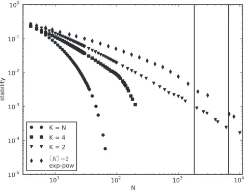
As we can see in Figure 1, cycles seem to dominate the dynamics, independently of network size N and degree K.
Figure 1. Cycles dominate the dynamics.Average stability (Equation (2)) for different network sizesN, degreeKand topology.K~Nmeans c~1. Equation (1) is solved up ton~108times withw
ij*N(0,1),si*f{1,1g,f(x)~sgn(x)andsgn(0)~1. Noisy tails forK~2result from insufficient
samples (Figure S4). Our measure is binary (the outcome is either0or1for each trial) and, for that reason, we do not find it helpful to present a variance measure. Instead, we present full stability distributions for similar experiments in Figure 2. Boxed region represents the size of the genome-wide regulatory networks ofE. coli[45] and yeast [47].
Stability (Equation (2) in Methods) has a maximum of 0:26 for N~4,K~2, and decreases monotonically in both parameters. ForK~2, stability decreases almost as a power-law inN, and this decrease is faster for larger K. A minimal stability value of
2:5|10{6is found forN~K~60. Small networks ofN~K~4 genes are about3times more likely to reach a cycle than a fixed point steady state. For N~K~10, cycles are *12 times more likely.
Also represented is a non-regular biological topology, with exponential in-degree distribution, and scale-free out-degrees (Text S1, Text S2, Figure S1 and Figure S2; see Table S2 and Figure S3 for transient times and Figure S4 for sample sizes).
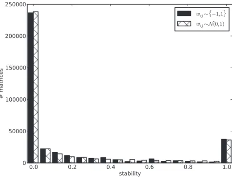
Figure 1 depicts the average stability for networks of different sizes. We next ask if this average is a good proxy for typical network behavior. In other words, what is the stability distribution for networks of a given size? Figure 2 shows that this distribution is bimodal, where some matrices are never stable, independently of the initial state, while others always reach a fixed point from every initial state. This suggests there could be two type of matrices in this model: unstable and stable ones, with the former being much more common than the latter. Interestingly, if we increase network size toN~10 and sample random binary matrices, we still find both types of matrices, but with a more uneven distribution. We find 1928 matrices with stability~0 in our random sample of N~10, against87withstability~1: a22-fold difference.
We next ask how network density,c, affects stability. As we can see in Figure 3, stability goes down with increasingc, and has a maximum value of0:23 for N~5and minimalc. Again, cycles dominate the dynamics, independent of network density, but sparser networks seem more stable. Although sparse networks of sizeN~10with one or two regulatory inputs per gene (c~0:1and
0:2) only have stability*0:14, they are almost twice as stable as dense networks withc~1.
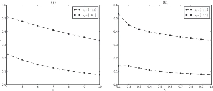
So far we have represented the off state of a gene by{1, and although this seems to be the most common choice in the literature, some authors use0to represent the off state [18,19]. As shown in Figure 4, stability is higher in thef0,1gthan thef{1,1g map, and it goes down linearly with bothN andc. The slope of this decay is about the same for both maps, resulting in a2*4fold difference in stability between the two. Interestingly, the f0,1g map produces the only instances for which reaching a fixed point is actually more likely than a cycle. This is the case forN~4,c~1
and N~10, c~0:1. In fact, using the f0,1g map, stability is always greater than0:5for the sparsest(K~1)network of any size (Figure S6; see Text S2, Figure S7 and Figure S8 for more comparative studies of the two representations).
In Figure 5 we show that stability distributions are very similar for binary and real matrices, with the real set having slightly more unstable and fewer stable matrices than the binary one. To see whether the same is true of the normalized means of the distributions, i.e., the networks’ average stability, we return to Figure 1 and see that forN~4we find a stability value around
0:23, estimated by randomly sampling106real matrices. Random sampling of106binary matrices estimates stability around0:31. A full enumeration of the total65,536binary matrices (N~4) yields *0:37 stability. It seems that random sampling over-represents unstable matrices, which are the most frequent ones in the full distribution.
Finally, we compare stability for binary and real states. Figure 6 shows that the stability distributions are similar with either the sign (binary) or the steep sigmoid (real) functions witha~10,100and evena~2for allNandcw0:1. This is somewhat expected if you
Figure 2. Stability distribution is bimodal.Two types of matrices: stable (stability~1) and unstable (stability~0). Full enumeration of binary network space forN~4 2N2
~65,536
and a random sample of3876binary matrices forN~10. Full enumeration of the state space for both cases
2N
ð Þ. ForN~4, each bin corresponds to a specific stability value. There are a total of26,135unstable (first bin) and16,574stable (last bin) matrices in the genotype space of binary matrices of sizeN~4. ForN~10, different stability values are binned together in17bins of width*0:06each. For that
reason, not allN~10matrices included in the first bin havestability~0, for example. There are1928unstable matrices versus87stable ones in our random sample ofN~10.c~1; other parameters are as in Figure 1.
compare these different normalization functions in Figure S13. In fact, lim
a?? z(x;a)~sgn(x). We also note that stability starts to behave differently for lowa~1(Text S1, Text S2 and Figure S9).
More results are presented in Text S2.
Discussion
In this study, we have conducted extensive simulation analysis of a subclass of random Boolean networks, known as Random
Threshold Networks (RTNs). We defined stability as the probability of reaching a steady state and investigated the dependence of stability on network size and density, types of regulatory interactions and gene expressions and parameter values. The main findings are:
1. There are vastly more cyclic solutions than steady state solutions; only the latter have been assumed to be ‘‘viable’’ networks in previous studies.
Figure 3. Sparser networks are more stable.Average stability (Equation (2)) for different network densitiesc~fK=N: K~1,2,:::,Ngand sizes
N~5,10,20. Equation (1) is solved up ton~108times for eachcandN. Other parameters as in Figure 1. Dashed lines are guides to the eye. Shaded
region represents the density of biological networks [32,45]. doi:10.1371/journal.pone.0034285.g003
Figure 4. Stability is2*4fold higher with thef0,1g(squares) than thef{1,1g(circles) maps.Equation (1) is solvedn~106times for each N,c~1(a) andc,N~10(b) withwij*N(0,1). For thef{1,1gmap:si*f{1,1g,f(x)~sgn(x),sgn(0)~1. For thef0,1gmapsi*f0,1g,f(x)~H(x),
2. Some networks never cycle while others always cycle independently of the initial conditions.
3. Sparse networks are stable more often than dense networks. 4. Using0instead of{1to represent the off state induces more
stable solutions. However, for well connected networks, stable states are discovered more rapidly for{1networks.
5. Binary and real valued weight matrices have similar stability properties.
6. Discrete or continuous gene expression states may give similar results, depending on the steepness of the sigmoid function. 7. Network topology seems to have a small effect on stability 8. The distribution of attractor lengths appears to decay more
slowly than the typical power law.
All of these results may have implications for both the use of the RTN as a model of gene regulation and the properties of real biological networks. For brevity, we focus solely on the former. Figure 5. Binary and real matrices seem to have the same stability distribution.Equation (1) is solved for2sets of376,992random matrices each, and full enumeration of state space ð2N~32Þ. N~5, c~1, s
i*f{1,1g, f(x)~sgn(x), sgn(0)~1. wij*f{1,1g for binary matrices and
wij*N(0,1)for real ones.
doi:10.1371/journal.pone.0034285.g005
Figure 6. Steep sigmoid functions result in the same stability profiles as the sign function.Average stability (2) for different network sizes N,c~1(a) and densitiesc,N~10(b) with different normalization functionsf(x). Equation (1) is solvedn~106times withw
ij*N(0,1),si[½{1,1, f(x)~sgn(x)withsgn(0)~1for the first curve, and the sigmoidf(x)~z(x;a)for all curves identified by steepnessa(Text S1). Forz(x;a), other
This is the first time networks of the size of an organism have been simulated with this model. To the best of our knowledge, the largest network previously studied has N~400 genes [44]. We have extended this range to N~10,000 (Figure 1). This is comparable to E. coli (*1,800 genes identified in its regulatory network [45] or*4,300annotated genes in the genome of the K-12 strain [46]) and to yeast (3,420network genes [47] or*5,8000 annotated genes in the Saccharomyces cerevisiae genome [48]). We have also seen that stability seems to decay much faster for degree K~N than for smaller K. For networks of size N~65, for example, the probability of fixed points is already smaller than
10{4. More importantly, this number seems to approach 0for largerN, unlike the fat tails ofK~2. In other words, by choosing K~N, one cannot study stable states for organism-size, genome-wide networks. Interestingly, dense networks are the most popular choice in the literature [16,22]. Our results have clear implications for the interpretation of previous studies [8,16]. By limiting their analysis to small dense networks with stable dynamics, most previous findings are limited in reach and may not apply to real biological networks.
Figure 2 clearly suggests there are two types of networks in this model: stable and unstable. This bimodal nature of the stability distribution is not trivial. It is interesting that the stability of a random pair of matrix and initial state tells us how likely it is that the matrix is stable (or not) with any other random initial state. It is the network that determines stability, not the initial state. This implies that future studies using this model do not have to sample many different initial states to characterize network dynamics. Sampling pairs of networks and initial states, as we have done in most of our study, should suffice. These two classes of networks may have different topological properties. Since previous studies only use viable networks, most of the networks they allow to evolve are of the second type, i.e., stable. It is true that we do not expect biological networks to be random; the question is if we do want to start our simulations from a non-random set, are the chosen matrices biologically relevant? And, by selecting these and not others, what properties or biases are introduced into the simulations, prior to evolution? To the best of our knowledge, these questions have yet to be addressed.
A great deal has been written about scale-free networks in biology [49,50]. In contrast, most networks we have studied here are regular, since this is the topology frequently used with gene regulatory networks [8,9], and thus the ones we are interested in characterizing. We have shown, however, that different topologies, including scale-free out-degree distributions, do not seem to change the overall results, in agreement with previous studies [22,34].
In Figure 3 we see that stability seems to decay faster withcfor larger networks and in Figure S5 we have tried to show this explicitly finding that for small to intermediate size networks (N~10*20), the difference between the stability of dense and sparse networks is maximized. This is about the size of networks used in previous studies [11,33], where networks with different densities coexist in a population (i.e. adding or deleting connections is allowed). We believe this stability difference should be taken into account in analysis of such studies. Further, network stability does not seem to depend strongly on the nature of the matrix weights, either binary or real-valued (Figure 5).
An important parameter of the model is how cells respond to their input signals. That is to say, is gene regulation a switch-like process, or is the response graded? While the former is implemented by a step function, the latter is modeled as a sigmoid curve (Figure S13). One could argue that a switch-like mechanism already introduces a lot of robustness to the model, in the sense that most changes do not produce a visible change in the
phenotype (for xw0 or xv0 in the figure). Sensitivity sharply increases, however, at DxD?0, where the discontinuity occurs. Close to zero, very small changes in the regulatory inputs of a gene can quickly turn it on or off. In thisDxD?0region, the system is clearly not robust. The opposite can be said of a not very steep sigmoid function. By allowing continuous expression values, small changes inxlead to small changes in a gene’s states~f(x). This choice, however, allows changes in positive or negative inputs aroundDxDw1(or evenDxDw5) to still produce visible changes in phenotype. In this sense, the system is less robust. We have shown that the two choices are only equivalent, at least in terms of stability, for large a, where the sigmoid behaves almost like a switch (Figure 6). With smalla, for which the sigmoid is less steep and behaves more like a gradient, the choice between a step [8,14] or a sigmoid function [9,16] makes a difference (see Text S2 and Figure S12 on how to deal withf(0)in the discrete case).
As already mentioned, a lot of work has been done on analytical properties of Random Boolean Networks [23,51] and it has been suggested that some properties of RTNs do not follow analytical results derived for the general class of RBNs [39–41]. The dynamics of RBNs with canalizing functions only, for example, seem to be dominated by fixed points [52]. We have shown here that this is clearly not the case for RTNs. It has also been suggested that the attractor length distribution of RBNs follows a power-law [7,40]. Again we have shown this is not true for RTNs, which instead seem to follow an exponential decay for a range of parameters (Figure S10 and Figure S11) perhaps slightly slower than initially suggested [43].
Methods
The attractor reached by the dynamical system (1) is uniquely defined by the matrixWand the initial stateS(0), and is either a fixed point or a cycle. Letnrepresent the number of pairs ofW andS(0)for which Equation (1) is solved, andnfƒnthe number of times the attractor is a fixed point. To estimate the probability of reaching a fixed point steady state within the framework of this model, we generated up ton~108random pairs of matrices and initial states, for different network sizesN and degrees K, and measured
stability~nf=n, ð2Þ
which takes values between0and1. The estimated probability of cycles is given by1{stability.
As mentioned before, most of the evolutionary studies done with this model vary in the parameters used in Equation (1). We estimate the dependence of stability measured by Equation (2) on most of these parameters. We list in Table S1 all the variations we have studied along with the corresponding figures and references. Special relevance is given to the range of parameters used in previous studies. For this reason, we mostly study small [8,9] and dense [16,22] networks. Real gene networks, however, can be quite large [45,47] and appear to be sparsely connected, with an average of two transcriptional regulators per gene [32]. Stability estimates are also shown for these more realistic topologies [49,53].
More detailed methods and algorithms are included in Text S1.
Supporting Information
Text S1 Supporting Methods.More details on experimental procedures and algorithms for solving Equation (1) for both the discrete and continuous cases.
Text S2 Supporting Results. More results exploring the dependence of stability on parameters of the model. More parameters are also explored. Sample sizes and transient times are analyzed too.
(PDF)
Figure S1 Stability decreases withNeven for scale-free biological topologies.Average stability (Equation (2)) is plotted for different network sizes N and topology. SKT~2. Ki~2for every gene,i, in the regular network. The Poisson network draws the degree distributions from a Poisson distribution with mean and variance equal to 2. exp-pow stands for exponential in-degree distribution, and power-law out-degree distribution, both with mean2. Other parameters as in Figure 1.
(EPS)
Figure S2 Stability decreases withNin spite of topology forK~4.Same as Figure S1 forSKT~4. In this case we do not represent the biological topology, since biological networks usually haveSKT*2[32].
(EPS)
Figure S3 Path length to equilibrium grows rapidly with N.Represented is average transient time (i.e. the number of time steps until the network reaches an attractor) as a function of network sizeNand for different degreesK. Only fixed points are considered. Equation (1) is solved up to n~108 times with parameters as in Figure 1. Although coefficients of a least-squares fit are shown in the figure legend for eachK, these regression lines are presented here only as a qualitative description. The estimates are employed for the extrapolation of transient times of larger networks, used to impose a cut-off on the convergence time of Equation (1). Error bars are big but are not shown to avoid cluttering the figure.
(EPS)
Figure S4 Sample size decreases with increasing N. Shown is the number of samples from which the results presented in Figure 1 are drawn. Increase of convergence time withN, as depicted in Figure S3, limits sample size.
(EPS)
Figure S5 The effect of network degree on stability seems to depend on network size. Represented is
stabilityðK~K’Þ{stabilityðK~NÞ
½ for different K’~2,4,6
and N. It seems that the difference in stability between sparse networks and the densest one has a maximum for an intermediate Nw10. After an initial increase, it goes down with increasingN, wherestability(K~N)?0, and thus the difference is reduced to stability(K~K’). This basically represents the difference between the different plots in Figure 1.
(EPS)
Figure S6 Stability is higher than0:5for thef0,1gmap with K~1. The f0,1g map produces the only case where reaching a fixed point is actually more likely than reaching a cycle for any network size. This happens, however, for the uninteresting case of K~1 regular networks, where each gene receives input from only one other gene, or itself. Equation (1) is solved up to n~108 times for each N and K with w
ij*N(0,1), si*f0,1g, f(x)~H(x)andH(0)~1(Text S1).
(EPS)
Figure S7 The f0,1g map has more stable and less unstable matrices than f{1,1g. Equation (1) is solved for N~4,c~1, wij*f{1,1gand full enumeration of the network
2N2
~65,536
and stateð2N~16Þspaces. Other parameters are as in Figure 4.
(EPS)
Figure S8 Thef{1,1gmap and real matrices allow for faster discovery of novel phenotypes.Shown is the number of samples needed to reach all 1024 fixed point attractors of networks of sizeN~10, for different cand maps (a) or types of regulatory interactions (either binary or real) (b). Equation (1) is solved up ton~109 times for each c. For c~0:1 and 0:2, the f0,1gmap reaches the maximum sample size before the discovery of all stable phenotypes. The results shown are for one run only. Other parameters are as in Figure 4 (a) and Figure 5 (b). (EPS)
Figure S9 Stability is not monotonic in a. Although still low, the probability of fixed points has a maximum for
0:7vav0:8. Stability also seems slightly higher fora~100than a~10. Equation (1) is solved n~106 times with wij*N(0,1), N~10, c~1, si[½{1,1and sigmoidal f(x)~z(x;a), varying a (Text S1). Other sigmoid parameters are as in Figure 6. The dashed line is a guide to the eye.
(EPS)
Figure S10 Probability of attractor length decays slower than a power-law.Shown is the attractor period distribution for the two different maps and networks of size and density N~K~10. The f{1,1g map has an antisymmetric property where cycles of even length are overrepresented at least 2-fold (Figure S11; [12,31]). For that reason, even and odd periods are analyzed separately. Also shown is a least-squares fit for thef0,1g map. Equation (1) is solved with parameters as in Figure 4. (EPS)
Figure S11 Cycle size distribution for thef{1,1gmap. Represented is the attractor size distribution, as in Figure S10, but just for thef{1,1gmap with the odd and even length cycles taken together. Note how cycles of even length are overrepresented at least 2-fold.
(EPS)
Figure S12 Different conventions for f(0) result in similar stability profiles. Stability is shown for different N and definitions off(0)(Equation (1)). Networks are regular and binary, wij*f{1,1g. random means we choose f(0)~1 or {1 with equal probability. f(0)~S(t{1) means si(t)Df(0)~si(t{1). si*{1,0,1for the latter and also forf(0)~0.
(EPS)
Figure S13 The sign and sigmoid functions are very similar fora§10.The parameteracontrols the steepness of the sigmoid function,z(x;a), where lim
a??z(x;a)
~sgn(x)(Text S1). (EPS)
Table S1 List of all model variants and corresponding figures and references. Most of the evolutionary studies done with this model vary in the parameters used in Equation (1). We estimate the dependence of stability measured by Equation (2) on most of these parameters. (PDF)
Table S2 Limits on transient times as a function ofN andK. Table entries are the range ofNvalues for which eachT is used. The time it takes for Equation (1) to reach an attractor grows with N (Figure S3). To be able to produce Figure 1, a time limit T(N;K)v?is enforced for large or dense networks.
Acknowledgments
RP would like to thank Daniel Weissman, Amanda Casto and Robert Furrow for helpful discussions throughout the course of this work, Jeremy Van Cleve and Michael E. Palmer for technical support, and Isabel Gordo and Tiago Paixa˜o for helpful comments and insights. Special thanks to Manuel Irimia for all the guidance and help.
Author Contributions
Conceived and designed the experiments: RP EB MF. Performed the experiments: RP. Analyzed the data: RP. Wrote the paper: RP MF.
References
1. Bornholdt S (2005) Systems biology. Less is more in modeling large genetic networks. Science 310: 449–451.
2. Bornholdt S (2008) Boolean network models of cellular regulation: prospects and limitations. J R Soc Interface 5: S85–S94.
3. Ku¨rten KE (1988) Correspondence between neural threshold networks and Kauffman Boolean cellular automata. J Phys A: Math Gen 21: L615–L619. 4. Hopfield JJ (1982) Neural networks and physical systems with emergent
collective computational abilities. Proc Natl Acad Sci U S A 79: 2554–2558. 5. Kauffman SA (1969) Metabolic stability and epigenesis in randomly constructed
genetic nets. J Theor Biol 22: 437–467.
6. Aldana M, Coppersmith S, Kadanoff LP (2003) Boolean dynamics with random couplings. In: Kaplan E, Marsden JE, Sreenivasan KR, eds. Perspectives and Problems in Nonlinear Science. A Celebratory Volume in Honour of Lawerence Sirovid. Berlin: Springer. pp 23–89.
7. Drossel B (2008) Random Boolean Networks. arXiv:07063351v2 [cond-matstat-mech].
8. Wagner A (1996) Does evolutionary plasticity evolve? Evolution 50: 1008–1023. 9. Siegal ML, Bergman A (2002) Waddington’s canalization revisited: develop-mental stability and evolution. Proc Natl Acad Sci U S A 99: 10528–10532. 10. Wagner A (1994) Evolution of gene networks by gene duplications: a
mathematical model and its implications on genome organization. Proc Natl Acad Sci U S A 91: 4387–4391.
11. Ciliberti S, Martin OC, Wagner A (2007) Robustness can evolve gradually in complex regulatory gene networks with varying topology. PLoS Comput Biol 3(2): e15. doi:10.1371/journal.pcbi.0030015.
12. Huerta-Sanchez E, Durrett R (2007) Wagner’s canalization model. Theor Popul Biol 71: 121–130.
13. Draghi JA, Wagner GP (2009) The evolutionary dynamics of evolvability in a gene network model. J Evol Biol 22: 599–611.
14. Bornholdt S (2001) Modeling genetic networks and their evolution: a complex dynamical systems perspective. Biol Chem 382: 1289–1299.
15. Kaneko K (2007) Evolution of robustness to noise and mutation in gene expression dynamics. PLoS One 2: e434.
16. Azevedo RBR, Lohaus R, Srinivasan S, Dang KK, Burch CL (2006) Sexual reproduction selects for robustness and negative epistasis in artificial gene networks. Nature 440: 87–90.
17. Palmer ME, Feldman MW (2009) Dynamics of hybrid incompatibility in gene networks in a constant environment. Evolution 63: 418–431.
18. Li F, Long T, Lu Y, Ouyang Q, Tang C (2004) The yeast cell-cycle network is robustly designed. Proc Natl Acad Sci U S A 101: 4781–4786.
19. Masel J (2004) Genetic assimilation can occur in the absence of selection for the assimilating phenotype, suggesting a role for the canalization heuristic. J Evol Biol 17: 1106–1110.
20. McDonald D, Waterbury L, Knight R, Betterton MD (2008) Activating and inhibiting connections in biological network dynamics. Biol Direct 3: 49. 21. Ciliberti S, Martin OC, Wagner A (2007) Innovation and robustness in complex
regulatory gene networks. Proc Natl Acad Sci U S A 104: 13591–13596. 22. Bergman A, Siegal ML (2003) Evolutionary capacitance as a general feature of
complex gene networks. Nature 424: 604–607.
23. Drossel B, Mihaljev T, Greil F (2005) Number and length of attractors in a critical Kauffman model with connectivity one. Phys Rev Lett 94: 088701. 24. Rohlf T, Gulbahce N, Teuscher C (2007) Damage spreading and criticality in
finite random dynamical networks. Phys Rev Lett 99: 248701.
25. Greil F, Drossel B (2005) Dynamics of critical Kauffman networks under asynchronous stochastic update. Phys Rev Lett 95: 3–6.
26. Greil F, Drossel B, Sattler J (2007) Critical Kauffman networks under deterministic asynchronous update. New J Phys 9: 373–373.
27. Klemm K, Bornholdt S (2005) Stable and unstable attractors in Boolean networks. Phys Rev E 72: 1–4.
28. Albert R, Othmer HG (2003) The topology of the regulatory interactions predicts the expression pattern of the segment polarity genes in Drosophila melanogaster. J Theor Biol 223: 1–18.
29. Espinosa-Soto C, Padilla-Longoria P, Alvarez-Buylla ER (2004) A gene regulatory network model for cell-fate determination during Arabidopsis thaliana flower development that is robust and recovers experimental gene expression profiles. Plant Cell 16: 2923–2939.
30. Borenstein E, Krakauer DC (2008) An end to endless forms: epistasis, phenotype distribution bias, and nonuniform evolution. PLoS Comput Biol 4: e1000202. 31. Sevim V, Rikvold PA (2008) Chaotic gene regulatory networks can be robust
against mutations and noise. J Theor Biol 253: 323–332.
32. Leclerc RD (2008) Survival of the sparsest: robust gene networks are parsimonious. Mol Syst Biol 4: 213.
33. Martin OC, Wagner A (2009) Effects of recombination on complex regulatory circuits. Genetics 183: 673–684.
34. Siegal ML, Promislow DEL, Bergman A (2007) Functional and evolutionary inference in gene networks: does topology matter? Genetica 129: 83–103. 35. Rodriguez-Caso C, Corominas-Murtraa B, Sole´ RV (2009) On the basic
computational structure of gene regulatory networks. Mol Biosyst 5: 1617–1629. 36. Rohlf T, Winkler CR (2009) Emergent network structure, evolvable robustness and non-linear effects of point mutations in an artificial genome model. arXiv:09083610v1 [q-bioMN].
37. Burda Z, Zagorski M, Krzywicki A, Martin OC (2009) Sparse essential interactions in model networks of gene regulation. arXiv:09104077v1 [q-bioMN].
38. Espinosa-Soto C, Wagner A (2010) Specialization can drive the evolution of modularity. PLoS Comput Biol 6: e1000719.
39. Kauffman SA, Peterson C, Samuelsson B, Troein C (2004) Genetic networks with canalyzing Boolean rules are always stable. Proc Natl Acad Sci U S A 101: 17102–17107.
40. Paul U, Kaufman V, Drossel B (2006) Properties of attractors of canalyzing random Boolean networks. Phys Rev E 73: 1–9.
41. Greil F, Drossel B (2007) Kauffman networks with threshold functions. Eur Phys J B 57: 109–113.
42. Ku¨rten KE (1988) Critical phenomena in model neural networks. Phys Lett A 129: 157–160.
43. Rohlf T, Bornholdt S (2002) Criticality in random threshold networks: annealed approximation and beyond. Physica A 310: 245–259.
44. Anafi RC, Bates JHT (2010) Balancing robustness against the dangers of multiple attractors in a Hopfield-type model of biological attractors. PLoS One 5: e14413.
45. Gama-Castro S, Salgado H, Peralta-Gil M, Santos-Zavaleta A, Mun˜iz Rascado L, et al. (2011) RegulonDB version 7.0: transcriptional regulation of Escherichia coli K-12 integrated within genetic sensory response units (Gensor Units). Nucleic Acids Res 39: D98–105.
46. Blattner FR, Plunkett G, 3rd, Bloch CA, Perna NT, Burland V, et al. (1997) The Complete Genome Sequence of Escherichia coli K-12. Science 277: 1453–1462. 47. Luscombe NM, Babu MM, Yu H, Snyder M, Teichmann SA, et al. (2004) Genomic analysis of regulatory network dynamics reveals large topological changes. Nature 431: 308–312.
48. Cherry JM, Ball C, Weng S, Juvik G, Schmidt R, et al. (1997) Genetic and physical maps of Saccharomyces cerevisiae. Nature 387: 67–73.
49. Thieffry D, Huerta AM, Pe E, Collado-Vides J (1998) From specific gene regulation to genomic networks: a global analysis of transcriptional regulation in Escherichia coli. BioEssays 20: 433–440.
50. Jeong H, Tombor B, Albert R, Oltvai ZN, Barabasi AL (2000) The large-scale organization of metabolic networks. Nature 407: 651–654.
51. Samuelsson B, Troein C (2003) Superpolynomial growth in the number of attractors in Kauffman networks. Phys Rev Lett 90: 098701.
52. Kauffman SA, Peterson C, Samuelsson B, Troein C (2003) Random Boolean network models and the yeast transcriptional network. Proc Natl Acad Sci U S A 100: 14796–14799.