Inverse modeling of cloud-aerosol interactions – Part 2: Sensitivity tests on liquid phase clouds using a Markov Chain Monte Carlo based simulation approach

(1)

ACPD

11, 20051–20105, 2011

Towards inverse modeling of cloud-aerosol interactions – Part 2

D. G. Partridge et al.

Title Page

Abstract Introduction

Conclusions References

Tables Figures

◭ ◮

Back Close

Full Screen / Esc

Printer-friendly Version Interactive Discussion

Discussion

P

a

per

|

Dis

cussion

P

a

per

|

Discussion

P

a

per

|

Discussio

n

P

a

per

Atmos. Chem. Phys. Discuss., 11, 20051–20105, 2011 www.atmos-chem-phys-discuss.net/11/20051/2011/ doi:10.5194/acpd-11-20051-2011

Atmospheric Chemistry and Physics Discussions

This discussion paper is/has been under review for the journal Atmospheric Chemistry and Physics (ACP). Please refer to the corresponding final paper in ACP if available.

Inverse modeling of cloud-aerosol

interactions – Part 2: Sensitivity tests on

liquid phase clouds using a Markov Chain

Monte Carlo based simulation approach

D. G. Partridge1,2, J. A. Vrugt3,4, P. Tunved1,2, A. M. L. Ekman2,5, H. Struthers1,2,5, and A. Sorooshian6,7

1

Dept. of Applied Environmental Science, Stockholm University, 10691 Stockholm, Sweden

2

Bert Bolin Centre for Climate Research, Stockholm University, 10691 Stockholm, Sweden

3

The Henry Samueli School of Engineering, Department of Civil and Environmental Engineering, University of California, Irvine, USA

4

Computational Geo-Ecology, Institute for Biodiversity and Ecosystem Dynamics, University of Amsterdam, Amsterdam, The Netherlands

5

Department of Meteorology, Stockholm University, Sweden

6

Dept. of Chemical and Environmental Engineering, The University of Arizona, Tucson, USA

7

(2)

ACPD

11, 20051–20105, 2011

Title Page

Tables Figures

◭ ◮

Back Close

Full Screen / Esc

Discussion

P

a

per

|

Dis

cussion

P

a

per

|

Discussion

P

a

per

|

Discussio

n

P

a

per

|

Received: 17 June 2011 – Accepted: 6 July 2011 – Published: 15 July 2011

Correspondence to: D. G. Partridge ([email protected])

(3)

ACPD

11, 20051–20105, 2011

Title Page

Tables Figures

◭ ◮

Back Close

Full Screen / Esc

Discussion

P

a

per

|

Dis

cussion

P

a

per

|

Discussion

P

a

per

|

Discussio

n

P

a

per

Abstract

This paper presents a novel approach to investigate cloud-aerosol interactions by cou-pling a Markov Chain Monte Carlo (MCMC) algorithm to a pseudo-adiabatic cloud par-cel model. Despite the number of numerical cloud-aerosol sensitivity studies previ-ously conducted few have used statistical analysis tools to investigate the sensitivity 5

of a cloud model to input aerosol physiochemical parameters. Using synthetic data as observed values of cloud droplet number concentration (CDNC) distribution, this in-verse modelling framework is shown to successfully converge to the correct calibration parameters.

The employed analysis method provides a new, integrative framework to evaluate 10

the sensitivity of the derived CDNC distribution to the input parameters describing the lognormal properties of the accumulation mode and the particle chemistry. To a large extent, results from prior studies are confirmed, but the present study also provides some additional insightful findings. There is a clear transition from very clean marine Arctic conditions where the aerosol parameters representing the mean radius and geo-15

metric standard deviation of the accumulation mode are found to be most important for determining the CDNC distribution to very polluted continental environments (aerosol concentration in the accumulation mode>1000 cm−3) where particle chemistry is more important than both number concentration and size of the accumulation mode.

The competition and compensation between the cloud model input parameters il-20

lustrate that if the soluble mass fraction is reduced, both the number of particles and geometric standard deviation must increase and the mean radius of the accumulation mode must increase in order to achieve the same CDNC distribution.

For more polluted aerosol conditions, with a reduction in soluble mass fraction the parameter correlation becomes weaker and more non-linear over the range of possible 25

(4)

ACPD

11, 20051–20105, 2011

Title Page

Tables Figures

◭ ◮

Back Close

Full Screen / Esc

Discussion

P

a

per

|

Dis

cussion

P

a

per

|

Discussion

P

a

per

|

Discussio

n

P

a

per

|

This study demonstrates that inverse modelling provides a flexible, transparent and integrative method for effi_{ciently exploring cloud-aerosol interactions e}ffi_{ciently with}

re-spect to parameter sensitivity and correlation.

1 Introduction

Clouds are recognised as one of the most important modulators of radiative processes 5

in the atmosphere (Platnick and Twomey, 1994). Cloud reflectance is partially depen-dent on droplet size, which in turn is linked to the concentration of cloud condensation nuclei (CCN). The net eff_{ect of an increase in CCN is to increase cloud albedo (at fixed}

cloud liquid water path) generally resulting in a radiative cooling of the surface. In order to assess the impact of aerosols on clouds in the climate system, it is crucial to un-10

derstand the underlying physical processes governing cloud-aerosol interactions. The ability of a particle to act as a CCN is a function of the size of the particle, its compo-sition and mixing state, and the supersaturation of the air (Fitzgerald, 1974; Hegg and Larson, 1990; Laaksonen et al., 1998; Feingold, 2003; Conant et al., 2004; Kanaki-dou et al., 2005; Quinn et al., 2007). Untangling the relative importance of size and 15

composition for the cloud nucleating ability of aerosol particles is at present a major challenge facing the cloud-aerosol modelling community, and this topic is at the core of the aerosol indirect effect (Dusek et al., 2006; McFiggans et al., 2006; Andreae and Rosenfeld, 2008; Stevens and Feingold, 2009).

Dusek et al. (2006) showed that particle size accounts for 84 to 96 % of observed 20

variability in CCN concentrations. They hypothesised that aerosol-CCN relationships could be simplified by parameterising the eff_{ects of chemical composition on CCN}

ac-tivation for certain aerosol types. Modelling studies by Feingold (2003) and Ervens et al. (2005) also showed that for an internally-mixed aerosol, composition has a relatively small eff_{ect on droplet activation, except perhaps under conditions of both high pollution}

25

(5)

ACPD

11, 20051–20105, 2011

Title Page

Tables Figures

◭ ◮

Back Close

Full Screen / Esc

Discussion

P

a

per

|

Dis

cussion

P

a

per

|

Discussion

P

a

per

|

Discussio

n

P

a

per

between dry particle size and critical supersaturation by including cleaner air masses in the analysis. Other studies have also shown that under certain combinations of me-teorological/aerosol conditions the eff_{ect of chemistry may be relatively more important}

(e.g. Lance et al., 2004; Rissman et al., 2004; Twohy et al., 2008). In light of this, it is necessary to scrutinize and evaluate model parameters over a wide range of input 5

and output conditions by effi_{ciently searching the entire parameter space of relevant}

properties governing aerosol activation and growth.

The diffi_{culty in untangling relationships among aerosols, clouds and precipitation}

has been attributed to the inadequacy of existing tools and methodologies (Stevens and Feingold, 2009). Numerous cloud-aerosol modeling sensitivity studies have been 10

conducted (e.g. Feingold, 2003; Rissman et al., 2004 and references therein; Chuang, 2006), however, few have used statistical analysis tools to investigate the sensitivity of a cloud model to input aerosol parameters. There are two kinds of sensitivity analysis: local and global. The former studies input parameter variations across ranges that are believed to contain the appropriate values, while global sensitivity analysis considers 15

input parameter changes over the entire multi-dimensional parameter domain (P ´erez et al., 2006). When the local sensitivity to a set of model input parameters is tested, models are often run iteratively, perturbing one set of selected parameters at a time thus testing the sensitivity to these parameters individually. This approach requires prior knowledge as to how best to perturb each input parameter as the number of pos-20

sible model permutations performed is usually limited. The selection of these values becomes more difficult if a parameter is non-measurable or if only limited or unreliable measurements exist.

Methods which explore the whole parameter space on the other hand have distinct advantages. Global sensitivity analysis generally leads to different, but more reliable 25

(6)

ACPD

11, 20051–20105, 2011

Title Page

Tables Figures

◭ ◮

Back Close

Full Screen / Esc

Discussion

P

a

per

|

Dis

cussion

P

a

per

|

Discussion

P

a

per

|

Discussio

n

P

a

per

|

Few studies have used global sensitivity analysis to study cloud-aerosol interactions. One example is the study of Anttila and Kerminen (2007), which used the probabilistic collocation method (PCM) to test the sensitivity of cloud microphysics to Aitken mode particles (50–100 nm diameters). One of the main conclusions of their work is that pa-rameters describing the aerosol number size distribution are generally more important 5

than those describing chemical composition corroborating the results of e.g. Dusek et al. (2006), unless the particle surface tension or mass accommodation coeffi_{cient of}

water is strongly reduced due to the presence of surface-active organics. Despite the progress made, a polynomial approximation can never perfectly replace the original cloud-parcel model. Moreover, the parameters used in the polynomial function do not 10

represent system properties, but are just fitting coeffi_cients.

An alternative approach to global sensitivity analysis of cloud-aerosol interactions is to embrace an inverse modelling approach and invoke posterior probability density functions of model parameters using Markov Chain Monte Carlo simulation (MCMC). Such methods not only provide an estimate of the best parameter values, but also a 15

sample set of the underlying (posterior) uncertainty. This distribution contains impor-tant information about parameter sensitivity, and correlation (interaction), and can be used to produce confidence intervals on the model predictions. The parameter sensitiv-ity determined for the full dimensional parameter set is complimentary to the sensitivsensitiv-ity derived from 2-D response surface analyses (Partridge et al., 2011, herein denoted 20

P11).

MCMC approaches have found widespread application and use in a range of different disciplines to estimate posterior parameter distributions (Voutilainen and Kaipo, 2005; San Martini et al., 2006; Tomassini et al., 2007; Laine and Tamminen, 2008; Vrugt et al., 2008a; Wraith et al., 2009; Bikowski et al., 2010; J ¨arvinen et al., 2010; Loridan et 25

al., 2010; Vuollekoski et al., 2010).

(7)

ACPD

11, 20051–20105, 2011

Title Page

Tables Figures

◭ ◮

Back Close

Full Screen / Esc

Discussion

P

a

per

|

Dis

cussion

P

a

per

|

Discussion

P

a

per

|

Discussio

n

P

a

per

for relatively simple problems. Therefore, it is paramount to test the performance and applicability of sophisticated state of the art MCMC algorithms for investigating cloud-aerosol parameter interactions.

P11 introduced an automatic parameter estimation framework to solve the cloud-aerosol inverse problem using the shuffl_{ed Complex Evolution (SCE-UA) global}

optimi-5

sation algorithm (Duan et al., 1992) in conjunction with a pseudo-adiabatic cloud parcel model (Roelofs and Jongen, 2004). Synthetic data was used to illustrate the methodol-ogy, and conclusive convergence to the appropriate parameters used to generate the synthetic data was demonstrated because we used artificially created data their true values were known a-priori. In P11 it was shown that without holding the lognormal 10

parameters describing the Aitken mode, surface tension and updraft fixed at their true values it would be difficult to find the minimum of the objective function (OF). In par-ticular, it was illustrated that the cloud-aerosol inverse problem is particularly diffi_cult

to solve because it is highly nonlinear, and may contain numerous local minima both within the immediate vicinity of the true solution, and far away. Although the SCE-UA al-15

gorithm was shown to successfully locate the optimum parameter values for the soluble mass fraction and lognormal aerosol parameters describing the accumulation mode, it does not provide an estimate of the underlying parameter uncertainty, associated with model nonlinearity, measurement and model error.

Explicit treatment of parameter uncertainty is possible if we adopt a Bayesian frame-20

work. In this study, we therefore pose the model calibration problem in a Bayesian framework, and use the DREAM adaptive MCMC sampling scheme (Vrugt et al., 2008b, 2009a) to approximate the posterior parameter distribution. This distribution contains the best parameter values found with SCE-UA, but also summarizes the as-sociated parameter uncertainty. The method is used to compare the sensitivity of the 25

pseudo adiabatic cloud parcel model to diff_{erent input key parameters. The specific}

(8)

ACPD

11, 20051–20105, 2011

Title Page

Tables Figures

◭ ◮

Back Close

Full Screen / Esc

Discussion

P

a

per

|

Dis

cussion

P

a

per

|

Discussion

P

a

per

|

Discussio

n

P

a

per

|

– Demonstrate that that DREAM, a current state of-the-art MCMC method, suc-cessfully solves the cloud-aerosol inverse problem, while simultaneously also pro-viding estimates of parameter uncertainty and correlation.

– To demonstrate the applicability and power of MCMC to investigate cloud-aerosol interactions. We are particularly concerned with a global sensitivity analysis of 5

the parameters describing the aerosol physiochemical properties.

– Pinpoint which are the dominant parameters controlling the activation of cloud droplets in diff_{erent aerosol environments; from clean marine Arctic conditions to}

polluted continental conditions.

To the authors’ knowledge this study is the first to use an MCMC framework with 10

a pseudo-adiabatic cloud parcel model to summarize cloud-aerosol parameter and model uncertainty, and infer probability distributions of the determining factors that con-trol the growth of droplets for diff_{erent atmospheric conditions.}

This paper will be presented in the following manner. First we will provide a brief introduction to inverse modelling using Bayesian inference. This will also include a de-15

tailed description of MCMC simulations using the DREAM algorithm, and a discussion about the choice of the OF.

This is followed by a short overview of the most important cloud – aerosol sensitivity tests that will be performed, followed by stepwise summary of the results. This will highlight the sensitivity of the cloud droplet number concentration (CDNC) distribution 20

to the diff_{erent calibration parameters followed by a section with the main findings and}

(9)

ACPD

11, 20051–20105, 2011

Title Page

Tables Figures

◭ ◮

Back Close

Full Screen / Esc

Discussion

P

a

per

|

Dis

cussion

P

a

per

|

Discussion

P

a

per

|

Discussio

n

P

a

per

2 Method

2.1 Bayesian inference

To start we provide a short summary of Bayesian inference. For a comprehensive re-view see e.g. Tamminen and Kyr ¨ol ¨a, 2001; Jackson et al., 2004; Villagran et al., 2008. Bayesian inference represents a mathematically rigorous approach to parameter esti-5

mation. This statistical method treats the model parameters as random variables with a joint (but yet unknown) posterior probability distribution. This distribution is the product of the prior distribution and the likelihood function and conveys all desired informa-tion about the current knowledge of the parameters, and implicitly carries informainforma-tion about their best values (also called maximum likelihood), underlying uncertainty, and 10

possible multi-dimensional correlation. The posterior probability density function of the parameters, hereafter referred to asP(θ|Y_{) can be written as follows using Bayes law:}

p(θ|Y₎=_p(θ)×L(θ|Y₎ ₍₁₎

whereP(θ|Y_{) denotes the prior distribution of the parameters, and}_L₍_θ_|Y_{) signifies the} likelihood (objective) function. This function essentially measures the distance between 15

the model predictions and corresponding observations. Many diff_{erent formulations}

of this function are available in the (Bayesian) literature. Schoups and Vrugt (2009) recently introduced a generalized likelihood function that encapsulates most of these diff_{erent formulations, and amongst others is especially developed to explicitly treat}

autocorrelation, heteroscedasticity, and non-Gaussianity of the residuals. 20

Once the posterior parameter distribution is known, model predictive uncertainty can be assessed by running samples of the posterior parameter distribution through the respective model, and inspecting the resulting range of the model predictions.

The prior distribution defines the knowledge about the parameters that is available before any data is collected or processed. This distribution typically constitutes in-25

(10)

ACPD

11, 20051–20105, 2011

Title Page

Tables Figures

◭ ◮

Back Close

Full Screen / Esc

Discussion

P

a

per

|

Dis

cussion

P

a

per

|

Discussion

P

a

per

|

Discussio

n

P

a

per

|

measure of how well the model fits the data. The highest likelihood is generally found for those parameter values that provide the least squares fit to the experimental data. Additional observations (new evidence) are easily processed in this framework and will result in changes in the posterior parameter distribution. Hence, when confronted with new data, the likelihood function (and prior distribution) will likely change and alter 5

parameter and predictive uncertainty.

In the past decade, much progress has been made in the development of effi_cient

sampling methods that approximate the posterior distribution within a limited number of model evaluations. The Markov Chain Monte Carlo (MCMC) scheme was introduced by Metropolis et al. (1953), the basis of which is a Markov chain, which generates a ran-10

dom walk through the search space and successively visits solutions stemming from a fixed probability distribution (Vrugt et al., 2009b). This sampling procedure operates in two steps: (1) the proposal step: A candidate value is sampled from a “proposal distri-bution”. (2) The acceptance/rejectance step: the candidate value is either accepted or rejected using the Metropolis acceptance probability (J ¨arvinen et al., 2010). MCMC is 15

especially designed to generate samples from the posterior distribution. This distribu-tion contains important informadistribu-tion about parameter sensitivity (width of the posterior distribution for each parameter), and correlation.

The original Metropolis MCMC scheme was extended for posterior inference in a Bayesian framework by Gelfand and Smith (1990), and has subsequently enjoyed 20

widespread use in many fields of study (Vrugt et al., 2009a and references therein). MCMC algorithms are typically used to summarize parameter and model output un-certainty, without recourse to studying parameter sensitivities. A few studies exist that have used MCMC simulation to study “global” parameter sensitivities (Benke et al., 2008; Kanso et al., 2006; Vrugt et al., 2006, 2008b), yet such contributions are rather 25

novel. This is rather remarkable as the posterior distribution directly conveys informa-tion about parameter sensitivity.

(11)

ACPD

11, 20051–20105, 2011

Title Page

Tables Figures

◭ ◮

Back Close

Full Screen / Esc

Discussion

P

a

per

|

Dis

cussion

P

a

per

|

Discussion

P

a

per

|

Discussio

n

P

a

per

However, in practice this convergence is observed to be frustratingly slow, the effi

-ciency being limited by the scale/orientation of the proposal distribution (Vrugt et al., 2009a). Slow convergence towards the correct target distribution is frequently caused by an inappropriate selection of the proposal distribution used to generate trial moves in the Markov Chain. This indicates the need for preliminary test runs or arduous 5

hand tuning of the proposal distribution. Naturally this is a particular hindrance for the successful application of Bayesian inference for models that are CPU intensive, neces-sitating the use of more sophisticated and effi_{cient MCMC methods which improve on}

the efficiency of older methods by employing adaptive techniques that “learn” during the sampling process. This allows the continuous adaptation of the shape/size of the 10

proposal distribution such that the sampler more rapidly evolves towards the appropri-ate limiting distribution (Vrugt et al., 2009a). Convergence can also be hindered for inverse problems that contain numerous local minima in the posterior parameter space when using single chain MCMC methods. Gelman and Rubin (1992) advocate the use of MCMC algorithms that run multiple diff_{erent Markov chains (trajectories) in parallel.}

15

This not only reduces the chance of getting stuck in local solutions, it also enables the use of a powerful array of statistical measures to diagnose convergence to a limiting distribution. For instance, a simple comparison of the within and in-between variances of the diff_{erent chains will help judge whether the same distribution is being sampled}

by the diff_{erent parallel chains.}

20

Therefore, for the effi_{cient investigation the cloud-aerosol inverse problem we employ}

a state of the art self adaptive Diff_{eRential Evolution Adaptive Metropolis algorithm}

(DREAM) (Vrugt et al., 2009a) in this study.

2.2 DiffeRential Evolution Adaptive Metropolis algorithm: DREAM

The DREAM sampling scheme is an adaptation of the Shuffl_{ed Complex Evolution}

25

Metropolis (SCEM-UA) global optimisation algorithm (Vrugt et al., 2003) but main-tains detailed balance and ergodicity. The DREAM algorithm uses diff_erential

(12)

ACPD

11, 20051–20105, 2011

Title Page

Tables Figures

◭ ◮

Back Close

Full Screen / Esc

Discussion

P

a

per

|

Dis

cussion

P

a

per

|

Discussion

P

a

per

|

Discussio

n

P

a

per

|

decide whether to accept the candidate points (off_{spring) or not. In DREAM,}_N_diff_erent

Markov chains are run in parallel, and jumps in each chain are generated using a fixed multiple of the difference of the states of one or more randomly chosen pairs of chains. The scale and orientation of this discrete proposal distribution is continuously changing en route to the posterior target distribution. The samples generated after convergence 5

can be used to summarize the posterior distribution, and communicate parameter and model predictive uncertainty. The number of steps in each chain required to reach sta-tionarity (convergence) is commonly called “burn-in”, and these samples are removed from the analysis (Dekker et al., 2011).

Synthetic and real-world case studies have shown that this new approach elicits good 10

effi_{ciencies for complex, highly nonlinear, and multimodal target distributions (Vrugt et}

al., 2009a) typical for the parameters involved in cloud-aerosol interactions (P11). It is therefore well suited to the purpose of this investigation.

2.3 Pseudo-adiabatic cloud parcel model

Adiabatic cloud parcel models have been used successfully with field measurements 15

to estimate the impact of aerosol size/composition for liquid clouds (Ayers and Larson, 1990; Nenes et al., 2002; Hsieh et al., 2009). To complete an MCMC simulation for a single cloud case with just a few calibration parameters, many thousands of cloud model evaluations are required to explore the posterior distribution. The computational requirements of MCMC could therefore hinder the use of CPU intensive models. In this 20

paper, we utilize a computationally effi_{cient pseudo-adiabatic cloud parcel model that}

provides a reasonable trade-off_{between processes accounted for, and computational}

speed. This provides us with flexibility to run diff_{erent MCMC trials with di}ff_{erent data}

sets, and calibration parameters. The chosen cloud parcel model (Roelofs and Jongen, 2004) simulates the pseudo-adiabatic ascent of an air parcel, condensation and evap-25

(13)

ACPD

11, 20051–20105, 2011

Title Page

Tables Figures

◭ ◮

Back Close

Full Screen / Esc

Discussion

P

a

per

|

Dis

cussion

P

a

per

|

Discussion

P

a

per

|

Discussio

n

P

a

per

2.4 Calibration parameters

To test a wide range of input aerosol size distributions, data from four distinctively diff_{erent aerosol environments were used as outlined in P11. These are:}

1. Marine Arctic: summertime measurements performed at Ny- ˚Alesund, Svalbard (P. Tunved, personal communication, 2011).

5

2. Marine general: global measurements (Heintzenberg et al., 2000).

3. Rural continental: measurements from the well-established SMEAR II station at Hyyti ¨al ¨a (Tunved et al., 2005).

4. Polluted continental: summer continental air mass measurements from Melpitz station (Birmili et al., 2001).

10

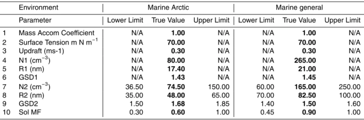
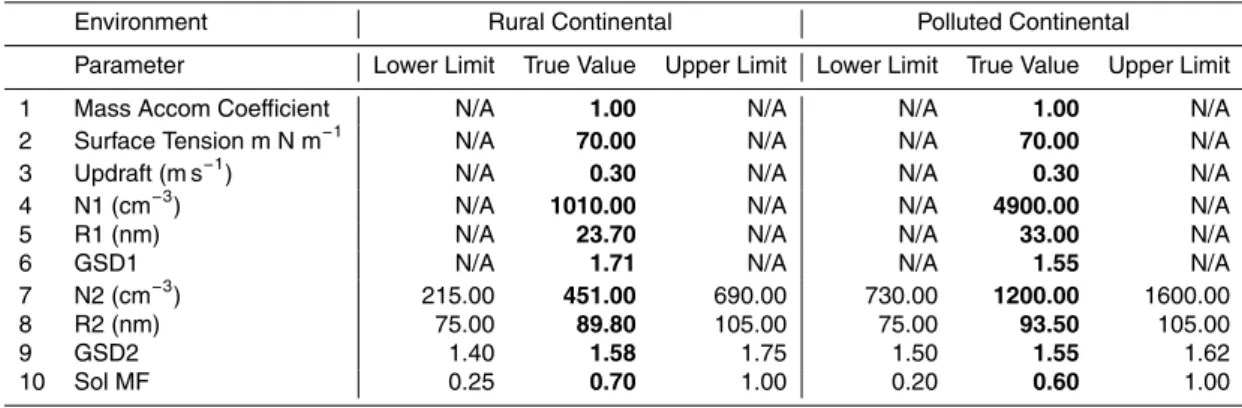
The base value for all 10 input parameters of the pseudo-adiabatic cloud parcel model and the associated lower and upper limits for the four parameters to be optimised can be found in Table 1 for marine Arctic and marine general conditions; in Table 2 for ru-ral continental and polluted continental environments. For each aerosol environment the base value, and lower/upper bounds for the lognormal parameters describing the 15

accumulation mode were obtained using the statistics from P. Tunved, personal com-munication, 2011; Heintzenberg et al., 2000; Tunved et al., 2005; and Birmili et al., 2001 as a guide. The aerosol size distributions for marine Arctic, and marine general environments used to generate the synthetic CDNC distribution data can be found in P11. The base soluble mass fraction and upper and lower limits are selected based 20

on values from the literature (P11). The only diff_{erence to P11 is that we constrain the}

(14)

ACPD

11, 20051–20105, 2011

Title Page

Tables Figures

◭ ◮

Back Close

Full Screen / Esc

Discussion

P

a

per

|

Dis

cussion

P

a

per

|

Discussion

P

a

per

|

Discussio

n

P

a

per

|

Synthetic calibration data

To benchmark our MCMC algorithm, it is useful to start the inverse modelling analysis with numerically generated cloud data (i.e. “synthetic” calibration data) simulated using known values of the model parameters. This is important to ensure that the subsequent sensitivity analysis is not contaminated by model error or parameter non-identifiability 5

The choice of the calibration data set essentially determines the posterior distribution of the parameters. More information available in the calibration data allows for more parameters to be constrained. On the contrary, noisy data with poor sensitivity to the individual parameters will result in uncertainty in the posterior distribution. Hence, in such situations it will be diffi_{cult to reduce parameter uncertainty, and appropriately}

10

calibrate the pseudo-adiabatic cloud parcel model. Thus, the information content of the calibration data directly determines the identifiability, uncertainty, and correlation of the pseudo-adiabatic cloud parcel parameters (P11).

The main thrust of this paper is to assess the impact of the calibration parameters on the number of activated cloud droplets and we therefore remove the interstitial aerosols 15

from our calibration data set. This droplet size distribution is output at 100 m above cloud base as the calibration target.

To investigate the influence of environmental conditions on the posterior distribution and sensitivity of the governing pseudo-adiabatic cloud parcel model parameters we synthetically generate CDNC distributions using input from four different aerosol envi-20

ronments (cf. Sect. 2.4). The resulting CDNC distributions are depicted in Fig. 1.

2.5 Coupling pseudo-adiabatic cloud parcel model to MCMC algorithm

Figure 2 provides a schematic overview of the cloud-parcel parameter estimation prob-lem using MCMC simulation with DREAM. The plot is essentially divided in two main parts. The top part corresponds to “the real-world” (in our case represented by synthet-25

(15)

ACPD

11, 20051–20105, 2011

Title Page

Tables Figures

◭ ◮

Back Close

Full Screen / Esc

Discussion

P

a

per

|

Dis

cussion

P

a

per

|

Discussion

P

a

per

|

Discussio

n

P

a

per

The terminology “true” and “observed” response is used to diff_{erentiate between}

re-ality and respective observations of rere-ality that are prone to measurement error and uncertainty. Our framework thus explicitly recognizes the role of measurement error. The DREAM algorithm is now used to find those values of the pseudo-adiabatic cloud parcel parameters that provide the best possible fit to the measured droplet size dis-5

tribution. This results in an ensemble of parameter values that define the posterior distribution.

Mathematically, the model calibration problem can be formulated as follows: Let ˆ

Y_φ₍_x,θ₎=_{y˜₁,...,y˜_n}denote predictions of the modelΦwith observed input variables

X and model parametersθ. Let,Y =_{_y,...,y_n_}_represent_n_{observations of the droplet}

10

size distribution. The diff_{erence between the model-predicted and measured droplet}

size distribution can be represented by the residual vectorE _as:

E₍_θ₎=_G_{( ˜}_Y₎₋_G₍_Y₎=_{_G_{( ˜}_y₁₎₋_G₍_y₁₎_,...,G_{( ˜}_y_n₎₋_G₍_y_n₎_}=_{_e₁₍_θ₎_,...,e_n₍_θ₎_} ₍₂₎

whereG(.) allows for various monotonic (such as logarithmic) transformations of the output. The inverse modeling approach now relies on the estimation of the set of input 15

parametersθ such that the measureE_{, commonly called the objective function (OF),} is in some sense forced to be as close to zero as possible.

We run the DREAM algorithm with the parameter bounds listed in Table 1 and with 10 diff_{erent Markov chains and 75 000 cloud parcel model evaluations. Our experience}

with other parameter estimation problems of similar dimension suggests that these set-20

(16)

ACPD

11, 20051–20105, 2011

Title Page

Tables Figures

◭ ◮

Back Close

Full Screen / Esc

Discussion

P

a

per

|

Dis

cussion

P

a

per

|

Discussion

P

a

per

|

Discussio

n

P

a

per

|

2.6 Defining the Objective Function (OF)

The most popular OF is the simple least squares (SLS) or maximum likelihood estima-tor. We follow this assumption and use the following definition of the OF:

OF=

n

X

i=₁

w_i[y_i−Φ₍_X_i_,θ_)]2=

n

X

i=₁

w_ie_i(θ)2 (3)

Theθvector consists of calibration parameters, for the cloud-aerosol inverse problem 5

these are the input lognormal parameters describing the accumulation mode and sol-uble mass fraction, whereas thew_i denote weights associated with a particular mea-surement point. In this study in which we use a synthetically generated calibration dataset we assume the weights of the individual data points in Eq. (3) are similar and equal to one.

10

The identifiability of calibration parameters is highly dependent on the definition of the OF. Adiabatic cloud parcel models that employ a moving centre (MvCr) framework are particularly problematic for inverse modelling techniques as both the droplet radius and number are simultaneously changing in each run (P11).

For comparisons between diff_{erent simulations to be meaningful, it is essential to}

15

construct a calibration data set that is constant with respect to the droplet size grid regardless of the prescribed calibration input parameters. If the OF is defined using only the raw MvCr output of the d N/dlogD_p function, without any radius information, then it is in theory possible to achieve exactly the same function shape for diff_erent

parameter combinations, i.e. the calibration parameters are non-identifiable. 20

To avoid this, a direct interpolation of the droplet size distributions (Fig. 1) is per-formed so that the corresponding model predictions of the d N/dlogD_p size distribu-tion funcdistribu-tion, ˆY =_{y˜₁,...,y_n} are interpolated to the size grid of the calibration data, Y =_{_y₁_,...,y_n_}_{. Unfortunately this interpolation (termed “interpolation method” herein)}

results in poorly defined and chaotic response surfaces (P11) which result in non-25

(17)

ACPD

11, 20051–20105, 2011

Title Page

Tables Figures

◭ ◮

Back Close

Full Screen / Esc

Discussion

P

a

per

|

Dis

cussion

P

a

per

|

Discussion

P

a

per

|

Discussio

n

P

a

per

current definition of the calibration data we are restricted to studying only four pa-rameters or the algorithm struggles to locate the calibration parameter values used to generate our calibration data for the perfect case (no measurement error).

In reality neither the adiabatic cloud model nor the measurements are perfect. There-fore, in order to investigate parameter sensitivity when using a synthetically generated 5

calibration data set, it is necessary to corrupt the calibration data with a “measure-ment error”, (Koda and Seinfeld, 1978). This is done in the following manner: First an error fraction is defined as 10 % of the calibration data, and thus a sigma vector, σ_, representing a synthetic variability is calculated as:

σ=₀_.₁₀_·Y_, ₍₄₎

10

where the error is then defined from thisσ using the Matlabnormrnd function as:

Y

error=normrnd(µ,σ,NY) (5)

whereN_Y denotes the number of observations (cloud model size bin resolution) used to calibrate the cloud-parcel model. Thenormrnd function generates random numbers from the normal distribution with mean parameterµ=_{0 and standard deviation}_σ_{. To}

15

obtain our corrupted calibration data, the calibration data vector is corrupted with this measurement error vector by.

Y =Y +Y

error (6)

The simulation is then re-run to obtain the parameter sensitivity from the posterior distribution. This is calculated by allowing an 80 % burn in (cf. Sect. 2.2) of the MCMC 20

simulation (i.e. we only take the last 20 % of the simulations at which point the algorithm has reached a stationary posterior distribution).

The algorithm was run first with no measurement error to be sure of convergence and then again with the calibration data corrupted with a synthetic measurement error (Eq. 4–6) to obtain parameter uncertainty.

(18)

ACPD

11, 20051–20105, 2011

Title Page

Tables Figures

◭ ◮

Back Close

Full Screen / Esc

Discussion

P

a

per

|

Dis

cussion

P

a

per

|

Discussion

P

a

per

|

Discussio

n

P

a

per

|

3 Results

3.1 Performed sensitivity simulations and analysis

In this first study using DREAM we limit ourselves to investigating four parameters when using the “Interpolation method” for the OF definition. Thus, simulations and analysis will be presented for the calibration parameters deemed to be of most interest. Those 5

are the number concentration, mean radius, and geometric standard deviation of the accumulation mode as well as the soluble mass fraction (cf. Tables 1–2). The analysis is performed for four aerosol environments (Sect. 2.4)

In the following, we will:

1. Show that MCMC simulation with DREAM converges nicely to the known param-10

eter values (in the case of synthetic data) used to create the synthetic (artificial) data for marine general and rural continental aerosol environments.

2. Perform an initial sensitivity analysis of the calibration input parameters for marine general and rural continental environments.

3. Examine the posterior parameter distributions for all four aerosol environments in 15

order to present a more detailed sensitivity analysis whilst concurrently revealing the eff_{ects of parameter compensation within the adiabatic cloud parcel model.}

4. Repeat step 3 for a “low” and “high” updraft velocity to study the eff_{ect of updraft}

velocity on the derived sensitivity.

3.2 Performance of MCMC algorithm

20

In order to make sure that the MCMC algorithm can successfully find the true optimal solution (RMSE=_{0) for every calibration parameter for the “perfect case” (no}

(19)

ACPD

11, 20051–20105, 2011

Title Page

Tables Figures

◭ ◮

Back Close

Full Screen / Esc

Discussion

P

a

per

|

Dis

cussion

P

a

per

|

Discussion

P

a

per

|

Discussio

n

P

a

per

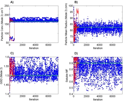
and Fig. 4 for marine general and rural continental data, respectively. The success of the MCMC algorithm in reaching the true synthetic calibration input parameter values is illustrated by the convergence of the Markov Chains (red lines) during the length of the simulation towards the true values (green dotted line). It is clear that when the size distribution measurements are not corrupted with a synthetic measurement error the 5

single true optimal solution for every parameter is successfully located in fewer than 40 000 function evaluations.

The results from subsequent simulations in which we corrupted our calibration data with a 10 % synthetic measurement error were overlaid for each aerosol environment onto Figs. 3 and 4 respectively with blue dots so that the sensitivity bounds with re-10

spect to the true optimal solution are visible. The range on theY-axis of each subplot in Figs. 3 and 4 corresponds to the prior range defined in Tables 1, 2 for marine general and rural continental conditions within which the algorithm is allowed to search. This means that the range of the posterior distribution (last 15 000 simulations) for a spe-cific parameter in relation to the prior distribution (seen at iteration=_{0) provides key}

15

information as to how sensitive the particle size distribution is to changes in a param-eter. Since all input parameters are simultaneously optimised within this framework, a parameter whose posterior distribution has a small spread about the true solution is of high importance; as there are few combinations for which it can be defined in the model input and still get a measurement output which is close to the calibration data. 20

In order to visualise the convergence of the individual Markov Chains to the optimal solution we illustrate the evolution of the OF during the MCMC simulation in Fig. 5 for one parameter, the soluble mass fraction, for marine general conditions. This param-eter creates some diffi_{culties for the search algorithm as the convergence is not rapid.}

This can be explained by the fact that it is possible to achieve the same closeness of 25

fit between the generated data set and the calibration data set (RMSE) for diff_erent

(20)

ACPD

11, 20051–20105, 2011

Title Page

Tables Figures

◭ ◮

Back Close

Full Screen / Esc

Discussion

P

a

per

|

Dis

cussion

P

a

per

|

Discussion

P

a

per

|

Discussio

n

P

a

per

|

3.3 Sensitivity analysis

3.3.1 Initial results from optimisation procedure

The parameter sensitivity is explored by corrupting our calibration data set with a syn-thetic measurement error (Eqs. 3–5).

Based on the width of the posterior distribution (cf. Sect. 3.2) it is clear from Figs. 3a 5

and 4a that for both aerosol environments the key calibration parameter for describing the CDNC distribution is the number of particles in the accumulation mode, as its pos-terior range is the narrowest out of all calibration parameters relative to its prior range. Conversely for marine general conditions these figures indicate that the least impor-tant calibration parameter for our pseudo-adiabatic cloud parcel model is the soluble 10

mass fraction. For rural continental conditions the diff_{erence between the widths of the}

posterior distributions is less clear.

The CDNC distribution associated with this posterior distribution is shown in Fig. 6 for all four aerosol environments. It is clear that the solutions stored within the posterior distribution bound the calibration data set for all aerosol conditions.

15

In order to confirm these preliminary indications and see the true relative sensitiv-ity between diff_{erent calibration parameters we normalise the posterior ranges by the}

prior ranges for each individual parameter. The last 20 % of the samples generated with DREAM are considered, thus a burn-in of 80 %. Burn-in is required to give the MCMC sampler time to converge to the posterior distribution. For our simulations this 20

results in the last 15 000 parameter combinations stored in the individual chains. These parameter values correspond to the stationary distribution of the calibration parameters and can be used to define parameter and predictive sensitivity.

3.3.2 Parameter sensitivity

We will now explore the relative sensitivity between the parameters by investigating 25

(21)

ACPD

11, 20051–20105, 2011

Title Page

Tables Figures

◭ ◮

Back Close

Full Screen / Esc

Discussion

P

a

per

|

Dis

cussion

P

a

per

|

Discussion

P

a

per

|

Discussio

n

P

a

per

aerosol environments (Fig. 7). A larger normalised posterior range represents smaller sensitivity to a calibration parameter. It should be noted here that our normalised ranges used to infer parameter sensitivity are dependent on the prior range. It is for this reason that the prior ranges have to represent physically reasonable lower and upper limits for each parameter (cf. Sect. 2.4).

5

The results for marine general aerosol conditions (Fig. 7b) confirm those displayed in Fig. 3, i.e., for the pseudo-adiabatic cloud parcel model used in this study the particle concentration of the accumulation mode is the most important parameter for the acti-vation of cloud droplets. The geometric standard deviation of the accumulation mode and soluble mass fraction are least important. For marine Arctic conditions (Fig. 7a) 10

the results are similar; however, the geometric standard deviation is of larger impor-tance. This low sensitivity to chemistry in clean CCN limited environments is intuitive; it does not matter how soluble a particle is if it does not exist. Thus, the number of particles must be, up to a certain threshold the limiting factor in any environment for the cloud droplet nucleating ability of an aerosol population. This will be especially true 15

for environments in which the number of available cloud condensation nuclei (CCN) is limited (P11). This is also consistent with current observations and theory for cleaner environments (e.g. Dusek et al., 2006).

For rural continental conditions, the overall picture is the same, the number of aerosol particles in the accumulation mode is still the key parameter and the soluble mass 20

fraction is the least important calibration parameter (Fig. 7c). However, now the solu-ble mass fraction is relatively more important. The geometric standard deviation is of equal importance as the mean radius, and there is a dramatic increase in the accu-mulation mode number normalised posterior range compared to marine general condi-tions. Moving to a yet further polluted environment (Fig. 7d) we see a shift in the domi-25

nant parameter for describing droplet activation to the parameter representing particle chemistry, with the diff_{erence between sensitivity of the lognormal aerosol}

(22)

ACPD

11, 20051–20105, 2011

Title Page

Tables Figures

◭ ◮

Back Close

Full Screen / Esc

Discussion

P

a

per

|

Dis

cussion

P

a

per

|

Discussion

P

a

per

|

Discussio

n

P

a

per

|

is relatively low, (0.3 m s−1). For more polluted aerosol conditions with a low updraft velocity the higher concentration of larger particles results in the activation of larger droplets, followed by a suppression of peak supersaturation which tends to reduce the total number of droplets activated. This allows for the soluble mass fraction to be rel-atively more important, in agreement with previous studies (Feingold, 2003; Lance et 5

al., 2004; Ervens et al., 2005; Quinn et al., 2008). It is expected at higher updraft velocities a greater fraction of the larger aerosol would be able to achieve the critical supersaturation required for activation (regardless of composition), thereby decreasing the relative sensitivity of the aerosol composition compared to aerosol size (Antilla and Kerminen, 2007).

10

The evolution of the calibration parameter sensitivity from very clean (marine Arctic) to more polluted conditions is in keeping with our two dimensional response surface analysis of the sensitivity between number and chemistry (P11). This is caused by the shift from CCN limited to CCN saturated environments and the associated competition for water vapour. Also similar to P11 for which the updraft was relatively low, there is a 15

clear tipping point in the calibration parameter sensitivity between marine general and rural continental conditions (Fig. 7).

For low updraft velocities (0.3 m s−1) the chemistry appears to be of similar impor-tance to the accumulation mode mean radius for rural continental conditions, and more important than the accumulation mode mean radius for polluted continental conditions. 20

This result highlights the importance of accurately representing the chemical compo-sition of aerosols. For rural continental conditions the geometric standard deviation of the accumulation mode is only slightly less important for the cloud nucleating ability of particles than the mean radius. This is in agreement with the study of Antilla and Kerminen (2007).

(23)

ACPD

11, 20051–20105, 2011

Title Page

Tables Figures

◭ ◮

Back Close

Full Screen / Esc

Discussion

P

a

per

|

Dis

cussion

P

a

per

|

Discussion

P

a

per

|

Discussio

n

P

a

per

3.4 Distribution of parameter values

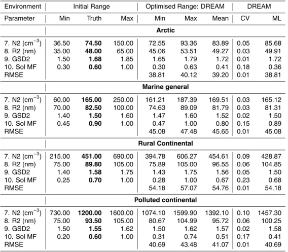
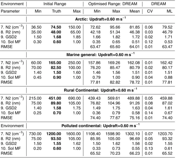
Table 3 lists values of the derived posterior mean, minimum, maximum, coefficient of variation (CV) and maximum likelihood (ML) value of the four input parameters under investigation for all four aerosol environments. The ML value is the value associated with a calibration parameter that gave the best fit to the CDNC distribution stored in the 5

calibration data. For all aerosol environments the soluble mass fraction has the highest coeffi_{cient of variation, showing the parameter to have the highest uncertainty within}

the posterior parameter distribution. Overall the minimum and maximum ranges after optimisation are generally more constrained for the two clean environments compared to the two more polluted conditions. In addition the ML of the soluble mass fraction for 10

polluted continental conditions is 0.41, considerably lower than the true value of 0.60. This indicates that for polluted regions, more variability in the parameters describing the activation of cloud droplets is possible, whilst still achieving approximately the same CDNC distribution.

The ML value is very close to the true values of the calibration parameter for marine 15

general and rural continental conditions (Table 3; Fig. 7b). For marine Arctic and ru-ral conditions the ML value departs considerably from the true values for the soluble mass fraction (0.36 compared to 0.60). For polluted conditions the ML for the number concentration in the accumulation mode is 1457 cm−3,∼250 cm−3higher than the true value. The reason for this departure from the true value can be partially ascribed to 20

the magnitude of the corrupted calibration data. The sigma values calculated using a 10 % error in Sect. 2.6 were generally positive, meaning that the corrupted droplet size distribution on average had a higher peak droplet number than the calibration data set. Therefore, it is logical that the MCMC algorithm tends towards a ML accumulation mode number concentration that is higher than the true value for this parameter. This 25

(24)

ACPD

11, 20051–20105, 2011

Title Page

Tables Figures

◭ ◮

Back Close

Full Screen / Esc

Discussion

P

a

per

|

Dis

cussion

P

a

per

|

Discussion

P

a

per

|

Discussio

n

P

a

per

|

3.5 Parameter compensation and correlation

To explore these statistics further we derive the marginal distributions for each aerosol environment and present the results in Fig. 8. These histograms are derived by plotting the DREAM generated samples of each individual parameter. A marginal distribution that extends over the entire prior ranges is indicative for poor parameter sensitivity. On 5

the contrary, if the histogram is well defined with narrow ranges, then this parameter is well defined, and sensitive to the calibration data. The marginal density is the prob-ability distribution of the variables contained in our four dimensional inverse problem and provides us with counts of the calibration parameters values over their posterior distribution range, thus providing the shape of the posterior distribution. The scale and 10

orientation of the inferred parameter distributions provide important diagnostic informa-tion about the structure of the adiabatic cloud parcel model under investigainforma-tion.

For polluted continental aerosol conditions (subplots M-P) the histograms shows sig-nificant parameter variation across the posterior range indicating that there is a great range of possible aerosol physiochemical properties that can be considered optimal for 15

the given environmental conditions. This results in a decrease in the relative impor-tance of the aerosol parameters describing the accumulation mode distribution. The spread of the posterior distribution around the “correct” modal value for each calibra-tion parameter is generally more constrained for cleaner aerosol condicalibra-tions, especially for the lognormal aerosol parameters describing the accumulation mode. This indi-20

cates that for clean environments these parameters are particularly important for the accurate prediction of the droplet size distribution.

The shape of the marginal density distribution for each aerosol environment except marine Arctic indicates the presence of strong correlations between the four calibration parameters under investigation. For each of these three environments, many of the 25

(25)

ACPD

11, 20051–20105, 2011

Title Page

Tables Figures

◭ ◮

Back Close

Full Screen / Esc

Discussion

P

a

per

|

Dis

cussion

P

a

per

|

Discussion

P

a

per

|

Discussio

n

P

a

per

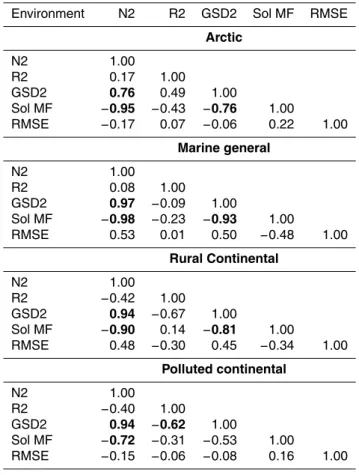
This indicates that aerosol physiochemical properties within the pseudo-adiabatic cloud parcel model compensate each other to achieve the same CDNC distribution. To examine this in more detail consider Table 4 that presents correlation coeffi_{cients of the}

samples of the posterior parameter distribution for all environments. For each aerosol environment there are three calibration parameters that show significant co-variation 5

(correlation coeffi_cient _|_r_|_>₀_._{6) which have been highlighted in bold. For all except}

the most polluted conditions the parameters show significant correlation. For instance, consider the relationship between the soluble mass fraction with both number concen-tration and geometric standard deviation of the accumulation mode, and the correlation between the number and geometric standard deviation. For the polluted continental 10

environment the correlation between the soluble mass fraction and geometric stan-dard deviation is slightly lower (0.49), there is also a stronger relationship between the mean radius and geometric standard deviation of the accumulation mode. As three of the four aerosol environments share common correlations between diff_erent

calibra-tion parameters we present these three in the form of scatter plots for all condicalibra-tions 15

(Fig. 9). These scatter plots can potentially be used to gauge at which point within the parameter space a specific parameter used to describe the activation of cloud droplets becomes important for a certain atmospheric environment. All parameter combinations present in the posterior distribution shown in Fig. 9 give approximately the same cloud droplet size distribution for each aerosol environment respectively (Fig. 6).

20

The parameter combinations in the posterior distribution for the geometric standard deviation versus the number of particles in the accumulation mode show clear pos-itive correlation for all four environments. Thus, in order to reach the same CDNC distribution it is necessary for both the number and geometric standard deviation to increase simultaneously. This is in agreement with other studies. For instance Quinn 25

(26)

ACPD

11, 20051–20105, 2011

Title Page

Tables Figures

◭ ◮

Back Close

Full Screen / Esc

Discussion

P

a

per

|

Dis

cussion

P

a

per

|

Discussion

P

a

per

|

Discussio

n

P

a

per

|

parameter space indicates the variation in sensitivity between the parameters. For the two cleaner environments, the relative importance of number increases as the geo-metric standard deviation increases; the inverse being true for the two more polluted environments. This is clearly shown by the increase in scatter for larger values of the geometric standard deviation for polluted continental conditions, and decrease for 5

marine general conditions. This analysis highlights the importance of a proper repre-sentation of the geometric standard deviation for estimating the cloud nucleating ability of particles (cf. Sect. 3.3).

There is a strong negative relationship between the soluble mass fraction and the number of aerosol particles as well as the geometric standard deviation of the accu-10

mulation mode for all aerosol environments. There is a clear shift in the linearity of the correlation as we move into polluted environments which can be attributed to the increased sensitivity of the soluble mass fraction relative to the lognormal aerosol prop-erties describing the accumulation mode. From the shape of the correlation for polluted continental conditions we can also see that the relative importance of the soluble mass 15

fraction decreases if the number or the geometric standard deviation of the accumula-tion mode is increased. This is in agreement with current theory that for more polluted environments the eff_{ect of a decrease in supersaturation with a larger geometric}

stan-dard deviation is larger in the presence of more large particles. Thus the ability for the soluble mass fraction to compensate in such conditions is reduced, evident from 20

the increase in scatter in the posterior distribution. In Fig. 10 the relationship between all four calibration parameters is presented, clearly illustrating that in order to achieve the same CDNC distribution within the parameter thresholds provided by the posterior distribution these three parameters must compensate each other so that if the soluble mass fraction is reduced both the number of particles and geometric standard deviation 25

must increase, and the mean radius of the accumulation mode must increase.

(27)

ACPD

11, 20051–20105, 2011

Title Page

Tables Figures

◭ ◮

Back Close

Full Screen / Esc

Discussion

P

a

per

|

Dis

cussion

P

a

per

|

Discussion

P

a

per

|

Discussio

n

P

a

per

The scatter plots presented in Fig. 10 illustrate that a wide range of aerosol physio-chemical properties exists that result in very similar cloud microphysical properties. Therefore, for inverse modelling of cloud-aerosol interactions detailed measurements of cloud properties are required in order for the diff_{erent clouds to be “unique”. For}

in-stance height resolved measurements, size resolved chemistry, and interstitial aerosol 5

measurements are all crucial.

In summary, the sensitivity analysis presented in Sect. 3 highlights that the size of the aerosol particle is only “sometimes” more important than its chemical composition. This must be considered in the future development of parameterisations used to calculate droplet number with respect to subsequent calculations of the aerosol indirect eff_ect,

10

thus it is paramount to estimate the importance of chemical eff_{ects for a variety of}

environments and meteorological conditions globally.

4 Effect of updraft velocity

As we cannot infer more than four parameters simultaneously given the limited informa-tion content of the data without non-identifiability contaminating our sensitivity analysis 15

(P11), we now investigate what happens with the posterior parameter distributions if the updraft is changed to 0.15 m s−1 and to 0.60 m s−1, respectively. It is important to ascertain the effect of updraft on the sensitivity of the parameters describing the aerosol physiochemical characteristics as it has a strong influence on the number and size of cloud droplets formed (Rissman et al., 2004; Brenguier and Wood, 2009). We 20

also showed from our initial response surface analysis (P11) that the CDNC distribution was most sensitive updraft perturbations.

To present the results from all updraft simulations simultaneously we calculate our relative sensitivity as 1-normalised posterior ranges for every parameter, and plot these against the accumulation mode number concentration for each aerosol environment 25