Abstract—The parallel-type neuron network (PNN) is researched to improve on the decrease in capabilities of the neuron network by the interference of the learning caused between the outputs of BP network (BPN) of two outputs or more and the difficulty of the common achievement of the middle layer used for each output. The research to compare prediction accuracies of nonlinear time series signals prediction systems using BPN and PNN has been performed so far. However, it has not attained demonstrating the existence of dominance of all prediction accuracies of PNN to BPN. Then, the experimental evaluation of the dominance of all outputs of PNN which could exist for the theory by results of the comparison of learning rules of BPN and PNN was performed using nonlinear time series signals prediction systems in this research. As a result, the dominance was showed.
Index Terms—BP Network, Learning Rule, Nonlinear Time Series Signals Prediction System, Parallel-type Neuron Network, Prediction Accuracy
I. INTRODUCTION
The parallel-type neuron network (PNN) [1]–[5] is researched to improve on the decrease in capabilities of the neuron network by the interference of the learning caused between the outputs of BP network (BPN) [6] of two outputs or more and the difficulty of the common achievement of the middle layer used for each output. It is known that causes of these problems are in the learning rule and construction of the neuron network.
To enable the learning for connection weights in middle layers of the perceptron [7], the learning rule of BPN was created with the standpoint of psychology. The inconsistence is caused between the physical events to the neuron network and the mathematics processing by the learning of BPN of two outputs or more. BPN of two outputs or more has total calculations using calculation results which are gotten independently by each output in calculations to change weights and thresholds in the last middle layer at the learning, because it has the middle layer used by each output in common. This is an origin of cause of mutual interference to the learning for each output. And, this interference back propagates one after another in the middle layers. Moreover,
Manuscript received December 30, 2008.
S. Kobayakawa is with Graduate School of Life Science and Systems Engineering, Kyushu Institute of Technology, 2-4 Hibikino, Wakamatsu-ku, Kitakyushu-shi, Fukuoka 808-0196, Japan (phone: +81-93-695-6055; fax: +81-93-695-6055; e-mail: [email protected]).
H. Yokoi is with Graduate School of Life Science and Systems Engineering, Kyushu Institute of Technology, 2-4 Hibikino, Wakamatsu-ku, Kitakyushu-shi, Fukuoka 808-0196, Japan (phone: +81-93-695-6045; fax: +81-93-695-6045; e-mail: [email protected]).
the independent learning for each output is performed only in the output layer. The research from the standpoint which the learning rule, the neuron and the network are devised has been done to improve limit of outputs accuracies of BPN caused from the problem concerning such a learning capability though BPN has approximate realization capability of an arbitrary continuous map [8], [9]. Especially, it is important to construct correctly the network which is the prime cause for this problem.
The learning rule of PNN is processed with physical events in the neuron network only one output appropriately reflected in mathematics. Furthermore, the learning only one output is performed in all layers. Therefore, it is theoretically shown that accuracies to all outputs of PNN are more dominant than ones of BPN when the learning rule of PNN is compared with one of BPN.
The research to compare the prediction accuracy has been performed about the nonlinear time series signals prediction systems using PNN and BPN from the above-mentioned viewpoint so far. However, it has not attained demonstrating the existence of dominance to BPN concerning all prediction accuracies of PNN. On the other hand, there are the detection of middle cerebral artery spasm using learning vector quantization neuron networks by M. Swiercz et al. [10] and the determining coronary artery disease and predicting lesion localization by I. Babaoglu et al. [11] in the research which applies a parallel-type of network in recent years. Then, the purpose of this research is to demonstrate the existence of domination to BPN concerning the prediction accuracies of all outputs of PNN.
II. PARALLEL-TYPE NEURON NETWORK A. I/O Characteristics
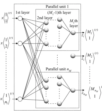
Fig. 1 shows a discrete time parallel-type neuron network (DTPNN). The neuron used for a parallel-type neuron network (PNN) can apply various types. In this research, a general artificial neuron is used for PNN. The I/O characteristics of DTPNN are shown (1) in the input layer and from (2) to (4) in the middle layers and the output layer.
( ) ( )
1 1
z x
k k
τ τ
=
(
)
1
1, 2, ,
k= " n (1)
1
( ) ( ) ( )
1
1 1
L n
i i i
j
L L L L L
u w x
k j k j k
τ τ τ
−
=
− −
=
∑
1
2, 3, ,
1, 2, , ; 1, 2, , ; 1, 2, ,
i
M L L
L M
i n j n− k n
=
⎛ ⎞
⎜ = = = ⎟
⎝ ⎠
"
" " "
(2)
Shunsuke Kobayakawa and Hirokazu Yokoi
Evaluation for Prediction Accuracies of
Parallel-type Neuron Network
Parallel unit 1 ( ) 1 1 x τ ( ) 1 2 x τ ( ) 1 1 x n τ 1 ( ) 1 1 M z τ 2 ( ) 2 1 τ M z ( ) 1 τ M M n n M z Parallel unit nM 1st layer
2nd layer
(M1-1)th layer M1th layer
Fig. 1 Discrete time parallel-type neuron network
( ) ( ) ( )
i i i
L L L
s u h
k k k
τ τ τ
= −
(
L=2,3,",M ii; =1, 2,",nM;k=1, 2,",nL)
(3)( ) ( )
( )
1
tan
i i i i i
L L L
z f s A s
k k k
τ τ τ
−
⎛ ⎞ ⎛ ⎞
⎜ ⎟ ⎜ ⎟
= ⎜ ⎟= ⎜ ⎟
⎝ ⎠ ⎝ ⎠
(
L=2,3,",M ii; =1, 2,",nM;k=1, 2,",nL)
(4)where the upper shows a layer number, the lower shows an element number in ‘< >’, the left row shows an element of output side, the right row shows an element of input side in tow rows mark of ‘< >’, x is an input signal, z is an output signal, w is a connection weight, u is the input weight sum, h
is a threshold, s is the input sum, f is an output function, A is the output coefficient, M is the output layer, the suffix i of each sign is a parallel unit number, τ is discrete time. Moreover, w and h are changed by the training.
B. Learning Rule
The learning rule of DTPNN is shown by from (5) to (11). The back-propagation for BP network of one output is applied to this learning rule for a parallel unit.
2 1 1 2 ⎛ ⎞ = ⎜ − ⎟ ⎝ ⎠ i
i i i
M
E y z
(
i=1, 2,",nM)
(5)( ) ( ) ( 1)
( )
1 1
1
i
i i i i
i
L L E L L
w w
j k L L j k
w
j k
τ τ τ
τ
α β
−
− ∂ −
Δ = − + Δ
− ∂
( ) ( ) ( 1)
1 1
i i i i i
L L L L
r z w
k j j k
τ τ τ
α β
−
− −
= − + Δ
1
2, 3, ,
1, 2, , ; 1, 2, , ; 1, 2, ,
i
M L L
L M
i n j n− k n
=
⎛ ⎞
⎜ = = = ⎟
⎝ ⎠
"
" " " (6)
( 1) ( ) ( )
1 1 1
i i i
L L L L L L
w w w
j k j k j k
τ+ τ τ
− − −
= + Δ
1
2, 3, ,
1, 2, , ; 1, 2, , ; 1, 2, ,
i
M L L
L M
i n j n− k n
=
⎛ ⎞
⎜ = = = ⎟
⎝ ⎠
"
" " " (7)
( ) ( ) ( 1)
( )
( ) ( 1)
i
i i i i
i
i i i i
L E L
h h
k L k
h k
L L
r h
k k
τ τ τ
τ τ τ α β α β − − ∂
Δ = − + Δ
∂
= + Δ
(
L=2,3,",M ii; =1, 2,",nM;k=1, 2,",nL)
(8)( 1) ( ) ( )
i i i
L L L
h h h
k k k
τ+ τ τ
= + Δ
(
L=2, 3,",M ii; =1, 2,",nM;k=1, 2,",nL)
(9)( ) ( ) ( ) ( ) ( ) ( ) 2 1 1 1 1 1 1 i i i i i i i i i i i M E r M s M
y z A
M s τ τ τ τ τ τ ∂ = ∂ ⎛ ⎞ ⎜ ⎟ = −⎜ − ⎟× ⎡ ⎤ ⎝ ⎠ +⎢ ⎥ ⎢ ⎥ ⎣ ⎦
(
i=1, 2,",nM)
(10)( ) 1 ( ) ( ) ( ) ( ) ( ) 2 1 1 1 1 1 L i i i n
i i i
k i L E r j L s j
L L L
A r w
k j k
L s j τ τ τ τ τ τ + = ∂ = ∂ ⎛ + + ⎞ ⎜ ⎟ = × ⎜ ⎟ ⎡ ⎤ ⎝ ⎠ ⎢ ⎥ + ⎢ ⎥ ⎣ ⎦
∑
12, 3, , 1
1, 2, , ; 1, 2, , ; 1, 2, ,
i
M L L
L M
i n j n k n+
= −
⎛ ⎞
⎜ = = = ⎟
⎝ ⎠
"
" " " (11)
where E is an evaluation function, y is a teacher signal, Δw is a changed value of connection weight, Δh is a changed value of threshold, α is a reinforcement coefficient of gradient-based method, β is a reinforcement coefficient of momentum, r is a reinforcement signal.
III. EXPERIMENT A. Method
Fig. 2 shows a nonlinear time series signals prediction system of five inputs four outputs which the output at τ+1 is obtained from the input at τ. BP network (BPN) and the parallel-type neuron network (PNN) of three layers are applied to this system. Next, the experiment to obtain each root mean square error (RMSE) is performed under conditions in Table 1. Furthermore, averages of their values are compared.
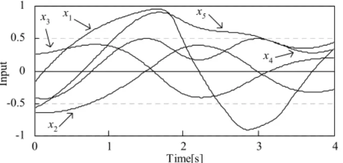
200 ms are used for the input signals and the teacher signals. The gain tuning is done as for these signals, and these values are set within the range from -1 to 1. Fig. 3 shows these signals.
Table 1 shows conditions for the evaluation experiment to their prediction accuracies. Here, initial values of the connection weights and the thresholds are decided by random numbers within the range shown in Table 1 every one time of the learning experiment. Ranges of their middle layer elements are decided for the number of elements an output to be the same about each neuron network. Moreover, αmin1 and αmin2 in Table 1 are a learning reinforcement coefficient of
x1(τ)
x2(τ)
x3(τ)
x4(τ)
x5(τ)
x1(τ+1)
x2(τ+1)
x3(τ+1)
x4(τ+1)
Inputs Outputs
System neuron network ^
^ ^
^
x1(τ+1)
+
-+
-+
-+
-x2(τ+1)
x3(τ+1)
x4(τ+1) Teacher signals
Fig. 2 Nonlinear time series signals prediction system of five inputs four outputs
-1 -0.5 0 0.5 1
Time[s]
Input
3 4
2 1
0 x1
x2
x3 x5
x4
Fig. 3 Input signals and teacher signals for the training
gradient-based method at each the minimum RMSE obtained from the rough and fine search training.
B. Results
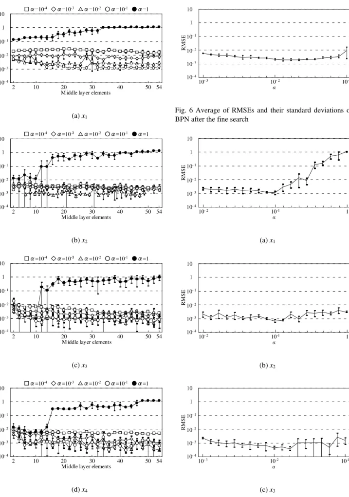
From Fig. 4 to Fig. 9 show the average RMSEs and the standard deviations of BPN and PNN which are obtained from their rough, fine and high fine search training. The length bar in these figures shows the range of the standard deviation of plus and minus. Table 2 and Table 3 show conditions at the minimum average RMSEs of BPN and PNN.
Table 1 Conditions of experiment for prediction accuracies evaluation
M iddle layer elements
RM
S
E
10- 2
10- 3
1
10- 1
10- 4
50 100 150 200
10
2 216
□α=10-4 ◇α=10-3 △α=10-2 ○α=10-4 ●α=1
Fig. 4 The average RMSEs and the standard deviations of BPN after the rough search
1/10 in the above-mentioned each interval
30,000 4 -0.3~0.3 -0.3~0.3
0 BPN
Training cycles Learning
reinforcement coefficients
Interval Range
Processing times
Learning rules Back -propagation Connection weights
Thresholds
Momentum Gradient
-based method Initial
conditions
Interval Range
PNN (1unit) Types
2~216 2 Middle layer elements
Interval Range
Learning rule for PNN
2~54
Interval Range Rough
Fine
High fine
10- 4~1
10 times 0.2αmin1~0.9αmin1
2αmin1~9αmin1 0.1αmin1, αmin1 The interval before and after
used by the fine search centering on αmin2
M iddle layer elements
RM
S
E
2 10
10 20 30
□α=10-4 ◇α=10-3 △α=10-2 ○α=10-1 ●α=1
10- 2
10- 3
1
10- 1
10- 4
40 50 54
(a) x1
M iddle layer elements
RM
S
E
2 10
10 20 30
□α=10-4 ◇α=10-3 △α=10-2 ○α=10-1 ●α=1
10- 2
10- 3
1
10- 1
10- 4
40 50 54
(b) x2
2 10
10 20 30
□α=10-4 ◇α=10-3 △α
=10-2 ○α=10-1 ●α=1
10- 2
10- 3
1
10- 1
10- 4
40 50 54
M iddle layer elements
RM
S
E
(c) x3
2 10
10 20 30
□α=10-4 ◇α=10-3 △α=10-2 ○α=10-1 ●α=1
10- 2
10- 3
1
10- 1
10- 4
40 50 54
M iddle layer elements
RM
S
E
(d) x4
Fig. 5 Averages RMSEs and their standard deviations of PNN after the rough search
α
RM
S
E
10
10- 2
10- 3
1
10- 1
10- 4
10- 3 10- 2 10- 1
Fig. 6 Average of RMSEs and their standard deviations of BPN after the fine search
α
RM
S
E
10
10- 2
10- 3
1
10- 1
10- 4
10- 2 10-1 1
(a) x1
10
10- 2
10- 3
1
10- 1
10- 4
10- 2 10-1 1
α
RM
S
E
(b) x2
α
RM
S
E
10
10- 2
10- 3
1
10- 1
10- 4
10- 3 10-2 10-1
α
RM
S
E
10
10- 2
10- 3
1
10- 1
10- 4
10- 2 10-1 1
(d) x4
Fig. 7 Averages of RMSEs and their standard deviations of PNN after the fine search
α
RM
S
E
1.0 2.0 3.0 4.0 5.0
0
0.03 0.04 0.05
×10-2
Fig. 8 Average of RMSEs and their standard deviations of BPN after the high fine search
α
RM
S
E
0.5 1.0 1.5 2.0
0
0.09 0.1 0.2
×10-2
(a) x1
α
RM
S
E
1.0 2.0 3.0 4.0
0
0.009 0.01 0.02
×10-3
(b) x2
α
RM
S
E
1.0 3.0 4.0 6.0
0
0.02 0.03 0.04
×10-3
2.0 5.0
(c) x3
α
RM
S
E
0.2 0.6 0.8 1.2
0
0.09 0.1 0.2
×10-2
0.4 1.0
(d) x4
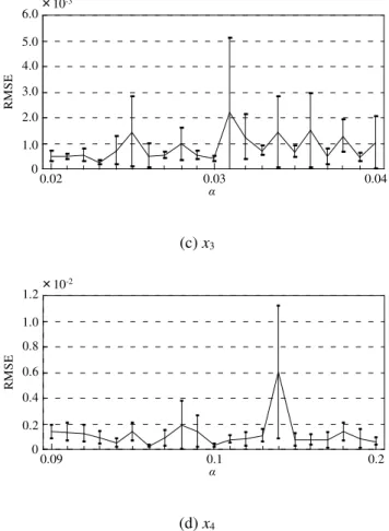
Fig. 9 Averages of RMSEs and their standard deviations of PNN after the high fine search
Table 2 Condition of BPN at the minimum average of RMSEs
Middle layer elements
Learning reinforcement coefficient
1.18×10⁻⁸
Variance RMSE
Average Waveform name
Elements an output
Standard deviation
x1 x2 x3 x4
52 13
4.0×10⁻²
1.38×10⁻³
9.18×10⁻⁴
1.09×10⁻⁴
8.57×10⁻⁴ 7.43×10⁻⁴ 6.95×10⁻⁴
8.23×10⁻⁹ 9.26×10⁻⁹ 6.32×10⁻⁸
9.07×10⁻⁵ 9.62×10⁻⁵ 2.51×10⁻⁴
Each
Table 3 Condition of PNN at the minimum average of RMSEs
Middle layer elements
Learning reinforcement coefficient
3.02×10⁻⁸
Variance RMSE
Average Waveform name
Elements an output
Standard deviation
x1 x2 x3 x4
148 37
1.4×10⁻¹
1.11×10⁻³
5.60×10⁻⁴
1.74×10⁻⁴
5.75×10⁻⁴ 2.44×10⁻⁴ 3.11×10⁻⁴
6.27×10⁻⁹ 8.36×10⁻⁹ 7.47×10⁻⁹
7.92×10⁻⁵ 9.14×10⁻⁵ 1.30×10⁻⁴
40 24 42 42
1.6×10⁻² 2.3×10⁻² 9.6×10⁻²
Each Total
Each
As a result which the minimum average RMSEs are compared, it is shown that the accuracies of all prediction
outputs of PNN are higher about each waveform in these tables than ones of BPN. Moreover, it is shown that the mean value of the minimum average RMSEs of all outputs of PNN decreases from one of BPN by 39.0 %.
IV. DISCUSSION
At the beginning, from a viewpoint of the learning rule is considered. There is (11) to calculate the reinforcement signal led from the term of gradient-based method of (6) and (8) in the last middle layer of BP network (BPN) of two outputs or more. The calculation for the amount of the product of the reinforcement signals and connection weights of all outputs of the output layer which causes the interference to the amount of change about the connection weights and the thresholds is generated in (11). This is to be changed the connection weights and thresholds in the last middle layer by other outputs which the training has not converged even if the training is converged completely by an arbitrary output. Therefore, it is thought that it is very difficult for the output which the training has been converged completely to keep the state continuously by this change. That is, this output vibrates to the teacher signal. Furthermore, this vibration has the vibrating influence to other outputs. This is the mutual interference of the learning caused between the outputs. The interferences back propagate too because the change calculations of the connection weights and the thresholds based on a reinforcement signals including this interference are executed toward the input layer one after another in the middle layers. A parallel type neuron network (PNN) does not have the above-mentioned interference, and excellent capabilities of the neuron network can be expected because it is an output a parallel unit.
Next, from the viewpoint of common for the middle layer is considered. BPN has the middle layer corresponding to each output in common. The condition to construct the middle layers prepared at each output to one, that is, the common condition of the middle layers is the case which the output signal vectors of the middle layers prepared at each output to all the input signal vectors becomes equal. This common condition of the middle layers is obviously met if a construction of coefficients of elements in the middle layers prepared at each output is equal in any middle layer. However, it is very difficult to meet such a condition actually. Therefore, BPN should have enough the learning capability to obtain the aimed output in the output layer by using an output signal vector of the last middle layer which does not satisfy the common condition of the middle layers. Such learning of BPN is like a perceptron learning only the output layer.
On the other hand, PNN has the middle layer an output to avoid the above-mentioned problem which BPN is difficult to have middle layer corresponding to each output in common. Therefore, the learning is executed in the middle layers and the output layer for the training of one output, and excellent capabilities of the neuron network can be expected.
From above two viewpoints, it is thought that all prediction accuracies of PNN are higher than ones of BPN. As a result, outputs accuracies of neuron networks for an application are ameliorable by changing BPN for PNN. Moreover, it is
thought that the outputs accuracies are more ameliorable if PNN is changed to an error convergence parallel-type neuron network system [12] which error convergence-type neuron network systems are applied to parallel units of PNN.
V. CONCLUSION
It was shown that all prediction accuracies of the parallel-type neuron network (PNN) was higher than ones of BP network (BPN), as the result of comparing the minimum average root mean square errors (RMSEs) which are obtained from nonlinear time series signals prediction systems of five inputs four outputs using BPN and PNN. Moreover, it was shown that the mean value of the minimum average RMSEs of all outputs of PNN decreased from one of BPN by 39.0 %. The future work is to perform simulation experiment of an error convergence parallel-type neuron network system which improves PNN further and to evaluate the effectiveness.
ACKNOWLEDGMENT
We wish to express our gratitude to members in our laboratory who cooperate always in the academic activity.
REFERENCES
[1] S. Kobayakawa and H. Yokoi, “The Volterra Filter Built-in Neural Network for the Aircraft Pitch Attitude Control,” Proc. of the 58th Joint
Conf. of Electrical and Electronics Engineers in Kyushu Japan, 2005, p. 429.
[2] S. Kobayakawa and H. Yokoi, “Evaluation for Prediction Capability of Parallelized Neuron Networks,” Proc. of the 8th SOFT Kyushu Chapter
Annu. Conf. Japan, 2006, pp. 3–6.
[3] S. Kobayakawa and H. Yokoi, “Application to Prediction Problem of Parallelized Neuron Networks in the Aircraft,” Technical Report of IEICE, vol. 106, no. 471, SANE2006–119–133, Jan. 2007, pp. 43–45. [4] S. Kobayakawa and H. Yokoi, “Evaluation of the Learning Capability
of a Parallel-type Neuron Network,” Proc. of the 1st International
Symp. on Information and Computer Elements 2007 Japan, 2007, pp. 43–47.
[5] S. Kobayakawa and H. Yokoi, “Experimental Study for Dominance to Accuracy of Prediction Output of Parallel-type Neuron Network,”
Technical Report of IEICE, vol. 108, no. 54, NC2008–1–10, May 2008, pp. 29–34.
[6] D.E. Rumelhart, G.E. Hinton, and R.J. Williams, “Learning Representations by Back-propagating Errors,” Nature, vol. 323, no. 6088, Oct. 1986, pp. 533–536.
[7] F. Rosenblatt, “The Perceptron: A Probabilistic Model for Information Storage and Organization in the Brain,” Psychological Review, vol. 65, no. 6, Nov. 1958, pp. 386–408.
[8] K. Funahashi, “On the Capabilities of Neural Networks,” Technical Report of IEICE, vol. 88, no. 126, MBE88–52, July 1988, pp. 127–134.
[9] K. Funahashi, “On the approximate realization of continuous mappings by neural networks,” Neural networks, vol. 2, no. 3, 1989, pp. 183–191.
[10] M. Swiercz, J. Kochanowicz, J. Weigele, R. Hurst, D. S. Liebeskind, Z. Mariak, E. R. Melhem, and J. Krejza, “Learning Vector Quantization Neural Networks Improve Accuracy of Transcranial Color-coded Duplex Sonography in Detection of Middle Cerebral Artery Spasm—Preliminary Report,” Neuroinformatics, vol. 6, no. 4, Aug. 2008, pp. 279–290.
[11] I. Babaoglu, O. K. Baykan, N. Aygul, K. Ozdemir, and M. Bayrak, “Assessment of exercise stress testing with artificial neural network in determining coronary artery disease and predicting lesion
localization,” Expert Systems with Applications, vol. 36, issue 2, part 1, Mar. 2009, pp. 2562–2566.
ERRATA
Date of modification is November 1, 2016.
Errors from line 2 from last line of p. 157 to line 1 of p. 158 are corrected as “Each 200 data of nonlinear time series signals from x1 to x4 which are obtained from motion equation
of a nonlinear plant at discrete time 20 ms are used for input signals and teacher signals of the system, respectively. 200 data of x5 is a control signal to this plant.”.