Estimation of Biomass
in a Submontane Beech High Forest in Serbia
Miloš K
OPRIVICA1– Bratislav M
ATOVI– or e J
OVIInstitute of Forestry, Belgrade, Serbia
Abstract – The analysed submontane beech forest (Fagenion moesiacae submontanum B. Jov. 1976)
is situated in Eastern Serbia (Majdan-Ku ajna, compartment 33a). Stand area is 22.7 ha. Its altitude is 410-520 m and the slope is 7–28°. Parent rock consists of dense limestone, and the soil is calcocambisol. The stand is uneven-aged, managed under group selection, with a volume percentage of beech is 97%. Other statistics of the stand are: site class II, canopy closure 0.9, mean diameter 39.4 cm, and Lorey’s mean height 31.0 m. For biomass evaluation, circular sample plots of 500 m2 size were used with the area intensity of 5%. While the aboveground biomass amounts to 337.69 tons/ha or 85.9%, belowground biomass makes 55.49 tons/ha or 14.1% of the total biomass. The proportion of timber in the aboveground biomass is 89.7%, brushwood 9.3% and leaves 1.0%. Estimation of biomass of the uneven-aged beech high forest was based on the results of investigations on European beech in Central/Western Europe.
European beech / Fagus moesiaca / uneven-aged stand / biomass / allometry
1 INTRODUCTION
Numerous studies have examined regression equations for the estimation of biomass of different species for different regions (Marklund 1987, Jenkins et al. 2003, Zianis-Mencuccini 2003, 2005, Muukkonen 2007). Many of these papers have dealt with European beech (Fagus sylvatica L.), and their results have been used to develop general allometric equations for estimating beech biomass in Central Europe (Wutzler et al. 2008). Similar investigations have been conducted in Croatia for European Beech (Fagus sylvatica L.), pedunculate oak (Quercus robur L.), common ash (Fraxinus excelsior L.) and European hornbeam (Carpinus betulus L.) (Luki – Kruži 1996). Beech has also been the subject of investigations in Greece (Zianis-Mencuccini 2003), in the Czech Republic (Cienciala 2006), in the Netherlands (Bartelink 1996) and some other countries.
Unfortunately, investigations of beech and other tree species’ biomass in Serbia are missing. Therefore, the development of suitable regression equations for estimating biomass of beech trees and stands has become a growing problem.
The aim of this investigation is to estimate the total aboveground dry biomass of an uneven-aged beech high forest, as well as the estimation of the biomass of its main components (stems, branches, foliage etc.). The belowground (root) dry biomass of the stand was also estimated.
2 STUDY AREA AND METHOD
The study area is a high forest stand of beech, situated in Eastern Serbia (stand 33a, management unit “Majdan-Ku ajna“). The stand area is 22.7 ha; its altitude is 410–520 m, while its slope is 7–28°. The prevailing aspect is north-west. Parent rock consists of dense limestone and the soil is acid brown, 40-80 cm deep calcocambisol. The stand is classified as a submontane beech forest (Fagenion moesiacae submontanum B. Jov. 1976). It is an uneven-aged high forest, manuneven-aged under group-selection, with virgin forest characteristics. Site class is II, canopy closure is 0.9, percentage of beech in the volume is 97%, stand quadratic mean diameter is 39.4 cm, and Lorey’s mean height 31.0 m. There are 274 trees per hectare, basal area is 33.4 m2, volume is 522.5 m3, and current annual volume increment is 8.6 m3/ha (Koprivica et al. 2008).
For the estimation of biomass and other components, simple systematic sampling was used. Twenty-three circular sample plots of 500 m2 were established on the area in a grid of 100 x 100 m. Diameter and height of the trees taller than 10 m were measured in all sample plots. Volume and volume increment were determined using adequate regression equations (Koprivica – Matovi 2005).
For the estimation of the total biomass of a tree and its parts (as dependent variables) diameter at breast height and tree height (as independent variables) were used. General regression equations for beech in Central Europe were used (Wutzler et al. 2008) for the calculation of the total aboveground tree biomass and for the evaluation of the biomass of tree components: stem, branches, timber (d > 7.0 cm), brushwood (d < 7.0 cm), leaves and roots. The equations were developed on the basis of extensive material collected in the beech forests of Germany, Italy, France, the Netherlands, Belgium, Switzerland, and the Czech Republic. They comprise data from thirteen studies on tree biomass. Unfortunately, not all studies investigated the biomass of all tree components, which means that the number of the trees in the sample used for obtaining regression equations was different. It ranged from 48 trees for root biomass to 350 trees for total aboveground tree biomass. Diameter at breast height of model trees ranged from 1 cm to 79 cm, total height from 2 m to 37 m, age from 8 to 173 years, site index from 18 to 46 and altitude from 23 m to 1560 m. Diameter at breast height, total height, age and site index (site class) of the trees in our investigated stand have values around the upper limit of the stated ranges.
Apart from the selected regression equations, we have tested similar regression equations for estimation of beech tree biomass, obtained in Croatia (Luki -Kruži 1996), the Netherlands (Bartelink 1996), Greece (Zianis-Mencuccini 2003) and the Czech Republic (Cienciala et al. 2005).
However, it has been concluded that these authors` equations can only be used for comparison with the results of the equations given by Wutzler et al. (2008), as the latter investigations were based on small samples of model trees (16–20) as well as on younger even-aged stands (56–114 years). Maximal diameters (35.1–62.1 cm) and heights (33.2–33.9 m) of model trees were consequently smaller.
3 RESULTS AND DISCUSSION
3.1 Tree biomass estimation
Biomass of the most important tree components was estimated by applying general regression equations for common beech tree biomass estimation (Wutzler et al. 2008). The equations are non-linear in their parameters. In all earlier investigations, parameters of non-linear equations were estimated by applying logarithmic transformation of original values of dependent and independent variables, i.e. by linearization of non-linear model, which enables the application of the least squares method (Baskerville 1972, Beauchamp-Olson 1973, Sprugel 1983, Wiant-Harner 1979). However, several authors stress the shortcomings of this parameter estimation method and the quality indicators of data fitting (Van Laar – Akca 2007, Cienciala et al. 2005, Zianis – Mencuccini 2003, Wutzler et al. 2008).
Therefore, modern investigations (Bates-Watts 1988, Cienciala et al. 2005, Wutzler et al. 2008) use the method of non–linear regression with the application of the iterative method for estimating the parameter values and quality indicators of data fitting.
The most commonly used models are general non-linear models:
m = a d b m = a (d2h)b m = a db hc
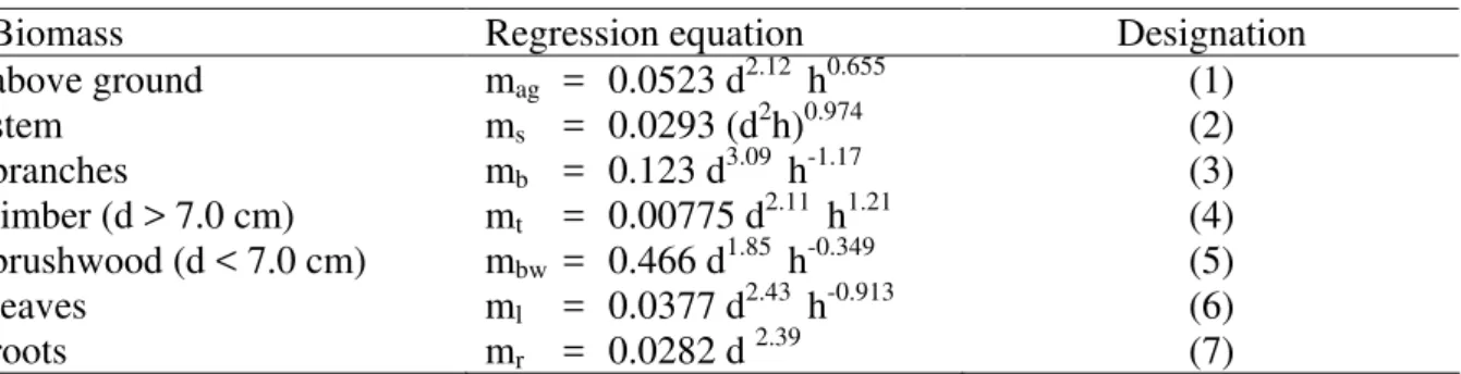
in which, biomass of a tree component (m) is a dependent variable, while diameter at breast height (d) and total tree height (h) are independent variables. Wutzler et al. (2008) used these models and developed regression equations for the estimation of tree component biomass of common beech (Table 1).
Table 1. Regression equations for estimation of tree biomass of common beech
Biomass Regression equation Designation
above ground mag = 0.0523 d2.12 h0.655 (1)
stem ms = 0.0293 (d2h)0.974 (2)
branches mb = 0.123 d3.09 h-1.17 (3)
timber (d > 7.0 cm) mt = 0.00775 d2.11 h1.21 (4)
brushwood (d < 7.0 cm) mbw = 0.466 d1.85 h-0.349 (5)
leaves ml = 0.0377 d2.43 h-0.913 (6)
roots mr = 0.0282 d 2.39 (7)
Equations of Table 1 were used to calculate biomass of all sample trees above a dbh threshold of 10.0 cm. The sample comprised 315 trees in 23 sample plots. Data processing was carried out in EXCEL programme. Total aboveground biomass was estimated in the three variants previously outlined in the study. Biomass of all trees in a sample plot was calculated as a sum of biomass of all individual trees, which was then used to estimate the biomass of the whole beech stand.
The example below illustrates the process of biomass estimation. Applying the equations of Table 1 to a tree with the diameter at breast height dbh = 39.9 cm and the total height h = 29.4 m, we obtain the following results:
– total aboveground biomass 1186.67 kg – stem biomass (stump biomass) 1036.89 kg – biomass of branches 208.42 kg – biomass of timber (d > 7,0 cm) 1106.76 kg – biomass of brushwood (d < 7,0 cm) 131.14 kg
– biomass of leaves 13.37 kg
The accuracy of the obtained results is different and dependent on the sample size (the number of model trees) and variability of the biomass components. Variant 1 provided the most accurate estimation of the total aboveground tree biomass. It was obtained by direct fitting of biomass values for all tree aboveground parts.
It would be logical to obtain the same total aboveground tree biomass by adding up biomass values for tree components. There are two possible combinations:
• total biomass = stem biomass + biomass of branches + biomass of leaves (variant 2)
• total biomass = biomass of timber + biomass of brushwood + biomass of leaves (variant 3)
However, regression equations for estimating biomass of tree components are not mutually additive. This fact has been stressed by Parresol (2001), Lambert et al. (2005) and other authors.
In the given example:
• variant 1 mag = 1186.67 kg • variant 2 mag = ms + mb + ml
mag = 1036.89 + 208.42 + 13.37 = 1258.68 kg • variant 3 mag = mt + mbw + ml
mag = 1106.76 + 131.14 + 13.37 = 1251.27 kg
Root biomass is 189.05 kg. Thus, the total tree biomass is,
mt = mag + mr
mt = 1186.67 + 189.05 = 1375.72 kg.
The proportion of the aboveground tree biomass is 86.26%, while the belowground biomass (root biomass) amounts to 13.74%.
In order to obtain more precise estimation of the biomass of the tree components, we concluded that the biomass of variant 3 was more accurate than the biomass of variant 2. There is a similar problem in the case of determining the stem volume. Therefore, the results of variant 3 were used for the estimation of the relative proportion of the biomass of components in the total aboveground tree biomass. The proportion of timber biomass is 88.45%, brushwood 10.48% and leaves 1.07%. If we apply these percentage values to the directly estimated total aboveground tree biomass, we get:
– total aboveground tree biomass 1186.67 kg biomass of timber (d >7.0 cm) 1049.61 kg biomass of brushwood (d < 7.0 cm) 124.36 kg
biomass of leaves 12.70 kg
– biomass of roots 189.05 kg
In variant 2, the proportion of stem biomass amounts to 82.38%, while the proportion of branches is 16.56% and leaves 1.06%.
The results of the selected regression equations for the estimation of common beech tree biomass (Wutzler et al. 2008) were compared with the results obtained by application of regression equations developed by other authors (Cienciala et al. 2006, Bartelink 1997, Luki – Kruži 1996, Zianis – Mencuccini 2003).
Table 2. Total aboveground beech tree biomass (d = 15–90 cm, h = 19.0–34.1 m)
Diameter (cm) 15 30 45 60 75 90
Height (m) 19.0 27.2 30.6 32.3 33.3 34.1
Tree biomass in kg
Wutzler et al. 2008 112.1 616.1 1572.0 2997.2 4907.2 7335.8 Cienciala et al. 2006 114.3 638.2 1637.2 3129.5 5131.5 7680.3 Bartelink 1997 100.1 629.4 1747.4 3543.8 6091.6 9476.6 Luki -Kruži 1996 121.4 853.0 2514.9 5313.8 9423.2 15036.6 Zianis-Mencuccini 2003 102.6 560.6 1513.8 3063.1 5291.6 8271.5
Tree biomass in %
Wutzler et al. 2008 100.0 100.0 100.0 100.0 100.0 100.0 Cienciala et al. 2006 102.0 103.6 104.1 104.4 104.6 104.7
Bartelink 1997 89.3 102.1 111.1 118.2 124.1 129.2
Luki -Kruži 1996 108.3 138.5 159.4 177.3 192.0 205.0
Zianis-Mencuccini 2003 91.6 91.0 96.3 102.2 107.8 112.7
Table 2 shows that the regression equation by Cienciala et al. (2006) comes closest to the equation given by Wutzler et al. (2008). Tree biomass estimation is 2–5% higher. The equations were developed on the basis of model trees with maximal diameter at breast height of 79 cm and height of 37 m in the second (Wutzler et al. 2008), and 62 cm diameter and 34 m height in the first equation (Cienciala et al. 2006).
The regression equations developed by the other authors show high percentage deviations, which in our opinion do not make them applicable to tree biomass estimation in high beech forests in Serbia. Applicability of the equations depends on the size range of the model trees, sample size, management practices and structure of the stands from which the tress are taken. In this particular case, maximal diameter at breast height of model trees was 35 cm and the height was up to 33 m. The data originate from well-managed 60 year-old even-aged stands.
To determine the wood density, we need to know the volume of all individual tree parts above ground. Assmann (1961) states that the average density of common beech timber is 560 kg/m3, while Cienciala et al. (2006) state that the density of beech stemwood is 575.5 kg/m3 while the density of brushwood amounts to 560.1 kg/m3. Furthermore, the Intergovernmental Panel on Climate Change (IPCC 2003) mentions 580 kg/m3 as the recommended wood density of beech trees. By using the local volume table for the whole aboveground tree (without leaves and stumps) (Mati et al. 1963) we estimated wood density is approximately 565 kg/m3.
Accurate determination of the wood density of beech trees under our site and stand conditions, requires xylometry to calculate the volume of all aboveground tree parts, while the amount of biomass can be obtained by accurate measurement of the weight of all tree parts in the dry state, i.e. by seasoning at 105 °C.
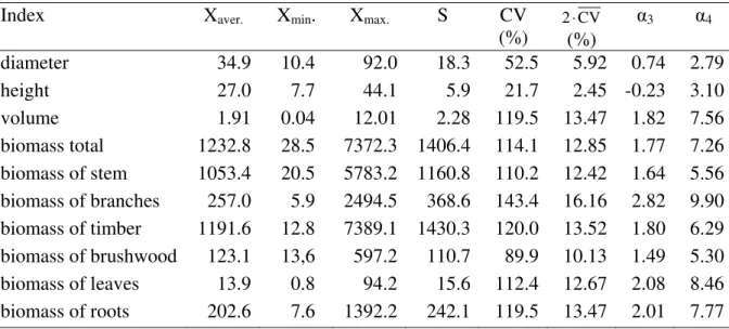
Table 3 shows the basic statistical indices of beech trees in the sample selected for the biomass estimation.
Table 3. Basic statistical indices of tree samples selected for the estimation of biomass in kg (n = 315)
Index Xaver. Xmin. Xmax. S CV
(%) 2 CV(%) ⋅
3 4
diameter 34.9 10.4 92.0 18.3 52.5 5.92 0.74 2.79
height 27.0 7.7 44.1 5.9 21.7 2.45 -0.23 3.10
volume 1.91 0.04 12.01 2.28 119.5 13.47 1.82 7.56
biomass total 1232.8 28.5 7372.3 1406.4 114.1 12.85 1.77 7.26 biomass of stem 1053.4 20.5 5783.2 1160.8 110.2 12.42 1.64 5.56 biomass of branches 257.0 5.9 2494.5 368.6 143.4 16.16 2.82 9.90 biomass of timber 1191.6 12.8 7389.1 1430.3 120.0 13.52 1.80 6.29 biomass of brushwood 123.1 13,6 597.2 110.7 89.9 10.13 1.49 5.30 biomass of leaves 13.9 0.8 94.2 15.6 112.4 12.67 2.08 8.46 biomass of roots 202.6 7.6 1392.2 242.1 119.5 13.47 2.01 7.77
3.2 Stand biomass estimation
The method described above was used to determine the total aboveground tree biomass as well as the biomass of its components for each sample plot. Tree and sample plot data were recalculated on a per hectare basis. The applied method is actually analogous to stand volume estimation.
The number of sample plots in the stand is n = 23, and the basic statistical indices are shown in Table 4.
Table 4. Basic statistical indices of the sampling in the sample plots for the estimation of stand biomass in tons per hectare (n = 23)
Index Xaver. Xmin. Xmax. S CV
(%) 2 CV(%) ⋅
3 4
number of trees 273.9 80 460 107.8 39.3 16.38 0.28 2.26
volume 522.2 298.7 875.0 163.6 31.3 13.05 0.54 2.54
biomass total 337.69 186.47 541.30 100.7 29.8 12.43 0.26 2.15 biomass of stem 288.54 153.16 454.77 66.0 29.8 12.43 0.25 2.10 biomass of branches 70.40 29.90 120.76 24.1 34.2 14.26 0.32 2.29 biomass of timber 326.41 179.90 557.87 105.3 32.2 13.43 0.47 2.46 biomass of brushwood 33.73 15.39 47.50 9.2 27.2 11.34 -0.17 2.10 biomass of leaves 3.80 1.95 5.47 1.13 29.8 12.43 0.05 1.75 biomass of roots 55.49 30.15 89.33 16.6 29.9 12.47 0.23 2.13
In this case, total aboveground tree biomass at the stand level also shows a slightly lower variation than the tree volume. Coefficient of variation is about 30%. The greatest variation is in the biomass of branches (34.2%) and the smallest is in the biomass of brushwood (27.2%). Coefficient of variation of other components ranges from 30% to 32%.
• variant 1 Mag = 337.69 tons/ha • variant 2 Mag = Ms + Mb + Ml
Mag = 288.54 + 70.40 + 3.80 = 362.74 tons/ha • variant 3 Mag = Mt + Mbw + Ml
Mag = 326.41 + 33.73 + 3.80 = 363.94 tona/ha
The biomass of the tree roots in the stand is 55.49 tons/ha.
As a result, average beech stand biomass above and below ground (roots) is most likely to be,
Mt = Mag + Mr
Mt = 337.69 + 55.49 = 393.18 tons/ha.
The proportion of the total aboveground tree biomass amounts to 85.89%, while the belowground biomass makes 14.11%.
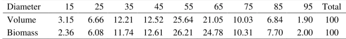
Percentage distribution of the total aboveground stand biomass by diameter classes is similar to the same distribution of its volume. To illustrate this we provide the percentage distribution of the average stand volume and biomass per hectare in Table 5.
Table 5. Percentage distribution of volume and biomass of aboveground beech stand
Diameter 15 25 35 45 55 65 75 85 95 Total
Volume 3.15 6.66 12.21 12.52 25.64 21.05 10.03 6.84 1.90 100 Biomass 2.36 6.08 11.74 12.61 26.21 24.78 10.31 7.70 2.00 100
The percentage distribution of biomass, with regard to the percentage distribution of volume by diameter classes in the stand is skewed to the greater diameter classes. However, the difference is small.
By using a simple sample, we estimated the average per hectare biomass of the investigated beech stand as well as the total biomass on the whole area of the stand.
We used the familiar formula:
m m
m t s− ⋅ < M < m t s+ ⋅ (1)
In which,
m – is average biomass per hectare in the sample,
t – is the t value from the Student distribution table - distribution for the specific probability with a degree of freedom n-1,
m
s – is the standard error of the average biomass per hectare in the sample, M – average biomass per hectare in the population (stand).
Certain components in equation (1) are calculated in the following way:
i m m
n
= , t (95% i n – 1), m m s s
n
= , i 2
m
(m m ) s
n 1 − =
− where:
mi 0 – stands for biomass per hectare for i th sample plot
Which gives
337.69 – 2.074 20.30 < M < 337.69 + 2.074 20.30
295.59 < M < 379.79
Confidence interval of the average aboveground tree biomass in the stand with 95% probability is between 295.59 and 379.79 tons/ha. Sample error is ±42.1 tons/ha or ±12.46%.
Confidence interval for the total stand biomass on the whole area (A) was calculated in the same way. The following formula was used:
m m
A(m t s ) AM (m− ⋅ < < + ⋅t s )A (2)
It follows that
22.7 295.59 < AM < 379.79 22.7
6709.89 < AM < 8621.23
Finally, the total aboveground tree biomass in stand 33a, with 95% of probability is between 6709.89 and 8621.23 tons. Sample error is ±955.67 tons or ±12.46%. We naturally assume that the area of the stand is accurately estimated. If there is an error in the estimation of the stand area, it must be taken into consideration (Mati 1977, Van Laar – Akca 2007).
In an analogous way, it is possible to estimate biomass of any tree component in the stand. We provide the estimation of the tree root biomass at stand level. Average tree root biomass at stand level, with 95% probability ranges from 48.31 to 62.67 tons/ha. Sample error is ±7.18 tons/ha or ±12.94%. It follows that the total belowground biomass at stand level ranges from 1096.64 to 1422.60 tons. Sample error is ± 163.01 tons or ±12.94%.
4 CONCLUSION
Average dry biomass of the investigated beech high forest is estimated at 393.18 tons/ha. While the aboveground biomass amounts to 337.69 tons/ha or 85.9%, belowground (root) biomass makes 55.49 tons/ha or 14.1% of the total biomass. Aboveground tree biomass at stand level naturally has greater practical importance. Thus, average aboveground tree biomass of the studied stand is between 295.59 and 379.79 tons/ha, with 95% of probability. Sample error is ±42.1 tons/ha or ±12.46%. The proportion of timber in the aboveground biomass is 89.7%, brushwood 9.3% and leaves 1.0%. Furthermore, the total biomass of all trees on the whole area of the stand is estimated at 7665.56 tons, with confidence interval between 6709.89 and 8621.23 tons.
enough. Still, we believe that we have successfully estimated the dry biomass of the investigated beech stand and that this paper has raised an important scientific and professional issue in Serbian forestry.
REFERENCES
ASSMANN, E. (1961): Waldertragskunde. BLV Velagsgesellschaft, Munchen–Bonn–Wien.
BARTELINK, H.H. (1997): Allometric relationships for biomass and leaf area of beech (Fagus sylvatica L).
Ann. Sci. For. 54: 39–50.
BASKERVILLE, G.L. (1972): Use of logarithmic regression in the estimation of plant biomass. Can. J. For. Res. 2: 49–53.
BATES, D.M. – WATTS, D.G. (1988): Nonlinear regression analysis and its applications. Wiley, New York.
BEAUCHAMP, J.J. – OLSON, J.S., (1973): Corrections for bias in regression estimates after logarithmic transformation, Ecol. 54: 1403–1407.
CANNELL, M.G.R. (1983): World forest biomass and primary production data. Academic Press, London, 391 p.
CIENCIALA, E. – CERNY, M. – APLTAUER, J. – EXNEROVA, Z. (2006): Biomass functions applicable to European beech. J. For. Sci. 51: 147–154.
HAKKILA, P. (1989): Utilization of Residual Forest Biomass. Springer, Berlin, 568 p.
JENKINS, J.C. – CHOJNACKY, D.C. – HEATH, L.S. – BIRDSEY, R.A. (2003): National-scale biomass
estimators for United States tree species. For. Sci. 49: 12–35.
JOOSTEN, R. – SCHUMACHER, J. – WIRTH, C. – SCHULTE, A. (2004): Evaluating tree carbon
predictions for beech (Fagus sylvatica L.) in western Germany. For. Ecol. Manag. 189: 87–96.
KAUPPI, P.E. – MIELIKAINEN, K. – KUUSELA, K. (1992): Biomass and carbon budget of European
forests, 1971 to 1990. Science 256: 70–74.
KÖRNER, C. – FARQUHAR G.D. – ROKSANDIC S. (1988): A global survey of carbon isotope
discrimination in plants from high altitude. Oecologia 74: 623–632.
KÖRNER, C. – FARQUHAR G.D. – WANG. S.C. (1991): Carbon isotope discrimination by plants
follows latitudinal and altitudinal trends. Oecologia 88: 30–40.
KOPRIVICA, M. – MATOVI , B. (2005): Regresione jedna ine zapremine i zapreminskog prirasta
stabala bukve u visokim šumama na podru ju Srbije [Regression equations of volume and volume increment of beech trees in high forests in Serbia]. Zbornik radova Instituta za šumarstvo, Beograd, 52–53: 5–17. (In Serbian).
KOPRIVICA, M. – MATOVI , B. (2007): Varijabilitet i preciznost procene taksacionih elemenata stabla
po debljinskim klasama u visokim sastojinama bukve [Variability and accuracy of the estimate of the taxation elements of trees by thickness classes in high beech stands]. Šumarstvo, Beograd, LIX (1–2): 1–11. (In Serbian).
KOPRIVICA, M. – MATOVI , B. – MARKOVI , N. (2008): Kvalitativna i sortimentna struktura
zapremine visokih sastojina bukve u Severno Ku ajskom šumskom podru ju [Qualitative and assortment structure of high beech stand volume in Severnoku ajsko forest area]. Šumarstvo, Beograd, LX (1-2): 41–52. (In Serbian).
LAMBERT, M. C. – UNG, C. H. – RAULIER, F. (2005): Canadian national tree aboveground biomass
equations. Can. J. For. Res. 35: 1996–2018.
LISKI, J. – LEHTONEN, A. - PALOSUO, T. – PELTONIEMI, M. – EGGERS, T. – MUUKKONEN, P. –
MAKIPA, R. (2006): Carbon accumulation in Finland’s forests 1922-2004 — an estimate obtained by combination of forest inventory data with modelling of biomass, litter and soil. Ann. For. Sci. 63: 687–697.
LU, D.S. (2006): The potential and challenge of remote sensingbased biomass estimation. Int. J. Remote Sens. 27: 1297–1328.
LUKI , N. – KRUŽI , T. (1996): Procjena biomase obi ne bukve (Fagus sylvatica L.) u panonskom
dijelu Hrvatske [Estimate of common beech (Fagus silvatica L.) biomass in Pannonian Croatia].
Unapre enje proizvodnje biomase šumskih ekosustava. Znanstvena knjiga 1, Zagreb, 131–136. (In Croatian).
MARKLUND, L.G. (1987): Biomass functions for Norway spruce (Picea abies (L.) Karst.) in Sweden.
Rapporter – Skog. 43. Departmentof Forest Survey, Swedish University of Agricultural Sciences, Uppsala.
MATI ,V.–VUKMIROVI ,V.–DRINI ,P.–STOJANOVI ,O. (1963): Tablice taksacionih elemenata visokih šuma jele, smr e, bukve, bijelog bora, crnog bora i hrasta kitnjaka na podru ju Bosne [Tables of taxation elements of fir, spruce, beech, Scotch pine, black pine and sessile oak high forests in Bosnia]. Šumarski fakultet i Institut za šumarstvo i drvnu industriju u Sarajevu. Posebno izdanje, Sarajevo. 164 p. (In Serbian).
MATI , V. (1977): Metodika izrade šumskoprivrednih osnova za šume u društvenoj svojini na podru ju SR BiH. Šumarski fakultet i Institut za šumarstvo [Methodology of making forest economy plans for public forests in SR Bosnia and Herzegovina]. Posebno izdanje (12). Sarajevo, 176 p. (In Serbian).
MATI , V. (1980): Prirast i prinos šuma [Increment and forest yield]. Univerzitet u Sarajevu, Sarajevo, 351 p. (In Serbian).
MUND, M. (2004): Carbon pools of European beech forests (Fagus sylvatica) under different
silvicultural management. UniversityGoettingen, Goettingen.
MUUKKONEN, P. (2007): Generalized allometric volume and biomass equations for some tree species
in Europe. Eur. J. For. Res. 126: 157–166.
NABUURS, G.J. – SCHELHAAS, M.J. – MOHREN, G.M.J. – FIELD, C.B. (2003): Temporal evolution of
the European forest sector carbon sink from 1950 to 1999. Glob. Change Biol. 9: 152–160. PARRESOL, B.R. (2001): Additivity of nonlinear biomass equations. Can. J. For. Res. 31: 865–878.
PAYANDEH B. (1981): Choosing regression models for biomass prediction equations, For. Chron. 57:
229–232.
RAUPACH,M.R.–RAYNER,P.J.– BARRETT,D.J.–DE FRIES,R.S.– HEIMANN,M.–OJIMA,D.S.–
QUEGAN,S.–SCHMULLIUS,C.C. (2005): Model-data synthesis in terrestrial carbon observation:
methods, data requirements and data uncertainty specifications. Glob. Change Biol. 11: 378-397. SPRUGEL D.G. (1983): Correcting for bias in log-transformed allometric equations, Ecology 64,
209–210.
THURIG, E. – SCHELHAAS, M.J. (2006): Evaluation of a large-scale forest scenario model in
heterogeneous forests: a case study for Switzerland. Can. J. For. Res. 36:
VANCLAY,J.K.–SKOVSGAARD, J.P. (1997): Evaluating forest growth models. Ecol. Model. 98: 1-12.
VAN LAAR, A. – AKÇA, A. (2007): Forest Mensuration, Springer, 383 p.
WIANT H.V.J.– HARNER E.J (1979): Percent bias and standard error in logarithmic regression, For.
Sci. 25: 167–168.
WIDLOWSKI,J.-L.–VERSTRAETE,M.M.–PINTY,B.–GOBRON, N. (2003): Allometric relationships
of selected European tree species. Tech. Rep. EUR 20855 EN. EC Joint Research Centre, Ispra, Italy.
WUTZLER,T.–WIRTH,C.–SCHUMACHER,J. (2008): Generic biomass functions for Common beech (Fagus sylvatica) in Central Europe: predictions and components of uncertainty. Can. J. For. Res.
38: 1661–1675
ZIANIS,D.–MENCUCCINI,M. (2003): Aboveground biomass relationships for beech (Fagus moesiaca
Cz.) trees in Vermio Mountain, northern Greece, and generalised equations for Fagus sp. Ann.
For. Sci. 60: 439–448.