Prerequisites for modeling price and return data series for the Bucharest Stock Exchange

(1)

Prerequisites for modeling price and return data series

for the Bucharest Stock Exchange

Andrei TINCA

The Bucharest University of Economic Studies andrei@lanifex.com

Abstract.Time series data from the capital market exhibits certain qualities which invalidate the hypotheses necessary for obtaining meaningful results from statistical modeling. This paper presents some of these qualities by looking at the time series for prices and returns on the Romanian Stock Exchange. The examples are based on the price time series and return time series of the Antibiotice securities and the BET-C index. The choice of a certain security and of the stock exchange index has been made with the intention of analyzing, in the future, the correlation between these two variables, and drawing significant conclusions which can be used for forecasts.

Firstly, we will identify the empirical proprieties of the capital market, as they are described in the field research. Secondly, we will investigate the prerequisites for modeling chronological data series; these are stationary mean and variance. In the paper, the three methods are used: graphical representation, autocorrelation and the ADF test (Augmented Dickey-Fuller). For the frequent cases where the mean is not stationary, we will present the time series differentiation method, which can be used to obtain stationary values.

Lastly, we will investigate the normality of the time series through the skewness and kurtosis methods, and through the Jarque-Bera statistic. We find out a characteristic for the capital market, in that the majority of the time series for securities have non-normal distributions.

Keywords: statistical proprieties; stationarity; autocorrelation; ADF test; differentiation; skewness; kurtosis; Jaques-Bera statistic.

JEL Classification: C12, C58, E44.

REL Classification: 11B, 11E.

(2)

Introduction

The statistical analysis leads to meaningful results only if some prerequisites are satisfied, such as the normality of the data distributions, the stationarity of the mean and the variance, independence between variables, the absence of autocorrelation in residuals, etc. In the most frequent cases, the time series do not meet these conditions, and more so by the time series from the capital market. Moreover, the time series from the capital market have specific proprieties with other time series found in the economics domain.

Consequently, in order to run statistical modeling on these time series, these problems need to be corrected. To interpret correctly the evolution and the correlations between the analyzed variables, we proceed to enforcing stationarity, normality and the elimination of autocorrelation in the residuals.

In this paper we will show the proprieties of time series from the Romanian capital market, and the correction of the stationarity propriety for the security prices. The two actions (illustrating the proprieties and correcting the stationarity) will be exemplified on the security price for the company Antibiotice, and for the BET-C composite stock exchange index.

The conclusions are valid for the other Romanian security prices and indexes. In a future article we will continue investigating the statistical proprieties of the correlations between the capital markets’ variables, and we will explore the necessary adjustments in order to run an adequate statistical model.

Empirical proprieties of security prices and returns

For the illustration of these proprieties we will use the series of daily prices and returns for the security of Antibiotice (a company traded on the Romanian Stock Exchange) and BET-C (a composite index), between 17.08.2004 and 10.03.2012. Generally, the time series from the capital market is characterized by common statistical properties of stock prices and returns.

The amount of scientific research in this area is vast, starting almost half a century ago. The most notable results belong to Fama (1965), Blattberg and Gonnedes (1974), Kon (1984), Bollerslev et al. (1992), Pagan (1996), Cont (2001), Christoffersen (2003) and many others.

(3)

9

According to Cont (2001) and Christoffersen (2003), the main properties of price and return time series are as follows:

1. The absence of autocorrelations (efficient markets in weak form).

2. Thick tails for the distributions, with large values for extreme values, compared to the normal distribution.

3. Negative skewness for the distribution of returns: negative returns have larger vales than positive returns.

4. Aggregated normalization, such that the distribution of returns during longer periods better matches the normal distribution; for example, the monthly distribution of returns match the normal distribution better than the weekly returns, which, in turn, are closer to the normal distribution than the daily returns.

5. Intermittence, which means irregular explosions in the time series of volatility.

6. Volatility clustering, denoting positive autocorrelation of volatility along several time periods; very volatile items tend to cluster together.

7. Conditional thick tails, which appear even after the correction of clustering in volatility using GARCH models. However, these tails are less thick than those found in the unconditioned distribution.

8. Gradual drop in the autocorrelations of net returns determined by the time lag, which can be expressed as an exponential function, with the exponent taking values between 0.2 and 0.4.

9. Leverage effect, such that the volatility of a financial asset is generally negatively correlated with the return of that asset.

10. Positive correlation between volatility and transaction volume.

11. The mean of the daily returns is statistically insignificant because it is dominated by the standard deviation.

12. Correlations between assets vary in time, growing when the market falls, and taking extreme values during market crash.

We will illustrate these statistical proprieties, as they are useful for comparing the price time series with the returns time series.

Data and methodology

(4)

Starting from the price time series, we will investigate the series of daily returns, calculated as continuous returns as first difference of the natural logarithm for prices:

DL ,

where:

R = effective return of the security or index “i” in day “z”;

ln(Pt) = natural logarithm of the price of the security or index during day “t”; ln(Pt-1) = same, for day “t-1”.

Modeling these two time series involves the stationarity analysis of the two time series of prices and returns.

Stationarity

Stationarity describes the stability in time for the average and the variance. In a forecast, we assume that the mean and the variance have been constant in the past, and that we expect to find these values in the future.

The stationarity is proven through: 1) graphical analysis, 2) testing serial autocorrelation using correlograms, 3) testing the existence of an unit root in the time series (ADF test).

1. The graphical representation of the analyzed time series can identify a trend and consequently, the stochastic process which generates the series is non-stationary.

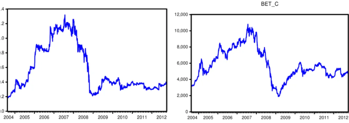
Figure 1.Graphical evolution of the ATB and BET-C prices ) ln( ) ln( ) ln( 1 1 ,      t t t t t i P P P P R 0.0 0.2 0.4 0.6 0.8 1.0 1.2 1.4

2004 2005 2006 2007 2008 2009 2010 2011 2012

ATB 0 2,000 4,000 6,000 8,000 10,000 12,000

2004 2005 2006 2007 2008 2009 2010 2011 2012

(5)

Both price time series (ATB and BET-C) have an increasing and decreasing trend, and thus are non-stationary. It is remarkable, however, that the evolution of the two price time series is almost identical.

2. The autocorrelation function is equal to k = Cov(Yt , Yt-k)/Var(Yt) and it should have k≈ 0 for all lags, if the series is stationary.

 The daily price series for ATB has the following results for the serial autocorrelation test:

Table 1.Correlations for the ATB price time series Date: 10/20/13 Time: 09:20

Sample: 8/17/2004 10/03/2012 Included observations: 2122

Autocorrelation Partial Correlation AC PAC Q-Stat Prob

|******* |******* 1 0.998 0.998 2118.6 0.000 |******* | | 2 0.997 -0.039 4231.4 0.000 |******* | | 3 0.995 0.013 6338.5 0.000 |******* | | 4 0.994 -0.005 8439.8 0.000 |******* | | 5 0.992 0.025 10536. 0.000

. . .

 The series of daily values BET-C has the following results of the same test serial autocorrelation:

Table 2.Correlations for the BET-C value time series Date: 10/20/13 Time: 09:53

Sample: 8/17/2004 10/03/2012 Included observations: 2122

|******* |******* 1 0.998 0.998 2117.1 0.000 |******* | | 2 0.996 -0.056 4226.4 0.000 |******* | | 3 0.994 -0.003 6327.8 0.000 |******* | | 4 0.992 -0.015 8421.2 0.000 |******* | | 5 0.990 0.019 10507. 0.000

. . .

(6)

autocorrelation and thus represent a random process without white noise in the residuals.

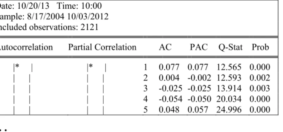
 The return time series DLATB has the following results for the serial autocorrelation test:

Table 3.Correlation for DLATB returns

Date: 10/20/13 Time: 10:00 Sample: 8/17/2004 10/03/2012 Included observations: 2121

|* | |* | 1 0.077 0.077 12.565 0.000 | | | | 2 0.004 -0.002 12.593 0.002 | | | | 3 -0.025 -0.025 13.914 0.003 | | | | 4 -0.054 -0.050 20.034 0.000 | | | | 5 0.048 0.057 24.996 0.000

. . .

 The return time series DLBET-C has the following results for the same serial autocorrelation test:

Table 4.Correlation for DLBET-C returns

Date: 10/20/13 Time: 10:02 Sample: 8/17/2004 10/03/2012 Included observations: 2121

|* | |* | 1 0.087 0.087 15.909 0.000 | | | | 2 0.005 -0.002 15.963 0.000 | | | | 3 -0.032 -0.032 18.085 0.000 | | | | 4 -0.012 -0.006 18.376 0.001 | | | | 5 0.018 0.020 19.103 0.002

. . .

In the return time series, after differentiating the returns (BLATB and DLBET-C), after the differentiation of the logarithmic series variables, the autocorrelation coefficients are close to zero for all the lags, which leads to the conclusion that these returns time series are generated by a random process (random walk, RW), and that they are, most probably, stationary.

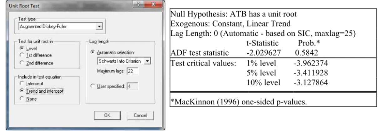
3. For the ADF test (Augmented Dickey-Fuller test statistic) it is very important to specify whether the series have a constant average and trend, which can be determined with the help of the graphical representations:

 The price time series has a constant and a trend,

(7)

 The ATB price time series has the following results for the ADF test:

Table 5. The ADF test for the ATB price time series, with constant and trend

ADF test is = – 2.029627 and is smaller in absolute value than the critical values for the usual significance levels (1% 5% 10%), which shows that the ATB price time series has a 58.42% probability to be non-stationary and possess an unit root. In order to stationarize it, we applied differentiation, which we did through logarithmic prices differentiation and obtained returns time series ATB.

 The DLATB return time series has the next results for the same ADF test:

Table 6. The ADF test for the ATB price time series (without constant and trend)

The ADF is – 42.607 and it is greater, in absolute value, than the usual significance levels of 1%, 5% and 10%, and the p-value = 0, which shows that the DLATB return series is stationary and it does not possess an unit root.

We obtain similar results for the value and return time series of the BET-C index.

Null Hypothesis: ATB has a unit root Exogenous: Constant, Linear Trend

Lag Length: 0 (Automatic - based on SIC, maxlag=25) t-Statistic Prob.*

ADF test statistic -2.029627 0.5842 Test critical values: 1% level -3.962374

5% level -3.411928

10% level -3.127864

*MacKinnon (1996) one-sided p-values.

Null Hypothesis: DLATB has a unit root Exogenous: None

5% level -1.940973

10% level -1.616599

(8)

Table 7.The ADF test for the BET-C value time series and DLBET-C time series returns Null Hypothesis: BET_C has a unit root

Exogenous: None

5% level -1.940973

10% level -1.616599

*MacKinnon (1996) one-sided p-values.

While the BET-C value time series is not stationary and has a unit root, the DLBET-C has become stationary (through differentiation) and it does not have a unit root.

With the stationarized data series we can proceed to the statistical modeling of the correlation between these variables. The results of these statistical analysis must be checked for the normality of the data series and the absence of autocorrelation between the residuals of the regression model DLATB ~ DLBET-C.

Normality

The Jarque-Bera test investigates the normality of the time series which must have skewness = 0 and kurtosis = 3 and Jarque-Bera statistics values must be very small and with p > 0. These values confirm that the series have normal distribution. To investigate the normality of the time series, we run a statistical analysis of the two price time series (ATB and BET-C), and of the returns time series resulting from these prices (DLATB and DLBET-C).

Table 8.Statistical values for price series (ATB and BET-C) and returns (DLATB and DLBET-C)

Statistics ATB BET-C DLATB DLBET-C

Mean 0.570053 5838.796 0.000305 0.000179

Median 0.396000 5365.750 0.000000 0.000000

Maximum 1.320600 10813.59 0.264304 0.105645

Minimum 0.185600 1887.140 -0.162519 -0.131168

Std. Dev. 0.316897 1914.342 0.025940 0.018453

Skewness 0.811889 0.433870 0.432202 -0.600725

Kurtosis 2.129146 2.580828 15.20034 9.711040

Jarque-Bera 300.1784 82.11072 13220.50 4107.806

Probability 0.000000 0.000000 0.000000 0.000000

Null Hypothesis: DLBET_C has a unit root Exogenous: None

5% level -1.940973

10% level -1.616599

(9)

5

From the previous table, we conclude that all the distributions of the analyzed time series exhibit positive asymmetry (skewness > 0, except for the return series of BET-C which has skewness < 0). The price distributions of ATB and BET-C are slightly platykurtic, having kurtosis < 3. However, the distributions of returns are significantly leptokuritc, having kurtosis > 3, with the series of DLATB returns exhibiting the greatest deviation from normality.

The Jarque-Bera test confirms the above: the four time series do not have normal distributions, with large values for the Jarque-Bera statistic, and thus zero probabilities for accepting the hypothesis of data distribution normality. The Jarque-Bera value for DLATB is the largest, and in consequence the series exhibits a distribution fundamentally different from the normal distribution.

The majority of the securities exhibit distributions similar to those described above. In a leptokurtic distribution, the probability of an extreme event is greater than in a normal probability (the reverse also holds). It follows that models for forecasting prices and returns will generate errors if we start from the hypothesis that their distribution is normal. Since we cannot correct the normality of these data sets, we have only to interpret the results of statistical analysis and modeling of precautionary specifying where there is an overestimation or an underesti-mation of the actual data.

Conclusions

1. Researches in the scientific literature have identified a number of empirical proprieties, specific to the capital market; these are: the lack of autocorrelations with a gradual decrease in time, thick and conditional tails of the distributions, negative asymmetry, aggregated normalization, closer to the normal distribu-tions for the series of monthly data compared to weekly data, intermittency and clusterization of volatility, negative correlation between volatility and returns, positive correlation between volatility and transaction value, and insignificance of the daily average returns and correlations between securities which vary in time during financial crises.

2. The evolution of security prices and returns exhibits these properties regardless of the value of the securities or the time period studied.

(10)

4. The stationarization of the time series is realized by differentiation on first or second degree. The differentiation of the natural logarithm of prices leads to finding out the returns, which are, generally, stationary time series.

5. Most of the securities have non-normal distributions. Because we cannot correct the non-normality of these series, we can only interpret the results of the statistical analysis and models of precautionary specifying where there is an overestimation or an underestimation of the actual data.

Note

(1)

The specificinterval in EViews would be of 2,500 observations.

References

Blattberg, R., Gonnedes, N. (1974). “A comparison of stable and Student distributions as statistical models for stock prices”, Journal of Business, Volume 47, Issue 2, pp. 244-280

Bollerslev, T., Chou, R.C., Kroner, K.F. (1992). “ARCH modeling in finance”, Journal of Econometrics, 52

Cont, R. (2001). “Empirical properties of asset returns: stylized facts and statistical issues”,

Quantitative Finance, Volume 1, Issue 2, pp. 223-236

Christoffersen, P. (2003). Elements of Financial Risk Management, San Diego, CA: Academic Press

Fama, E.F. (1965). “The Behavior of Stock-Market Prices”, The Journal of Business, Volume 38, Issue 1, pp. 34-105

Iorgulescu, F. (2012a). “The Stylized Facts of Asset Returns and their Impact on Value-at-Risk Models”, Volumul celei de a 19-a conferințe internaționale “The Persistence of the Global Economic Crisis: Causes, Implications, Solutions IECS 2012”, Sibiu, pp. 447-455

Kon, S. (1984). “Models of stock returns: a comparison”, Journal of Finance, 39