Volume , )ssue : pp.
-Available online at www.ijaamm.com ISSN: 2347-2529
Solutions of the coupled system of Burgers’ equations and
coupled Klein-Gordon equation by RDT Method
Anoop Kumar a,1 and RajanArora b
a
Department of Applied Science and Engineering, IIT Roorkee, Saharanpur Campus,Saharanpur, U.P.-247001, India
b
Department of Applied Science and Engineering, IIT Roorkee, Saharanpur Campus,Saharanpur, U.P.-247001, India
Received 15 October 2013; Accepted (in revised version) 25 November 2013
A B S T R A C T
Using the Reduced Differential Transform Method (RDTM), it is possible to find the exact solutions or better approximate solutions of wide classes of problems in mathematical physics. In this paper, this method is used for solving the coupled system of Burgers’ equations and coupled Klein Gordon Equation with given initial conditions containing arbitrary constants. The solutions obtained by RDTM are compared with the known exact solutions by fixing the arbitrary constants. The results show that the solutions obtained by RDTM are in good agreement with the known exact solutions.
Keywords: Reduced differential transform method (RDTM), the Coupled System of Burgers’ equations, the Nonlinear Coupled Klein Gordon equation, analytical and numerical solutions.
MSC 2010 codes: 35A24, 35G25, 34K28.
© 2013 IJAAMM
1 Introduction
Partial differential equations (PDEs) have numerous essential applications in various fields of science and engineering such as fluid mechanic, thermodynamics, heat transfer and physics (Debnath 1997). One of the most attractive and surprising wave phenomenons is the creation of solitary waves or solitons. Most of these equations are nonlinear partial differential equations. It is difficult to handle nonlinear part of these equations. Although most of scientists applied numerical methods to find the solution of these equations, solving such equations analytically is of fundamental importance since the existent numerical methods which approximate the solution of partial differential equations don’t result in such an exact
1
and analytical solution which is obtained by analytical methods. Hirota’s bilinear method (Hu and Wu 1998), the balance method (Wang et al. 1996), the inverse scattering method (Vakhnenko et al. 2003), the sine–cosine method (Wazwaz 2008), the homotopy analysis method (Ganji et al. 2008), the homotopy perturbation method (HPM) (He 2003, 2005), the differential transform method (DTM) (Ayaz 2003; Bildik and Konuralp 2006), the variational iteration method (VIM) (Biazar, J and Ghazvini 2007; Ganji et al. 2008; Hu and Wu 1998), Adomian’s decomposition method (ADM) (Adomian 1994; Wazwaz 2008) are some examples of analytical methods.
Recently, Keskin and Oturanç (2009) introduced a reduced form of Differential Transform Method (DTM) as reduced DTM (RDTM), and applied it to obtain solutions of non-linear PDEs and fractional PDEs (Keskin and Oturanc 2009, 2010). In this paper we have applied the reduced differential transform method (RDTM) (Keskin and Oturanc 2009, 2010) to solve the coupled nonlinear system of Burgers’ equations (Sweilam and Khader 2009) and the nonlinear coupled Klein-Gordon equation (Taghizadeh 2011). The main advantage of the method is the fact that it provides its user with an analytical approximation, in many cases an exact solution, in a rapidly convergent sequence with elegantly computed terms. The structure of this paper is organized as follows: In section 2, we begin with some basic definitions and explain the reduced differential transformation method. In section 3, we apply this method to solve the above two system of nonlinear partial differential equations.
2 The reduced differential transform method (RDTM)
The basic definitions in the reduced differential transform method (Sweilam and Khader 2009) are as follows:
2.1 Definition
Let function u(x, t) be analytic and k-times continuously differentiable with respect to time t
and space x in the domain of interest, and let
=
!
,
, (1)
where the function is the reduced differential transformation of the function , . The differential inverse transform of is defined as
, = ∑ . (2)
Then combining (1) and (2), we can write
, = ∑
! ,
. (3)
From the above definitions, it can be found that the concept of the Reduced Differential transform method is derived from the Taylor’s series expansion.
We write the gas dynamics equation in standard form
with initial condition , = , (5)
where = , , is a linear operator which has mixed partial derivatives and is a nonlinear term. According to RDTM, the iteration formula is
+ = − − , = , , , …, (6)
where and are the reduced differential transformations of the functions , and , , respectively.
Definition 2.1 implies that the initial approximation is given by the initial condition, that is
= , . (7)
Substituting in the iteration formula (6), we obtain the values of . Then the differential inverse transformation of the set of values [ ] gives approximation solution as
, = ∑
!
,
. (8)
Therefore, the differential inverse transform of is given by
, = lim → , . (9)
Authors must use Times New Roman font throughout the paper. All text, except for the title, is 12 pt. The paper title must be in Arial bold 16 pt sentence case. Leave two blank lines between the top margin and the paper title, and leave two blank lines between the paper title and the names of authors.
3 Applications
3.1 Solution of the coupled nonlinear system of Burgers’ equations
The coupled nonlinear system of Burgers’ equations (Sweilam and Khader 2009) is
− − + + = , (10)
− − + + = , (11)
subject to the following initial conditions
, = sin , , = sin . (12)
Here, = , , = , are the solutions of (10) and (11).
, = sin , (13)
, = − sin . (14)
Let us now solve the system (10) and (11) by the RDT Method.
Taking the Reduced Differential Transformation of both sides of equations (10) and (11), we obtain the iterative scheme as follows:
+ = + + , + ,
= , , , … (15)
and
+ = + + , + ,
= , , , … (16)
where is the Reduced Differential Transformation of , , is the Reduced Differential Transformation of − , , is the reduced differential transformation of − and is the reduced differential transformation of .
Using the initial conditions (12), we obtain
= , = sin , (17)
= , = sin . (18)
Now, substituting = , , , … in (15) and (16) and using (17) and (18), we obtain the following values successively
= − sin , = − sin ,
= , = ,
= − , = − ,
= , = ,
... ... ... ... ... ... ... ... ...
and so on.
, = ∑
= + + + + + ⋯
= sin − sin + − + + ⋯
= sin − + − + + ⋯
= sin .
The differential inverse transformation of the set of values [ ] gives the solution as
, = ∑
= + + + + + ⋯
= sin − sin + − + + ⋯
= sin − + − + + ⋯
= sin .
3.2 The nonlinear coupled Klein-Gordon equation
In this subsection, we will solve the nonlinear coupled Klein-Gordon equation (Taghizadeh 2011) using the RDTM.
The nonlinear coupled Klein-Gordon equation is given by
− − + + = , (19)
− − = , (20)
with initial conditions
u x, = sech[ /√ − ], (21)
v x, = − sech [ /√ − ] (22)
and
, = sech
√ tanh[√ ]. (23)
Here, = , , = , are the solutions of (19) and (20).
u x, t = ± sech[ − /√ − ] (24)
and
v x, t = − sech [ − /√ − ]. (25)
Let us now solve the system (19) and (20) by the RDT Method.
Taking the reduced differential transformation of both sides of equations (19) and (20), we obtain the iterative scheme as follows:
!
! = − + + , ,
= , , , (26)
and
+ = + , = , , , (27)
where is the reduced differential transformation of , is the reduced differential transformation of , , is the reduced differential transformation of and is the reduced differential transformation of – .
Using the initial conditions (21), (22) and (23), we obtain
U x = sech[ /√ − ],
V x = − sech[ /√ − ] ^ ,
U x = sech
√ tanh √ ,
V x = − √ + sech √ − tanh √ −
− +
sech
√ − tanh √ −
− √ − .
Also we have obtained , , and but they are not shown here since their expressions are very lengthy. In a similar way, other components may be computed.
Then, the differential inverse transformation of the set of values[ ] gives the third order approximation solution as
, = ∑
and the differential inverse transformation of the set of values [ ] gives the third order approximation solution as
, = ∑
= + + + .
4 Tables
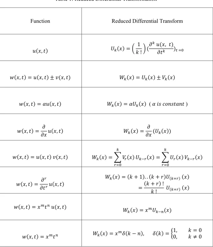
Table 1:Reduced Differential Transformation
Function Reduced Differential Transform
, = ! ,
, = , ± , = ±
, = , = ( )
, = , =
, = , , = =
, = , = + . .= ++ !
!
, = , =
Table 2: Comparison of the RDTM solution , with the exact solution (24) of the nonlinear coupled Klein-Gordon equation for = . .
t x RDTM (Taghizadeh
2011) Absolute error
0.1 -1 0 1 . . . . . . 0.00000134 0.00000401 0.00000139 0.2 -1 0 1 . . . . . . 0.00002111 0.00006380 0.00002271 0.3 -1 0 1 . . . . . . 0.00010476 0.00032085 0.00011678
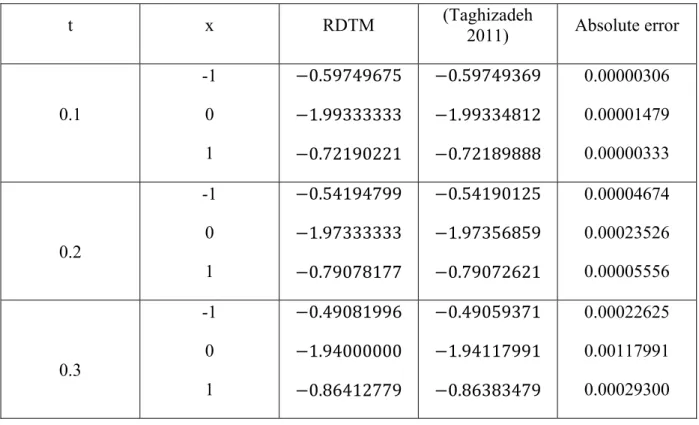
Table 3: Comparison of the RDTM solution , with the exact solution (25) of the nonlinear coupled Klein-Gordon equation for = . .
t x RDTM (Taghizadeh
2011) Absolute error
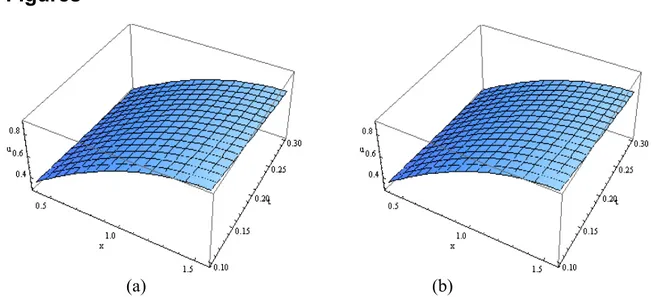
5 Figures
(a) (b)
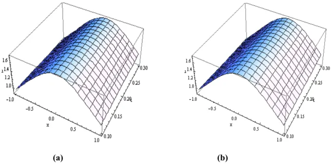
(a) (b)
Figure 2:The graph of solution , (given in (a)) in comparison with the exact analytical solution , (given in (b)).
(c) (d)
Figure 3:The graph of solution , (given in (c)) in comparison with the exact analytical solution , (given in (d)).
6 Conclusions
Klein-Gordon equation over existing numerical methods. As the method is usually tedious to use by hand, we have used the software package “MATHEMATICA” to calculate few terms of the series obtained from the RDTM. The numerical results are compared with the exact solutions in Tables 2 and 3. The solutions are also shown graphically in Figures 1, 2 and 3.
Acknowledgments
One of the authors, Mr. Anoop Kumar is highly thankful to the Ministry of human Resource Development (MHRD), New Delhi, India for the financial research grant for pursuing the Ph.D. work
References
Adomian, G. (1994): Solving frontier problems of physics: The decomposition method, Kluwer.
Ayaz, F. (2003): On the two-dimensional differential transform method, Applied Mathematics and Computation 143, pp. 361–74.
Biazar, J. and Ghazvini, H. (2007): He’s variational iteration method for solving hyperbolic differential equations. International Journal of Nonlinear Sciences and Numerical Simulation 8 (3), pp. 311–314.
Bildik, N. and Konuralp, A. (2006): The use of variational iteration method, differential transform method and Adomian decomposition method for solving different types of nonlinear partial differential equations. International Journal of Nonlinear Sciences and Numerical Simulation 7 (1), pp. 65–70.
Debnath, L. (1997): Nonlinear partial differential equations for scientist and engineers. Birkhauser, Boston.
Ganji, D. D., Sadighi, A. and Khatami, I. (2008): Assessment of two analytical approaches in some nonlinear problems arising in engineering sciences. Physics Letters A 372, pp. 4399– 4406.
He, J. H. (2003): Homotopy perturbation method: A new nonlinear technique. Applied Mathematics and Computation 135, pp. 73–79.
He, J. H. (2005): Homotopy perturbation method for bifurcation of nonlinear problems. International Journal of Nonlinear Sciences and Numerical Simulation 6 (2), pp. 207–208.
He, J.H. (1999): Variational iteration method-a kind of non-linear analytical technique: Some examples. International Journal of Non-Linear Mechanics 34 (4), pp. 699–708.
Keskin, Y. and Oturanc, G. (2009): Reduced differential transform method for partial differential equations. International Journal of Nonlinear Sciences and Numerical Simulation 10 (6), pp. 741-749.
Keskin, Y. and Oturanc, G. (2010): The reduced differential transform method: a new approach to fractional partial differential equations. Nonlinear Sci. Lett. A (1),pp. 61-72.
Liao, S. J. (2004): On the Homotopy analysis method for nonlinear problems. Applied Mathematics and Computation 147 (2), pp. 499–513.
Sweilam, N. H. and Khader, M. M. (2009): Exact solutions of some coupled nonlinear partial differential equations using the homotopy perturbation method. Computers and Mathematics with Applications 58, pp. 2134-2141.
Taghizadeh, N. (2011): Mohammad Mirzazadeh and Foroozan Farahrooz, Exact travelling wave solutions of the coupled Klein-Gordon equation by the infinite series method. AAM: Intern. J.,11(6), pp. 1964 – 1972.
Vakhnenko, V. O., Parkes, E. J. and Morrison, A. J. (2003): A Bäcklund transformation and the inverse scattering transform method for the generalized Vakhnenko equation. Chaos Solitons Fractals17 (4), pp. 683–692.
Wang, M., Zhou, Y. and Li, Z. (1996): Application of a homogeneous balance method to exact solutions of nonlinear equations in mathematical physics. Physics Letters A 216, pp. 67–75.
Wazwaz, A. M. (2002): Partial differential equations: methods and applications. The Netherlands: Balkema Publishers.