ISSN 0101-8205 / ISSN 1807-0302 (Online) www.scielo.br/cam
Two iterative algorithms for solving coupled matrix
equations over reflexive and anti-reflexive matrices
MEHDI DEHGHAN1 and MASOUD HAJARIAN2∗
1Department of Applied Mathematics, Faculty of Mathematics and Computer Science,
Amirkabir University of Technology, 424, Hafez Avenue, Tehran 15914, Iran
2Department of Mathematics, Faculty of Mathematical Sciences,
Shahid Beheshti University, G.C., Tehran 19839, Iran
E-mails: [email protected] / [email protected] / [email protected] /
[email protected] / [email protected]
Abstract. Ann×nreal matrixPis said to be a generalized reflection matrix ifPT =Pand
P2 = I (where PT is the transpose of P). A matrixA ∈Rn×nis said to be a reflexive (anti-reflexive) matrix with respect to the generalized reflection matrixPifA=P A P(A= −P A P). The reflexive and anti-reflexive matrices have wide applications in many fields. In this article, two iterative algorithms are proposed to solve the coupled matrix equations
(
A1X B1+C1XTD1=M1, A2X B2+C2XTD2=M2,
over reflexive and anti-reflexive matrices, respectively. We prove that the first (second) algorithm
converges to the reflexive (anti-reflexive) solution of the coupled matrix equations for any
ini-tial reflexive (anti-reflexive) matrix. Finally two numerical examples are used to illustrate the
efficiency of the proposed algorithms.
Mathematical subject classification: 15A06, 15A24, 65F15, 65F20.
Key words:iterative algorithm, matrix equation, reflexive matrix, anti-reflexive matrix.
1 Introduction
In this paper we use the following notation. LetRm×nbe the set of allm×nreal matrices. We use tr(A), AT,ρ(A), λ(A)andλ
max(A) to denote the trace, the
transpose, the spectral radius, the eigenvalue set and the maximum eigenvalue of the matrix A respectively. We denote by Ik and Om×n the k ×k identity matrix and them×n zero matrix, respectively. We also write them as I and
O, respectively, when the dimensions of these matrices are clear. We define an inner product ashA,Bi = tr(BTA), then the norm of a matrix Agenerated by this inner product is Frobenius norm and is denoted byhA,Ai = ||A||2.
An n×n real matrix P is said to be a real generalized reflection matrix if
PT = P and P2 = I. An n × n real matrix A is said to be a reflexive (anti-reflexive) matrix with respect to the generalized reflection matrix P if
A = P A P(A = −P A P). Rn×n
r (P)(Rna×n(P)) denotes the subspace reflexive (anti-reflexive) matrices with respect to then×n generalized reflection matrix
P. The reflexive and anti-reflexive matrices have practical applications in many areas such as the numerical solution of certain differential equations [1], pat-tern recognition [6], Markov processes [42], various physical and engineering problems [7] and so on (e.g. [20, 32, 43]). Chen [3] proposed three applications of reflexive and anti-reflexive matrices obtained from the altitude estimation of a level network, an electric network and structural analysis of trusses. The symmetric Toeplitz matrices, an important subclass of the class of symmetric reflexive matrices, appear naturally in digital signal processing applications and other areas [21].
The linear matrix equations, such as A X B = C, A X B +C X D = E and
A X B+C XTD=M, play an important role in linear system theory therefore a large number of papers have presented several methods for solving these matrix equations [2, 9, 15, 36]. Research on solving of linear matrix equations has been actively ongoing for past years. In [5], Dai studied the linear matrix equation
A X B =C, (1.1)
over symmetric matrixX. By using g-inverse, Mitra [38] obtained the common solution of simultaneous matrix equations
(
A1X B1=C1,
Navarra et al. [39] studied a representation of the solution X to the system of matrix equations (1.2). The matrix equation
A X+XTC= B, (1.3)
plays important roles in system theory, such as eigenstructure assignment [29], observer design [4], control of system with input constraint [28], and fault de-tection [30].
In [40], the necessary and sufficient condition for the existence of the solu-tion to the matrix equasolu-tion (1.3) and its solusolu-tion expression was investigated by the generalized inverse matrix. In [37], Cramer’s rules for some quaternion ma-trix equations were obtained within the framework of the theory of the column and row determinants. Kyrchei [35] considered systems of linear quaternionic equations and obtained Cramer’s rules for right and left quaternionic systems of linear equations. In [44, 45, 46], the solutions of the several generalized Sylvester matrix equations were established. In [24], a family of iterative methods for lin-ear systems is presented and a least-squares iterative solution to coupled matrix equations are studied by using the hierarchical identification principle and the star product. In [26], gradient iterative algorithms for solving Sylvester coupled matrix equations and general coupled matrix equations are studied by using the gradient search principle. In [22, 25], Ding and Chen applied a hierarchical iden-tification principle to study solving the Sylvester and Lyapunov matrix equations. Also Ding and Chen [23] proposed a hierarchical gradient iterative algorithm and a hierarchical stochastic gradient algorithm and prove that the parameter estima-tion errors given by the algorithms converge to zero for any initial values under persistent excitation. In [8, 10, 11, 12, 13, 14, 17, 18], Dehghan and Hajarian introduced some efficient iterative methods for solving Sylvester and Lyapunov matrix equations.
In this paper, we introduce two iterative algorithms, respectively, for the finding reflexive and anti-reflexive solutions of the coupled matrix equations
(
A1X B1+C1XTD1=M1,
A2X B2+C2XTD2= M2, (1.4)
(including the matrix equations (1.1)-(1.3) as special cases).
Then we study the convergence properties of the iterative algorithms. Two ex-amples verify the efficiency of the algorithms in Section 3. Section 4 concludes the paper.
2 Main results
In this section, first we give two systems of matrix equations equivalent to (1.4) over reflexive and anti-reflexive matrices, respectively. Then we will propose two efficient iterative algorithms for solving (1.4).
Lemma 2.1. The coupled matrix equations (1.4) have the reflexive solution X ∈Rnr×n(P)if and only if the system of matrix equations
A1X B1+C1XTD1= M1,
A2X B2+C2XTD2= M2,
A1P X P B1+C1P XTP D1= M1,
A2P X P B2+C2P XTP D2=M2,
(2.1)
is consistent.
Proof. First, we suppose that the coupled matrix equations (1.4) have the reflex-ive solutionX∗ ∈Rn×n
r (P). By using X∗= P X∗PandAiX∗Bi+CiX
∗T Di =
Mi, we have
AiP X∗P Bi+CiP X∗TP Di = AiX∗Bi+Ci(P X∗P)TDi
= AiX∗Bi+CiX
∗T
Di (2.2)
= Mi,
fori=1,2. It is follows from (2.2) that the reflexive matrixX∗is a solution of
the system of matrix equations (2.1).
Conversely assume that the system of matrix equations (2.1) is consistent. Let
X be a solution of the system of matrix equations (2.1). Set
e
X = X+P X P
ThereforeeX ∈Rn×n
r (P)and we can get
AieX Bi +CieXTDi = Ai
X+P X P
2
Bi+Ci
X+P X P
2
T
Di
= AiX Bi+AiP X P Bi
2 +
CiXTDi +CiP XTP Di 2
= AiX Bi+CiX
TD i
2 +
AiP X P Bi +CiP XTP Di
2 (2.4)
= Mi +Mi
2
= Mi,
fori = 1,2. Hence eX is a reflexive solution of the coupled matrix equations
(1.4). The proof is completed.
Similarly to the above lemma, we can obtain the following lemma.
Lemma 2.2. The coupled matrix equations(1.4)have the anti-reflexive solution X ∈Rna×n(P)(P 6= I ) if and only if the system of matrix equations
A1X B1+C1XTD1=M1,
A2X B2+C2XTD2=M2,
−A1P X P B1−C1P XTP D1=M1,
−A2P X P B2−C2P XTP D2=M2,
(2.5)
is consistent.
According to Theorem 4.3.8 and Corollary 4.3.10 in [33], the systems (2.1) and (2.5), respectively, are equivalent to
B1T ⊗A1+ D1T ⊗C1P(n,n)
B2T ⊗A2+ D2T ⊗C2P(n,n)
BT
1 P⊗A1P
+ DT
1P⊗C1P
P(n,n)
BT
2 P⊗A2P
+ DT
2P⊗C2P
P(n,n)
×vec(X)=vec M1,M2,M1,M2,
and
B1T ⊗A1+ D1T ⊗C1P(n,n)
B2T ⊗A2+ D2T ⊗C2P(n,n) − BT
1P⊗ A1P
− DT
1P⊗C1P
P(n,n)
− BT
2P⊗ A2P
− DT
2P⊗C2P
P(n,n)
×vec(X)=vec M1,M2,M1,M2,
(2.7)
whereP(n,n)is a permutation matrix [33]. Now by using the above results and considering Z1:=
B1T ⊗ A1+ D1T ⊗C1P(n,n)
B2T ⊗ A2+ D2T ⊗C2P(n,n)
BT
1 P⊗A1P
+ DT
1P⊗C1P
P(n,n)
BT
2 P⊗A2P
+ DT
2P⊗C2P
P(n,n) , (2.8) and
Z2:=
B1T ⊗ A1+ D1T ⊗C1P(n,n)
B2T ⊗ A2+ D2T ⊗C2)P(n,n − B1TP⊗A1P− D1TP⊗C1PP(n,n) − BT
2 P⊗A2P
− DT
2P⊗C2P
P(n,n) , (2.9)
the following lemmas are well known [31, 33, 34].
Lemma 2.3.The coupled matrix equations(1.4)have a unique reflexive solution with respect to the generalized reflection matrix P if and only if
rank((Z1,vec(M1,M2,M1,M2)))=rank(Z1)
and Z1has a full column rank. In that case, the reflexive solution of(1.4)can be expressed by the following form
X = X1+P X1P
2 where
vec(X1)=(Z1TZ1)−1Z1Tvec(M1,M2,M1,M2),
and the homogenous coupled matrix equations
(
A1X B1+C1XTD1=0,
A2X B2+C2XTD2=0, (2.11)
have a unique reflexive solution X=0.
Lemma 2.4. The coupled matrix equations (1.4)have a unique anti-reflexive solution with respect to the generalized reflection matrix P 6= I if and only if
rank((Z2,vec(M1,M2,M1,M2))) =rank(Z2)and Z2 has a full column rank. In that case, the anti-reflexive solution of(1.4)can be expressed by the following form
X = X1−P X1P
2 where
vec(X1)=(Z2TZ2)−1Z2Tvec(M1,M2,M1,M2),
(2.12)
and the homogenous coupled matrix equations(2.11)have a unique anti-reflexive solution X =0.
If Lemma 2.3 (Lemma 2.4) is applied for finding the reflexive (anti-reflexive) solution of the coupled matrix equations (1.4), we need to take the inverse of the large matrixZ1TZ1(Z2TZ2). The above method may turn out to be numerically expensive and are not practical for equations of large systems. Our purpose in this paper is to obtain two iterative methods without any inverse for solving the coupled matrix equations (1.4) over reflexive and anti-reflexive matrices. We extend the idea of the Jacobi and the Gauss-Seidel iterations to solve the coupled matrix equations (1.4) over reflexive and anti-reflexive matrices.
Suppose thatA=M−Nis a splitting of the matrixA. The Jacobi and Gauss-Seidel procedures for solving the linear systemAx =bare typical members of a large family of iterations that have the form
M x(k+1) =N x(k)+b, (2.13)
Algorithm 2.1. To solve (1.4) over reflexive matrixX:
Step 2.1.1.Input matrices A,C ∈Rr×n,B,D∈Rn×s andM∈Rr×s;
Step 2.1.2. Choose arbitrary X(1)∈ Rn×n
r (P)where P is ann-by-n arbitrary generalized reflection matrix and a parameterω∈R+;
Step 2.1.3.Calculate
Ri(1)=Mi −AiX(1)Bi−CiX(1)TDi, i =1,2;
k :=1;
Step 2.1.4.If||R1(k)|| + ||R2(k)|| =0, then stop; Else go to step 2.1.5;
Step 2.1.5.
X(k+1)=X(k)
+ω
4
2
X
i=1
ATi Ri(k)BiT +DiRi(k)TCi+P AiTRi(k)BiTP+P DiRi(k)TCiP
;
Ri(k+1)=Mi−AiX(k+1)Bi−CiX(k+1)TDi, i=1,2;
Step 2.1.6.If||R1(k+1)|| + ||R2(k+1)|| =0, then stop; Else, letk :=k+1, go to step 2.1.5.
Algorithm 2.2. To solve (1.4) over anti-reflexive matrixX:
Step 2.2.1.Input matrices A,C ∈Rr×n,B,D∈
Rn×s andM∈ Rr×s;
Step 2.2.2. Choose arbitrary X(1) ∈ Rn×n
a (P) where P 6= I is an n-by-n arbitrary generalized reflection matrix and a parameterω∈R+;
Step 2.2.3.Calculate
Ri(1)=Mi −AiX(1)Bi−CiX(1)TDi, i =1,2;
Step 2.2.4.If||R1(k)|| + ||R2(k)|| =0, then stop; Else go to step 2.2.5;
Step 2.2.5.
X(k+1)=X(k)
+ω
4
2
X
i=1
ATi Ri(k)BiT +DiRi(k)TCi−P AiTRi(k)BiTP−P DiRi(k)TCiP
;
Ri(k+1)=Mi−AiX(k+1)Bi−CiX(k+1)TDi, i=1,2;
Step 2.2.6.If||R1(k+1)|| + ||R2(k+1)|| =0, then stop; Else, letk :=k+1, go to step 2.2.5.
Now convergence properties of Algorithms 2.1 and 2.2 are presented.
Theorem 2.1. If the coupled matrix equations (1.4) have a unique reflexive solution X , then iterative solution X(k)given by Algorithm2.1converges to X for any initial reflexive matrix X(1), if the parameterωsatisfies the inequality
0< ω <2h
2
X
i=1
||Ai||2||Bi||2+ ||Ci||2||Di||2 i−1
. (2.14)
Proof. We define the estimation error matrix in the form
ε(k)=X(k)−X, for k =1,2, . . . (2.15)
By applying (2.15), we can get
Ri(k)= −Aiε(k)Bi−Ciε(k)TDi, for i =1,2, (2.16)
Also it is not difficult to obtain
ε(k+1)=ε(k)
−ω
4
2
X
i=1
h
AiTAiε(k)Bi +Ciε(k)TDi
BiT +Di
Aiε(k)Bi+Ciε(k)TDi T
Ci
+P ATi Aiε(k)Bi +Ciε(k)TDi
BiTP+P Di
Aiε(k)Bi +Ciε(k)TDi T
Now we can write
||ε(k+1)||2=trε(k+1)Tε(k+1)
= ||ε(k)||2−ω
2tr
ε(k)T
2
X
i=1
h
ATi Aiε(k)Bi +Ciε(k)TDi
BiT
+Di
Aiε(k)Bi +Ciε(k)TDi T
Ci
+P ATi Aε(k)Bi +Ciε(k)TDi
BiTP
+P Di
Aiε(k)Bi +Ciε(k)TDi T
CiP i + ω 2 16 2 X i=1 h
ATi Aiε(k)Bi +Ciε(k)TDi
BiT
+Di
Aiε(k)Bi +Ciε(k)TDi T
Ci
+P ATi Aiε(k)Bi+Ciε(k)TDi
BiTP
+P Di
Aiε(k)Bi +Ciε(k)TDi T
CiPi
2
≤ ||ε(k)||2−ω
2
2
X
i=1
trAiε(k)Bi
Aiε(k)Bi+Ciε(k)TDi T
+Ciε(k)TDi
Aiε(k)Bi+Ciε(k)TDi T
+ AiPε(k)P Bi
Aiε(k)Bi +Ciε(k)TDi T
+CiPε(k)TP Di
Aiε(k)Bi +Ciε(k)TDi T + ω 2 4 n 2 X i=1
ATi Aiε(k)Bi +Ciε(k)TDi
BiT2
+ 2 X i=1 Di
Aiε(k)Bi +Ciε(k)TDi T Ci 2 + 2 X i=1
P ATi Aiε(k)Bi +Ciε(k)TDi
BiTP
2 + 2 X i=1 P Di
Aiε(k)Bi +Ciε(k)TDi T
≤ ||ε(k)||2−ω
2
X
i=1
trAiε(k)Bi +Ciε(k)TDi
×
Aiε(k)Bi+Ciε(k)TDi T
+ω 2
2
2
X
i=1
n
||Ai||2||Bi||2+ ||Di||2||Ci||2 o
||Aiε(k)Bi+Ciε(k)TDi||2
≤ ||ε(k)||2−ωh1− ω
2
2
X
i=1
(||Ai||2||Bi||2+ ||Di||2||Ci||2) i
(2.17)
× 2
X
i=1
||Aiε(k)Bi +Ciε(k)TDi||2
≤ ||ε(1)||2−ω h
1− ω
2
2
X
i=1
(||Ai||2||Bi||2+ ||Di||2||Ci||2) i
×
k X
t=1 2
X
i=1
||Aiε(t)Bi+Ciε(t)TDi||2.
From (2.14) and (2.17), it is not difficult to get
∞
X
t=1 2
X
i=1
||Aiε(t)Bi +Ciε(t)TDi||2<∞. (2.18)
The necessary condition of the series convergence (2.18) implies that
lim t→∞
h
Aiε(t)Bi+Ciε(t)TDi i
= Ai
lim t→∞ε(t)
Bi +Ci
lim t→∞ε(t)
TD
i =0,
for i =1,2.
By considering Lemma 2.3, we have
lim
t→∞ε(t)=0.
The proof of theorem is completed.
Similar to the proof of the above theorem, we can prove the following theorem.
X for any initial anti-reflexive matrix X(1), if the parameter ω satisfies the inequality
0< ω <2h
2
X
i=1
||Ai||2||Bi||2+ ||Ci||2||Di||2 i−1
. (2.19)
Remark 2.1. The convergence factor in(2.14)and(2.19)may also be taken as:
0< ω <2
× hX2
i=1
λmax(AiATi )λmax(BiBiT)+λmax(CiCiT)λmax(DiDiT) i−1
. (2.20)
3 Numerical examples
In this section, we give two examples to illustrate the convergence of Algo-rithms 2.1 and 2.2, respectively. All the tests are performed by MATLAB.
Example 3.1. As the first example we consider the linear matrix equation
A X B+C XTD= Mwith
A=
−3.7972 0.7621 0.6154 0.4057 0.0579
0 −3.2532 0.7919 0.9355 0.3529
0 0 −3.4748 0.9169 0.8132
0 0 0 −3.6205 0.0099
0 0 0 0 −3.8103
,
B =
1 1 1 1 1
1 1 1 1 1 1 1 1 1 1
1 1 1 1 1
1 1 1 1 1 ,
C =
−4.3881 0.2259 0.2091 0 0 0.4235 −4.0637 0.3798 0.7942 0 0.5155 0.7604 −3.4846 0.0592 0.8744 0.3340 0.5298 0.6808 −4.0259 0.0150 0.4329 0.6405 0.4611 0.0503 −3.8072
D=
4.7027 −0.6979 −0.4966 −0.6602 −0.7271 0 4.9568 −0.8998 −0.3420 −0.3093 0 0 4.2523 −0.2897 −0.8385 0 0 0 4.1991 −0.5681
0 0 0 0 4.9883
, M =
118.0878 −23.1868 −53.8639 −12.1011 −52.2842
−6.3715 105.8088 −24.0695 −58.8678 9.0772
−64.4487 −13.9112 93.5506 1.4371 −69.5242 13.4263 −77.6180 16.4496 111.4427 16.3479
−36.0898 −0.8957 −51.6715 21.7130 141.3938 .
It can be verified that this matrix equation is consistent over reflexive matrices and has the reflexive solution
X∗=
−5.5945 0 3.2309 0 2.1158 0 −4.5064 0 3.8709 0 2.0000 0 −4.9497 0 3.6263
0 2.0000 0 −5.2410 0 2.0000 0 2.0000 0 −5.6207
R5×5r (P),
with P =
−1 0 0 0 0
0 1 0 0 0
0 0 −1 0 0
0 0 0 1 0
0 0 0 0 −1 .
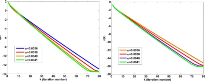
Choose arbitrary initial iterative matrixX(1)=0. By Algorithm 2.1, we obtain the sequenceX(k). In Figure 1, we report the obtained results with several values ofωwhere
δ(k)=log10||X(k)−X
∗||
||X∗|| and r(k)=log10||M−A X(k)B−C X(k)
TD||.
Figure 1 – The results of Example 3.1.
Example 3.2. Consider a pair of matrix equations in the form of (1.2) with the following parameters:
A1=
−3.7972 1.5242 1.2309 0.8114 0.1158
0 −3.2532 1.5839 1.8709 0.7057 0 0 −3.4748 1.8338 1.6263 0 0 0 −3.6205 0.0197
0 0 0 0 −3.8103
,
B1=
3.6756 0 0.6085 0.0576 0.0841 0 3.4508 0 0.3676 0.4544 0 0 3.2324 0 0.4418
0 0 0 3.0784 0
0 0 0 0 3.9943
,
A2=
5.5536 0.2259 0.2091 0 0 0.4235 5.2233 0.3798 0.7942 0 0.5155 0.7604 5.0513 0.0592 0.8744 0.3340 0.5298 0.6808 5.2317 0.0150 0.4329 0.6405 0.4611 0.0503 5.3431
B2=
−5.7027 −0.6979 −0.4966 −0.6602 −0.7271
0 −5.9568 −0.8998 −0.3420 −0.3093 0 0 −5.2523 −0.2897 −0.8385 0 0 0 −5.1991 −0.5681
0 0 0 0 −5.9883
, C1=
17.1697 −56.8568 33.5482 −25.9479 24.4829
−10.1615 15.8018 −43.9289 33.5031 −33.0153 13.4809 −12.7575 14.0869 −51.7608 15.1875
−26.6155 0.1361 −27.8120 −0.2810 −33.2835 0 −26.2971 0 −26.2605 −3.4625
, and C2=
−2.5771 −169.8176 −31.9603 −121.1339 −26.8271
−68.6326 −25.6598 −158.7006 −36.3862 −152.1132
−9.3473 −87.2429 −35.0790 −174.8441 −43.6301
−65.7124 −26.3748 −77.8285 −38.9935 −98.0133
−7.8789 −83.1321 −31.0110 −83.9174 −30.2760 .
We can verify the pair of matrix equations in the form of (1.2) are consistent over anti-reflexive matrixX and have the anti-reflexive solution
X∗ =
0 5.0484 0 3.6228 0 2.0000 0 5.1677 0 3.4115
0 2.0000 0 5.6676 0 2.0000 0 2.0000 0 2.0394
0 2.0000 0 2.0000 0
R5×5a (P).
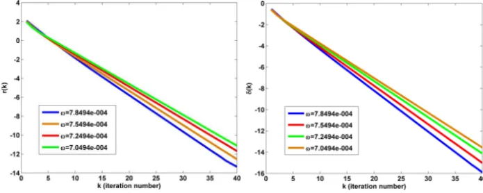
Taking X(1) = 0, we apply Algorithm 2.2 to compute X(k). The effect of changing the convergence factorωis illustrated in Figure 2 where
δ(k)=log10
||X(k)−X∗||
||X∗|| and r(k)=log10 2
X
i=1
||Ci −AiX(k)Bi||.
Figure 2 – The results of Example 3.2.
4 Concluding remarks
In this paper, we have considered the coupled matrix equations (1.4) over re-flexive and anti-rere-flexive matrices. First Algorithms 2.1 and 2.2 were intro-duced for finding reflexive and anti-reflexive solutions of (1.4). Second the convergence theorems of the iterative algorithms were presented. The exper-iments are encouraging and seem to indicate that Algorithms 2.1 and 2.2 work well for numerical examples. It is interesting to develop the introduced algo-rithms for solving other linear matrix equations. We leave it as a topic for further research.
Acknowledgements. The authors are very much indebted to an anonymous referee for his/her valuable comments and careful reading of the manuscript.
REFERENCES
[1] A. Andrew, Eigenvectors of certain matrices.Linear Algebra Appl., 7 (1973), 157–162; 455–460.
[2] A. Ben-Israel,A Cramer rule for least-norm solutions of consistent linear equa-tions.Linear Algebra Appl.,43(1982), 223–226.
[3] H.C. Chen,Generalized reflexive matrices: special properties and applications. SIAM J. Matrix Anal. Appl.,19(1998), 140–153.
[4] L. Dai, Singular Control Systems, Berlin: Springer-Vertag (1989).
[6] L. Datta and S. Morgera,Some results on matrix symmetries and a pattern recog-nition application.IEEE Trans. Signal Process,34(1986), 992–994.
[7] L. Datta and S. Morgera, On the reducibility of centrosymmetric matrices-applications in engineering problems.Circuits Systems Signal Process,8(1989), 71–96.
[8] M. Dehghan and M. Hajarian,The general coupled matrix equations over
gener-alized bisymmetric matrices.Linear Algebra Appl.,432(2010), 1531–1552.
[9] M. Dehghan and M. Hajarian,The reflexive and anti-reflexive solutions of a
lin-ear matrix equation and systems of matrix equations.Rocky Mountain J. Math.,
40(2010), 1–23.
[10] M. Dehghan and M. Hajarian, On the generalized bisymmetric and skew-sym-metric solutions of the system of generalized Sylvester matrix equations.Linear and Multilinear Algebra,59(2011), 1281–1309.
[11] M. Hajarian and M. Dehghan,The generalized centro-symmetric and least squares
generalized centro-symmetric solutions of the matrix equation AY B+CYTD=
E.Mathematical Methods in the Applied Sciences,34(2011), 1562–1579.
[12] M. Dehghan and M. Hajarian,Solving the generalized Sylvester matrix equation Pp
i=1AiX Bi +P q
j=1CjY Dj = E over reflexive and anti-reflexive matrices.
International Journal of Control, Automation and Systems,9(2011), 118–124.
[13] M. Dehghan and M. Hajarian, Analysis of an iterative algorithm to solve the generalized coupled Sylvester matrix equations.Applied Mathematical Modelling, 35(2011), 3285–3300.
[14] M. Dehghan and M. Hajarian,Two algorithms for the Hermitian reflexive and
skew-Hermitian solutions of Sylvester matrix equations. Applied Mathematics
Letters,24(2011), 444–449.
[15] M. Dehghan and M. Hajarian,The(R,S)-symmetric and(R,S)-skew symmetric solutions of the pair of matrix equations A1X B1=C1and A2X B2=C2.Bulletin of the Iranian Mathematical Society,37(2011), 269–279.
[16] M. Dehghan and M. Hajarian,SSHI methods for solving general linear matrix
equations.Engineering Computations,28(2012), 1028–1043.
[18] M. Dehghan and M. Hajarian, Iterative algorithms for the generalized centro-symmetric and central anti-centro-symmetric solutions of general coupled matrix
equa-tions.Engineering Computations,29(2012), 528–560.
[19] J. Delmas,On Adaptive EVD asymptotic distribution of centro-symmetric
covari-ance matrices.IEEE Trans. Signal Process,47(1999), 1402–1406.
[20] Z.J. Bai,The inverse eigenproblem of centrosymmetric matrices with a submatrix
constraint and its approximation.SIAM J. Matrix Anal. Appl.,26(2005), 1100–
1114.
[21] P. Delsarte and Y. Genin, Spectral properties of finite Toeplitz matrices, in Proceed-ings of the 1983 International Symposium on Mathematical Theory of Networks and Systems, Beer Sheva, Israel, 1983, Springer-Verlag, Berlin, New York (1984), 194–213.
[22] F. Ding and T. Chen,Gradient based iterative algorithms for solving a class of
matrix equations.IEEE Trans. Autom. Contr.,50(2005), 1216–1221.
[23] F. Ding and T. Chen,Hierarchical gradient-based identification of multivariable discrete-time systems.Automatica,41(2005), 315–325.
[24] F. Ding and T. Chen,Iterative least squares solutions of coupled Sylvester matrix equations.Systems Control Lett.,54(2005), 95–107.
[25] F. Ding and T. Chen,Hierarchical least squares identification methods for
multi-variable systems.IEEE Trans. Autom. Contr.,50(2005), 397–402.
[26] F. Ding and T. Chen,On iterative solutions of general coupled matrix equations. SIAM J. Control Optim.,44(2006), 2269–2284.
[27] F. Ding, P.X. Liu and J. Ding, Iterative solutions of the generalized Sylvester matrix equations by using the hierarchical identification principle. Appl. Math. Comput.,197(2008), 41–50.
[28] G.R. Duan,The solution to the matrix equation AV +BW = E V J +R.Appl. Math. Lett.,17(2004), 1197–1202.
[29] L.R. Fletcher, J. Kuatsky and N.K. Nichols,Eigenstructure assignment in descrip-tor systems.IEEE Trans. Auto. Contr.,31(1986), 1138–1141.
[30] P.M. Frank,Fault diagnosis in dynamic systems using analytical and
knowledge-based redundancy-a survey and some new results.Automatica,26(1990), 459–
474.
[32] G.H. Golub and C.F. Van Loan, Matrix computations, third ed., The Johns Hopkins University Press, Baltimore and London (1996).
[33] R.A. Horn and C.R. Johnson, Topics in Matrix Analysis, Cambridge University Press (1991), 259–260.
[34] A.B. Israel and T.N.E. Greville, Generalized inverses theory and applications, 2nd ed., Springer-Verlag, New York (2003).
[35] I.I. Kyrchei,Cramer’s rule for quaternionic systems of linear equations.Journal of Mathematical Sciences,155(2008), 839–858.
[36] I.I. Kyrchei,Analogs of the adjoint matrix for generalized inverses and
corre-sponding Cramer rules.Linear and Multilinear Algebra,56(2008), 453–46.
[37] I.I. Kyrchei,Cramer’s rule for some quaternion matrix equations next term.Appl. Math. Comput.,217(2010), 2024–2030.
[38] S.K. Mitra, Common solutions to a pair of linear matrix equations A1X B1 =
C1, A2X B2=C2.Proc. Camb. Philos. Soc.,74(1973), 213–216.
[39] A. Navarra, P.L. Odell and D.M. Young,A representation of the general common solution to the matrix equations A1X B1 =C1 and A2X B2=C2with
applica-tions.Comput. Math. Appl.,41(2001), 929–935.
[40] F. Piao, Q. Zhang and Z. Wang,The solution to matrix equation A X+XTC =B. J. Franklin Institute,344(2007), 1056–1062.
[41] M. Wang, X. Cheng and M. Wei,Iterative algorithms for solving the matrix
equa-tion A X B+C XTD=E.Appl. Math. Comput.,187(2007), 622–629.
[42] J. Weaver,Centrosymmetric (cross-symmetric) matrices, their basic properties,
eigenvalues, and eigenvectors.Amer. Math. Monthly,92(1985), 711–717.
[43] F.Z. Zhou, X.Y. Hu and L. Zhang,The solvability conditions for the inverse
eigen-value problem of generalized centro-symmetric matrices.Linear Algebra Appl.,
364(2003), 147–160.
[44] B. Zhou and G.R. Duan,A new solution to the generalized Sylvester matrix
equa-tion AV −E V F =BW .Systems Control Lett.,55(2006), 193–198.
[45] B. Zhou and G.R. Duan,Solutions to generalized Sylvester matrix equation by Schur decomposition.Internat. J. Systems Sci.,38(2007), 369–375.