Abstract— Reduced differential transform method (RDTM) is implemented for solving the linear and nonlinear Klein Gordon equations. The approximate analytical solution of the equation is calculated in the form of a series with easily computable components. Comparing the methodology with some other known techniques shows that the present approach is effective and powerful. Three test modeling problems from mathematical physics are discussed to illustrate the effectiveness and the performance of the proposed method.
Index Terms— Reduced differential transform method, Variational iteration method, Klein Gordon equations.
I. INTRODUCTION
One of the most important of all partial differential equations occurring in applied mathematics is that associated with the name of Klein–Gordon. The Klein– Gordon equation plays an important role in mathematical physics such as plasma physics, solid state physics, fluid dynamics and chemical kinetics [1-3].
We consider the Klein–Gordon equation ( , ) ( , )
tt xx
u u u Nu x t f x t (1.1)
subject to initial conditions
( , 0) ( ), t( , 0) ( )
u x g x u x h x (1.2) where u is a function of x and t, Nu x t( , )is a nonlinear function, and f x t( , )is a known analytic function. Many numerical methods were developed for this type of nonlinear partial differential equations such as the Adomian Decomposition Method (ADM) [4-7], the EXP function method [8], the Homotopy Perturbation Method (HPM) [9], the Homotopy Analysis Method (HAM) [10] and Variational Iteration Method (VIM) [11-14].
In this paper, we solve some Klein–Gordon equations by the reduced differential transform method [15-18] which is presented to overcome the demerit of complex calculation of differential transform method (DTM) [19]. The main advantage of the method is the fact that it provides its user with an analytical approximation, in many cases an exact solution, in a rapidly convergent sequence with elegantly computed terms.
The structure of this paper is organized as follows. In section 2, we begin with some basic definitions and the use of the proposed method. In section 3, we apply the reduced differential transform method to solve three test examples in order to show its ability and efficiency.
Manuscript received March 16, 2011.
G. Oturanc is with the Selcuk University, Department of Mathematics, Konya, 42003 Turkey (corresponding author to provide phone: + 90 332-223 39 79; fax:+90-332-241 24 99; e-mail: goturanc@ selcuk.edu.tr).
II.
TRADITIONAL DIFFERENTIAL TRANSFORM METHODA. One Dimensional Differential Transform Method
The differential transform of the function w x
is defined as follows:
0 1
!
k
k x
d
W k w x
k dx
(2.1)
where w x
is the original function and W k
is the transformed function. Herek
k
d
dx means the k the derivative
with respect tox.
The differential inverse transform of W k
is defined as
0
k
k
w x W k x
. (2.2) Combining (2.1) and (2.2) we obtain
0 0
1 !
k
k k
k x
d
w x w x x
k dx
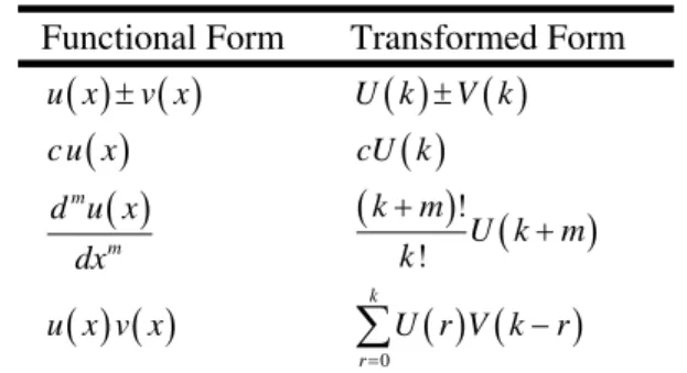
. (2.3)From above definitions it is easy to see that the concept of differential transform is derived from Taylor series expansion. With the aid of (2.1) and (2.2) the basic mathematical operations are readily be obtained and given in Table 1.
Table 1 One-dimensional differential transformation
Functional Form Transformed Form
u x v x U k
V k
c u x cU k
m
m
d u x dx
!!
k m
U k m
k
u x v x
0
k
r
U r V k r
B. Two Dimensional Differential Transform Method
Similarly, the two dimensional differential transform of the function w x t
, can be defined as follows:
(0,0) 1
, ,
! !
k h
k h
W k h w x t
k h x t
(2.4)
where w x t
, is the original function and W k h
, is the transformed function. The differential inverse transform of
,W k h is
,
, k hw x t W k h x t
. 2.5)Reduced Differential Transform Method for
Solving Klein Gordon Equations
Then combining equation (2.4) and (2.5) we write
0 0 (0,0)
1
, ,
! !
k h
k h k h
k h
w x t w x t x t
k h x t
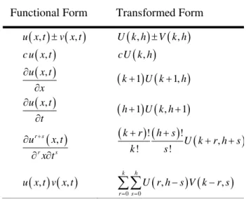
. (2.6)Therefore we can obtain basic mathematical operations of two-dimensional differential transform as follows in Table 2.
Table 2. Two dimensional differential transformation
Functional Form Transformed Form
, ,u x t v x t U k h
, V k h
,
,c u x t cU k h
,
,u x t x
k1
U k1,h
,u x t t
h1
U k h, 1
,r s
r s
u x t
x t
!
!
,
! !
k r h s
U k r h s
k s
, ,u x t v x t
0 0
, ,
k h
r s
U r h s V k r s
Now we can state our main results in the next section. III. REDUCED DIFFERENTIAL TRANSFORM FOR KLEIN–
GORDON EQUATIONS
The basic definitions and operations of reduced differential transform method [15-17] are introduced as follows:
Definition 1
If function u x t
, is analytic and differentiated continuously with respect to time t and space x in the domain of interest, then let
0 1
( ) ,
!
k
k k
t
U x u x t
k t
(3.1) where the t-dimensional spectrum function Uk
x is thetransformed function. In this paper, the lowercase u x t
, represent the original function while the uppercase
k
U x stand for the transformed function.
Definition 2
The reduced differential transform of a sequence
Uk x
k 0
is defined as follows:
0
, k k
k
u x t U x t
. (3.2) Then combining equation (3.1) and (3.2) we write
0 0
1
, ,
!
k
k k
k t
u x t u x t t
k t
. (3.3)Some basic properties of the reduced differential transformation obtained from definitions (3.1) and (3.2) are summarized in Table 3.
The proofs of Table 3 and the basic definitions of reduced differential transform method are available in [18].
To illustrate, Consider the following Klein–Gordon equations (1.1):
( , ) ( , ) ( , ) ( , ) ( , )
t x
L u x t L u x t u x t Nu x t f x t (3.4)
with initial conditions
( , 0) ( ), t( , 0) ( )
u x g x u x h x (3.5) where
2 2
2, 2
t x
L L
t x
, Nu x t( , ) is a nonlinear term.
Assume that we can write
, 0 0, n m
n m n m
u x t U t x
Then, we get terms
2 2 2 2
0,0, 0,1 , 0,2 ,..., 1,0 , 1,1 , 1,2 ,..., 2,0 , 2,1 ,...
U U x U x U t U tx U tx U t U t x
The first group can be written 0 0, 0
m m m
t U x
, the secondgroup as 1 1, 0
m m m
t U x
, the third group as 2 2, 0m m m
t U x
etc.Table 3. Basic operations of RDTM
Functional Form Transformed Form
( , )
u x t
0 1
, !
k
k
t
u x t
k t
, ,u x t v x t Uk( )x V xk( )
,u x t
Uk( )x ( is a constant)
m n
x t xm (k n)
( , )
m n
x t u x t ( )m
k n
x U x
, ,u x t v x t
0
( ) ( )
k
r k r
r
U x V x
( , )
r
r u x t
t
( )!
( ) ! k r
k r
U x
k
( , )
u x t x
Uk( )x
x
( , )
Nu x t
Maple code
NF:=Nu(x,t):#Nonlinear function odr:=3:# Order
u[t]:=sum(u[b]*t^b,b=0..odr): NF:=subs({Nu(x,t)=u[t]},NF): s:=expand(NF,t):
dt:=unapply(s,t): for i from 0 to odr do n[i]:=((D@@i)(dt)(0)/i!): print(N[i],n[i]); # Transform Function
Thus
0
, ( )n
n n
u x t U x t
where ,
0
( ) m
n n m
m
U x U x
so that the double series turns to a single series.Let the nonlinear term Nu x t( , ),write 1
0 0
( , ) ( ( ),..., ( )) n ( ) n
n n n
n n
Nu x t N U x U x t N x t
.Calculation of N xn( ) was given in the Table 3. The approximate solution using the t partial solution is given by:
1 1 1 1
( , ) t ( , ) t x ( , ) t ( , ) t ( , )
u x t L f x t L L u x t L Nu x t L u x t
(3.6) where
(0, ) t(0, ) ( ) ( )
u x tu x g x th x
and 1
0.
t t
t o
L
dtdt. Substituting for ( , ),u x t Nu x t( , ) we have0 0 0 0
2
2
0 0
0 0 0 0
0 0 0 ( ) ( ) ( ) ( ) ( ) ( ) ( ) t t n n n n n n
t t t t
n n n n n n t t n n n
U x t g x th x F x t dtdt
U x t dtdt N x t dtdt
x
U x t dtdt
We now carry out the above integrations to write 2
0 0
2 2 2
2
0 0
2
0
( ) ( ) ( ) ( )
( 1)( 2)
( ) ( )
( 1)( 2) ( 1)( 2)
( ) ( 1)( 2)
n n n n n n n n n n n n n n n t
U x t g x th x F x
n n
t t
U x N x
n n x n n
t U x n n
Let n n 2 on the right side. Then
2 0 2 2 2 2 2 2 2 2 2 ( ) ( ) ( ) ( ) ( 1) ( ) ( )
( 1) ( 1)
( ) ( 1) n n n n n n n n n n n n n n n t
U x t g x th x F x
n n
t t
U x N x
n n x n n
t U x n n
(3.7)Finally, equation coefficients of like powers of t, we derive the recursion formula for the coefficients (according to the RDTM and Table 3)
0( ) ( ), 1( ) ( )
U x g x U x h x (3.8)
and
2
2 2
( 2)!
( ) ( ) ( ) ( ) ( )
! n n n n n
n
U x F x U x N x U x
n x
(3.9) where Un( ),x F xn( ) and N xn( ) are the transformations of
the functions ( , ), ( , )u x t f x t and Nu x t( , ) respectively. Substituting (3.8) into (3.9) and by a straight forward iterative calculations, we get the following Un( )x values.
Then the inverse transformation of the set of values
( )
0p
n n
U x give approximation solution as,
0 ( , ) ( ) p n p n n
u x t U x t
where p is order of approximation solution.
Therefore, the exact solution of problem is given by ( , ) limp p( , )
u x t u x t
.
IV. APPLICATIONS
To show the efficiency of the new method described in the previous part, we present some examples.
A. Example 1
We first consider the homogeneous Klein–Gordon equation [11]
0
tt xx
u u u (4.1) with initial conditions:
( , 0) 1 sin( ), t( , 0) 0
u x x u x (4.2)
where uu x t
, is a function of the variables x and t. Then, by using the basic properties of the reduced differential transformation, we can find the transformed form of equation (4.1) as2
2 2
( 2)!
( ) ( ) ( )
! k k k
k
U x U x U x
k x
. (4.3)
Using the initial conditions (4.2), we have 0( ) 1 sin( ), 1( ) 0
U x x U x (4.4)
Now, substituting (4.4) into (4.3), we obtain the following Uk( )x values successively
2 3 4
5 6
1 1
( ) , ( ) 0, ( ) ,
2 24
1 ( ) 0, ( )
720
U x U x U x
U x U x
0, for k is odd ( ) 1
, for k is even ! k U x k
Finally the differential inverse transform of Uk( )x gives
0 0,2,4,...
1
, ( ) sin( )
!
k k
k
k k
u x t U x t x t
k
(4.5)Hence the closed form of (3.5) is
, sin( ) cosh( )u x t x t
which is the exact solutions of (4.1)–(4.2).
B. Example 2
We next consider the inhomogeneous nonlinear Klein-Gordon equation [21]
2 2 2
cos( ) cos ( )
tt xx
u u u x t x t (4.6) with the initial conditions:
( , 0) , t( , 0) 0
u x x u x (4.7)
Taking differential transform of (4.6) and the initial conditions (4.7) respectively, we obtain
2
2 2
( 2)!
( ) ( ) ( ) ( )
! k k k k
k
U x U x N x F x
k x
(4.8) where Nk
x and Fk
x are transformed form of
2 ,
For the easy to follow of the reader, we can give the first few nonlinear term are
2
0 0
1 0 1
2
2 0 2 1
3 0 3 1 2
( ) 2 ( ) ( )
2 ( ) ( ) ( ) 2 ( ) ( ) 2 ( ) ( )
N U x
N U x U x
N U x U x U x
N U x U x U x U x
2 0
1
2 2
3 0
2 0
F x x
F x
F x
F
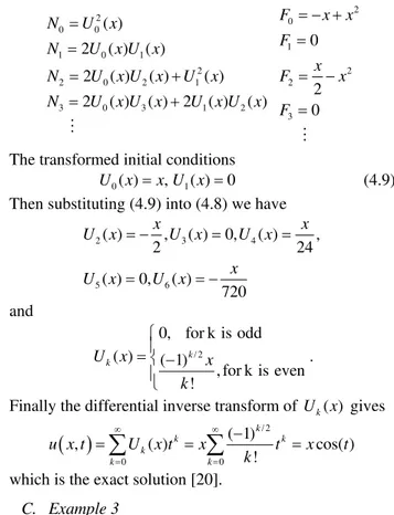
The transformed initial conditions
0( ) , 1( ) 0
U x x U x (4.9)
Then substituting (4.9) into (4.8) we have
2 3 4
5 6
( ) , ( ) 0, ( ) ,
2 24
( ) 0, ( ) 720
x x
U x U x U x
x
U x U x
and
/ 2
0, for k is odd ( ) ( 1)
, for k is even !
k k
U x x
k
.
Finally the differential inverse transform of Uk( )x gives
/ 20 0
( 1)
, ( ) cos( )
!
k
k k
k
k k
u x t U x t x t x t
k
which is the exact solution [20].
C. Example 3
We now consider the nonlinear Klein-Gordon equation [22]
3
3 3
0
4 2
tt xx
u u u u (4.10) with initial conditions
1
( , 0) sech( ), ( , 0) sech( )tanh( ) 2
t
u x x u x x x (4.11)
The exact solution of this problem is ( , ) sech
2
t
u x t x
. If we want to solve this equation by
means of RDTM, using Table 3, we can find the transformed form of equation (4.10) as
2
2 2
( 2)! 3
( ) ( ) ( ) ( )
! k k 4 k k
k
U x U x U x N x
k x
(4.12) where Nk
x is transformed form of 3 2
, 2u x t
and the
transformed initial conditions
0 1
1
( ) sech( ), ( ) sech( )tanh( ) 2
U x x U x x x (4.13)
Substituting (4.13) into (4.12), we obtain the following ( )
k
U x values successively.
Then, the inverse transformation of the set of values
60 ( )
k k
U x gives six-term approximation solution as Therefore, the exact solution of problem is given by
( , ) lim n( , )
n
u x y u x y
.
This solution is convergent to the exact solution [22] and the same as approximate solution of the variational iteration method [11]. (see Figure 1)
6 6
0
2 2
2 3
3 4
4 2
4 5
4 2
5 6
6
1 sinh( ) ( , ) ( )
cosh( ) 2 cosh( ) (cosh ( ) 2) (cosh ( ) 6) sinh( )
8 cosh ( ) 48cosh ( ) (cosh ( ) 20 cosh ( ) 24)
384 cosh ( )
(cosh ( ) 60 cosh ( ) 120) sinh( ) 3840 cosh ( )
(cosh ( )
k k k
x
u x t U x t t
x x
x x x
t t
x x
x x
t x
x x x
t x
x
4 2
6 7
182 cosh ( ) 840 cosh ( ) 720) 46080 cosh ( )
x x
t x
(4.14)
Figure 1. The comparison of the RDTM approximation
and the exact solution.
Figure 1 shows the comparison of the RDTM approximation solution of order six and the exact solution
( , ) sech 2
t
u x t x
, the solid line represents the solution
by the reduced differential transform method, while the circle represents the exact solution. From the figure 1, it is clearly seen that the RDTM approximation and the exact solution are in good agreement.
V. CONCLUSIONS
ACKNOWLEDGMENT
This study was supported by the Coordinatorship of Selcuk University’s Scientific Research Projects (BAP).
REFERENCES
[1] L. Debtnath, “Nonlinear Partial Differential Equations for Scientist and Engineers”, Birkhauser, Boston, 1997
[2] P.G. Drazin, R.S. Johnson, Solitons: An Introduction”, Cambridge University Press, Cambridge, 1983.
[3] M.J. Ablowitz, P.A. Clarkson, “Solitons, Nonlinear Evolution Equations and Inverse Scattering Transform, Cambridge University Press, Cambridge, 1990.
[4] A.M. Wazwaz, “Partial differential equations: methods and applications” The Netherlands: Balkema Publishers, 2002. [5] Santanu Saha Ray, “An application of the modified
decomposition method for the solution of the coupled Klein– Gordon–Schrödinger equation”, Communications in Nonlinear Science and Numerical Simulation, 13(7) 2008, 1311-1317.
[6] S.M. El-Sayed, “The decomposition method for studying the Klein-Gordon equation”, Chaos, Solitons & Fractals 18 (2003) 1025–1030.
[7] K. C. Basak, P. C. Ray, R. K. Bera, “Solution of non-linear Klein–Gordon equation with a quadratic non-linear term by Adomian decomposition method”, Communications in Nonlinear Science and Numerical Simulation, 14(3) 2009, 718-723.
[8] A. Ebaid, “Exact solutions for the generalized Klein–Gordon equation via a transformation and Exp-function method and comparison with Adomian’s method”, Journal of Computational and Applied Mathematics, 223(1) 2009,278-290.
[9] Z. Odibat, S. Momani, “A reliable treatment of homotopy perturbation method for Klein–Gordon equations”, Physics Letters A, 365(5-6) 2007, 351-357.
[10]Q. Sun, “Solving the Klein–Gordon equation by means of the homotopy analysis method”, Applied Mathematics and Computation,169 (1) 2005, 355-365.
[11]E. Yusufoglu, “The variational iteration method for studying the Klein–Gordon equation”, Applied Mathematics Letters, 21 (7) 2008, 669-674.
[12]N. Bildik, A. Konuralp, “The use of variational iteration method, differential transform method and Adomian decomposition method for solving different types of nonlinear partial differential equations”, International Journal of Nonlinear Sciences and Numerical Simulation 7 (1) (2006) 65–70.
[13]Q. Wang, D. Cheng, “Numerical solution of damped nonlinear Klein–Gordon equations using variational method and finite element approach”, Applied Mathematics and Computation, 162(1) 2005,381-401.
[14] J. Biazar, H. Ghazvini, “He’s variational iteration method for solving hyperbolic differential equations”, International Journal of Nonlinear Sciences and Numerical Simulation 8 (3) (2007) 311–314.
[15]Y. Keskin, G. Oturanc, “Reduced Differential Transform Method for Partial Differential Equations”, International Journal of Nonlinear Sciences and Numerical Simulation, 10 (6) (2009) 741-749.
[16]Y. Keskin, G. Oturanc, “Reduced differential transform method for solving linear and nonlinear wave equations”, Iranian Journal of Science & Technology, Transaction A, Vol. 34(A2) 2010, 113-122.
[17]Y. Keskin, G. Oturanc, “Reduced Differential Transform Method for fractional partial differential equations”, Nonlinear Science Letters A 1(2) (2010) 61-72.
[18]Y. Keskin, Ph.D. Thesis, Selcuk University (to appear). [19]A.S.V. Ravi Kanth, K. Aruna, “Differential transform method
for solving the linear and nonlinear Klein–Gordon equation”, Computer Physics Communications, 180(5) 2009, 708-711. [20]Saeid Abbasbandy, “Numerical solution ofnon-linear Klein–
Gordon equations by variational iteration method”, International Journal for Numerical Methods in Engineering, 70(7) 2006, 876-881.
[21]Wazwaz A. “The modified decomposition method for analytic treatment of differential equations”. Applied Mathematics and Computation 2006; 173:165–176.