Braz. J. Phys. vol.37 número4

(1)

Electrically Charged Pulsars

M. D. Alloy and D. P. Menezes

Depto de F´ısica - CFM - Universidade Federal de Santa Catarina Florian´opolis - SC - CP. 476 - CEP 88.040 - 900 - Brazil

Received on 27 April, 2007. Revised version received on 11 September, 2007

In the present work we investigate one possible variation on the usual electrically neutral pulsars: the inclusion of electric charge through a naive prescription. We study the effect of electric charge in pulsars assuming that the charge distribution is proportional to the energy density. All calculations were performed for equations of state obtained at zero temperature and also for fixed entropies. We then choose one of the models, the Nambu-Jona-Lasinio model for zero temperature quark stars without the inclusion of leptons, what makes them electrically charged, and compare the results with the previous one.

Keywords: Hadronic stars; Quark stars; Hybrid stars

I. INTRODUCTION

Pulsars are believed to be the remnants of supernova explo-sions. They have masses 1–2M_⊙, radii∼10 km, and a temper-ature of the order of 1011K at birth, cooling within a few days to about 1010K by emitting neutrinos. Pulsars are normally known as neutron stars, name that does not reflect their real composition, which is still a source of speculation. Some of the possibilities are the presence of hyperons [1–3], a mixed phase of hyperons and quarks [4–8], a phase of deconfined quarks or pion and kaon condensates [9]. Another possibility would be that pulsars are, in fact, quark stars [10]. In conven-tional models, hadrons are assumed to be the true ground state of the strong interaction. However, it has been argued [11–15] thatstrange mattercomposed of deconfinedu,dandsquarks could be the true ground state of all matter. In the stellar mod-eling, the structure of the star depends on the assumed EoS, which is different in each of the above mentioned cases. While neutron stars are bound by the gravitational force, quark stars are self-bound by the strong interaction.

Once an adequate EoS is chosen, it is used as input to the Tolman-Oppenheimer-Volkoff (TOV) equations [16], which are derived from Einstein’s equations in the Schwarzschild metric for a static, spherical star. Some of the stellar prop-erties, as the radius, gravitational and baryonic masses, cen-tral energy densities, etc are obtained. These results are then tested against some of the constraints provided by as-tronomers and astrophysicists [17, 18] and some of the EoS are shown to be inappropriate for describing pulsars [5, 6, 9].

One should also bear in mind that the temperature in the interior of the star is not constant [8, 19], but the entropy per baryon is. This is the reason for choosing fixed entropies to take the temperature effects into account. The maximum en-tropy per baryon (S) reached in the core of a new born star is about 2 (in units of Boltzmann’s constant) [20]. We then use EoS obtained withS=0(T =0), 1 and 2.

In the present work we investigate the effects of the elec-tric charge in compact stars. This study was first performed in stars composed of hot ionized gas [21] and then reconsidered for a cold star (T =0) described by a polytropic EoS [22]. The bulk of the stellar matter is expected to be electrically neutral. Only in the thin surface layer of several fermi there

is a non-vanishing electric field. It is commonly believed that the electric field in the bulk required to affect the EoS (of the order of 1020V/m) is well above the Schwinger field. Hence, thead hocassumption that the electric charge distribution is proportional to the mass density has mainly academic value. The TOV equations have to be modified to take the electric field into account. Then, in order to check how far away from the values obtained within a formalism that does not require charge neutrality, we have recalculated quark star properties from a model without leptons and consequentely, not charge neutral by construction. In this case the distribution of the electric charge is not uniform. We study the three possible kinds of pulsars: hadronic, hybrid and quarkionic with re-alistic EoS but the consideration of charged stars from first principles is only developed for quark stars built within the Nambu-Jona-Lasinio [23] model at zero temperature. Based on the general trend of the stellar matter properties we believe that the conclusions are general. Another possibility would be to include the eletromagnetic field in the Lagrangian density but in this case, a simple mean field approach would not be enough since it forces the eletromagnetic field to vanish and more sofisticated methods would be required.

This paper is organized as follows: in Sec. II the for-malisms of the electrically charged stars are revisited and the NJL model is discussed in some detail. In Sec. III the results are presented, discussed and the main conclusions are drawn.

II. FORMALISM AND RESULTS

As the first step we need to know the EoS of the system,

ε=ε(p), n=n(p),

(2)

32.5 MeV, the compression modulus is 300 MeV and the ef-fective mass is 0.7M. For the meson-hyperon coupling con-stants we have chosen them constrained by the binding of the Λhyperon in nuclear matter, hypernuclear levels and neutron star masses (xσ=0.7 andxω=xρ=0.783) and have assumed that the couplings to theΣ andΞ are equal to those of the Λhyperon [26, 27]. For the construction of the EoS for hy-brid stars, the hadronic phase was obtained with the non-linear Walecka model and the parameters above and the quark phase with the MIT bag model withBag= (180 MeV)4_{. For the} quark stars within the MIT model [25], we have usedmu= md=5.5 MeV,ms=150.0 MeV andBag= (180 MeV)4. For the purpose of the present work, the value of the bag parame-ter does not play an important role. Concerning quark stars within the NJL model [23], the set of parameters were chosen in order to fit the values in vacuum for the pion mass, the pion decay constant, the kaon mass and the quark condensates as in [28, 29].

A. Electrically charged compact stars

In this section we include modifications in the TOV equa-tions to describe electrically charged pulsars with null angular velocity. The geometry that describes a static spherical star is given by equation (1). In order that the Maxwell equations are incorporated into the stress tensorTνµ, it becomes:

T_νµ= (p+ε)uµuν−pδµν+ 1 4π

µ

FµαFαν−1 4δ

µ νFαβFαβ

¶

, (1)

where again pis the pressure,εis the energy density, anduµ is the 4-velocity vector.

The electromagnetic field obeys the relation £√

−gFµν¤

,ν=4πj

µ√₋_g_, ₍₂₎

where jµis the four current density. Next we consider static stars only. Hence the electromagnetic field is only due to the electric charge, which means thatF01₌₋_F10_{, and the other} terms are absent. From the four-potential Aµ the surviving potential isA0=φ. Thus the electric field is given by

E(r) = 1

r2 Z r

0 4π

r2j0e(ν+λ)/2dr, (3) wherej0eν/2=ρchis the charge density. The electric field can be written as

dE(r)

dr =− 2E

r +4πρche λ/2

(4)

and total charge of the system as

Q=

Z R 0

4πr2ρcheλ/2dr, (5) whereRis the radius of the star.

In the star frame the mass is dMtot

dr (r) =4πr 2

µ

ε+E(r) 2

8π ¶

. (6)

To an observer at infinity, the mass is

M∞= Z ∞

0 4π r2

µ

ε+E(r) 2

8π ¶

dr=Mtot(R) + Q(R)2

2R . (7) By using the conservation law of the stress tensor(Tν;µµ =0) we obtain the hydrostatic equation

d p dr = −

h

Mtot+4πr3 ³

p₋E_8π(r)2´i(ε+p)

r2³₁₋2Mtot

r ´

+ ρchE(r)eλ/2. (8)

The first term on the right-hand side comes from the gravi-tational force and the second term comes from the Coulomb force. By using the metric and the relation

Rµν−1 2Rδ

µ

ν=−8πTνµ, (9) we obtain the following differential equation

dλ

dr = "

8πreλ µ

ε+E(r) 2

8π ¶

−

Ã eλ₋1

r !#

, (10)

which is used to determine the metriceλ.

So, we have a set of differential equations to be solved formed by equations(19), (21), (23) and (25). The boundary conditions atr=0 areE(r) =0,eλ=1,n=ρcand atr=R, p=0. We assume that the charge goes with the energy density εas prescribed in [22]:

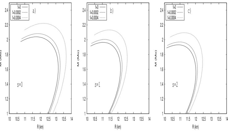
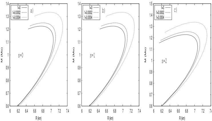
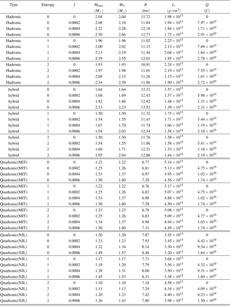
ρch=f×0.86924×103ε. (11) According to [22], this choice of charge distribution is a rea-sonable assumption in the sense that a large mass can hold a large amount of charge. One should bear in mind, however, that the EoS used in the present work were built electrically neutral and then f has to be a very small quantity. In table I results for electrically charged neutron stars are presented. We have calculated the results for 48 different configuration mod-els of compact stars. The EoS for hadronic and hybrid stars were taken from [8], the EoS for quark stars were taken from [10]. In table I the electric chargeQis given in Coulomb and f varies from zero (no charge) to a small value (0.0006). The related mass-radius plots for hadronic, hybrid and quark stars are given respectively in Figs. 4, 5 and 6-7. For quark stars we present two sets of calculations, one for EoS obtained with the MIT bag model and another one for EoS obtained with the Nambu-Jona-Lasinio model because their strangeness compo-sitions are very different, as seen in [10].

(3)

NJL

NJL*

−4

p (fm )

ρ/ρ0 −0.5

0 0.5 1 1.5 2 2.5

0 2 4 6 8 10 12 14

FIG. 1: EoS obtained forS=0 within the NJL model.

NJL* NJL

ρ/ρ₀

Ys

0 0.05 0.1 0.15 0.2 0.25 0.3

2 4 6 8 10 12 14

FIG. 2: Strangeness content obtained forS=0 within the NJL model.

B. The NJL model and charge neutrality

The main aspects of the construction of equation of states with one of the models used in the present work, the Nambu-Jona-Lasinio (NJL) model [28, 30, 31], that includes most of the symmetries of QCD, including chiral symmetry are dis-cussed as follows. For the other models, please refer to [8, 10] among many other papers in the literature.

The NJL model is defined by the Lagrangian density

LNJL = q¯(iγµ∂µ−m)q + gS

8

∑

a=0

[ (q¯λa_q₎2 _{+ (} ¯

q iγ5λaq)2] (12) + gD{det[q¯i(1+γ5)qj] +det[q¯i(1−γ5)qj]}, whereq= (u,d,s)are the quark fields andλa(0 ≤a ≤8) are the U(3) flavor matrices. The model parameters are:m= diag(mu,md,ms), the current quark mass matrix (md=mu), the coupling constants gS and gD and the cut-off in three-momentum space,Λ. The NJL model is valid only for quark momenta smaller than the cut-offΛ.

The baryonic thermodynamical potential density is given by

ΩB=−PB=

E

B−T

S

B−

∑

i

µiρi−Ω0, (13) µ

ρ/ρ0

µ µ * µn

e n

0 200 400 600 800 1000 1200 1400 1600

2 4 6 8 10 12 14

FIG. 3: Neutron and electron chemical potentials forS=0 within

the NJL model.

where the energy density is

E

_B₌ ₋ ₂Nc

∑

i

Z _d3_p

(2π)3

p2+miMi

Ei ×

[(ni−−ni+)θ(Λ2−p2)]

− 2gS

∑

i=u,d,s

hq¯iqii2−2gDhuu¯ ihdd¯ ihss¯i

−

E

₀ ₍₁₄₎

and the entropy density is

S

_B₌ ₋ ₂Nc

∑

i=u,d,s Z _d3_p

(2π)3θ(Λ

2₋_p2₎_× [[ni+ln(ni+) + (1−ni+)×

ln(1−ni+)] + [ni+→ni−]]. (15) In the above expressionsNc=3,T is the temperature,µi(ρi) is the chemical potential (density) of particles of typeiand

E

₀

andΩ0are included in order to ensure

E

=Ω=0 in the vac-uum. This requirement fixes the density independent part of the EoS.n(_i∓)are the Fermi distribution functions of the neg-ative (positive) energy states. Minimizing the thermodynam-ical potentialΩwith respect to the constituent quark masses Mileads to three gap equations for the massesMi

Mi =mi−4gShq¯iqii −2gDhq¯jqjihq¯kqki, (16) with cyclic permutations ofi, j,k.

In a star with quark matter both beta equilibrium and charge neutrality [26] are normally required. Forβ-equilibrium mat-ter we must add the contribution of the leptons as free Fermi gases (electrons and muons) to the energy density, pressure and entropy density. The relations between the chemical po-tentials of the different particles are then given by

µs=µd=µu+µe, µe=µµ. (17) For charge neutrality we must impose

ρe+ρµ= 1

(4)

1

1.2

1.4

1.6

1.8

2

2.2

2.4 10 10.5 11 11.5 12 12.5 13 13.5 14

M (Mo)

R (km)

s=0

a)

f=0

f=0.0002

f=0.0004

1

1.2

1.4

1.6

1.8

2

2.2

2.4 10 10.5 11 11.5 12 12.5 13 13.5 14

M (Mo)

R (km)

s=1

b)

f=0

f=0.0002

f=0.0004

1

1.2

1.4

1.6

1.8

2

2.2

2.4 10 10.5 11 11.5 12 12.5 13 13.5 14

M (Mo)

R (km)

s=2

c)

f=0

f=0.0002

f=0.0004

FIG. 4: Solutions for electrically charged hadronic stars with different values off.

0.4

0.6

0.8

1

1.2

1.4

1.6

1.8

2 10 10.5 11 11.5 12 12.5 13 13.5 14

M (Mo)

R (km)

s=0

a)

f=0

f=0.0002

f=0.0004

0.4

0.6

0.8

1

1.2

1.4

1.6

1.8

2 10 10.5 11 11.5 12 12.5 13 13.5 14

M (Mo)

R (km)

s=1

b)

f=0

f=0.0002

f=0.0004

0.4

0.6

0.8

1

1.2

1.4

1.6

1.8

2 10 10.5 11 11.5 12 12.5 13 13.5 14

M (Mo)

R (km)

s=2

c)

f=0

f=0.0002

f=0.0004

(5)

0.6

0.7

0.8

0.9

1

1.1

1.2

1.3

1.4

6

6.2

6.4

6.6

6.8

7

7.2

7.4

M (Mo)

R (km)

s=0

a)

f=0

f=0.0002

f=0.0004

0.6

0.7

0.8

0.9

1

1.1

1.2

1.3

1.4

6

6.2

6.4

6.6

6.8

7

7.2

7.4

M (Mo)

R (km)

s=1

b)

f=0

f=0.0002

f=0.0004

0.6

0.7

0.8

0.9

1

1.1

1.2

1.3

1.4

1.5

6

6.2

6.4

6.6

6.8

7

7.2

7.4

M (Mo)

R (km)

s=2

c)

f=0

f=0.0002

f=0.0004

FIG. 6: Solutions for electrically charged quark stars obtained with the MIT bag model for different values of f.

0.4

0.5

0.6

0.7

0.8

0.9

1

1.1

1.2

1.3

1.4

6

6.5

7

7.5

8

8.5

9

M (Mo)

R (km)

s=0

a)

f=0

f=0.0002

f=0.0004

0.4

0.5

0.6

0.7

0.8

0.9

1

1.1

1.2

1.3

1.4

6

6.5

7

7.5

8

8.5

9

M (Mo)

R (km)

s=1

b)

f=0

f=0.0002

f=0.0004

0.4

0.5

0.6

0.7

0.8

0.9

1

1.1

1.2

1.3

1.4

6

6.5

7

7.5

8

8.5

9

M (Mo)

R (km)

s=2

c)

f=0

f=0.0002

f=0.0004

(6)

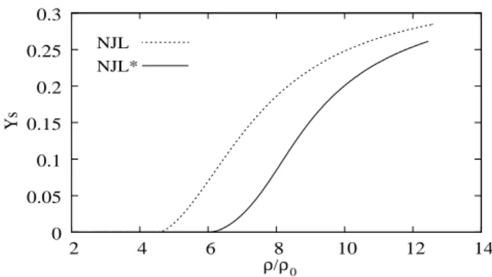
In the present work we have also desconsidered the usual hypothesis of charge neutrality and beta equilibrium by not adding any leptons and, in this case, the system becomes nat-urally charged. We refer to the charged EoS as NJL*. In Fig. 1 both EoS are displyed. The main effects appear at interme-diate energy densities.

In Figs. 2 and 3ρis the total baryonic density andρ0is its value at the nuclear matter saturation point. We investigate the strangeness content (Ys=ρs/ρ) of both EoS in Fig. 2, from where we can see that strange quarks appear at much higher densities in a charged star. This is due to the fact that it has a mass much larger than theuanddquarks and since no charge neutrality orβ-equilibrium are imposed, it does not have to artificially appear to compensate for the electric charge and/or the electron chemical potential. The chemical potentials of both models are shown in Fig. 3. In the usual NJL model the quark chemical potentials are defined asµq=µn/3−eqµe, whereµnis the neutron chemical potential and eq the elec-tric charge of each quark. The electron chemical potential is only present in the charge neutral EoS. Hence, in the NJL*, as no electrons are introduced, all quark chemical potentials are identical, as seen also from eq.(17), but the Fermi momenta remain different because they depend on the quark masses as well. Information on the net electric charge can be read off Figs. 2 and 3.

III. RESULTS AND CONCLUSIONS

Let’s now go back to the stellar matter properties in order to compare them with what is found in the literature and draw the conclusions. In Table I we show, for each EoS investigated and different values of f, the maximum stellar mass, the mass at infinity, the radius, the central energy density and the elec-tric charge the star can hold. Notice thatMmax stands for the maximum value of a family of stars in each of the curves dis-played whileMtot refers to the mass when the electric charge is included in anad hoc way, as seen in eq.(6). All the cor-responding curves for the mass versus radius are plotted in Figs. 4-7. The general trend is the same observed in a sim-ple polytropic EoS for T =0 [22], i.e., the electric charge, the maximum mass and the mass observed at infinity increase with f, as it should be. Although the EoS used in the present work are very different from the one used in [22] the values of the radii obtained and the electric charge for a fixed f value are compatible. Figs. 4, 5, 6 and 7 also show the same be-havior as fig. 2 of [22], i.e., as f increases, the maximum mass and radius of a family of stars increase. The EoS used in the present work are for bare pulsars, i.e. the crust is not in-cluded. From table I one can see that the effect of entropy on a charged star remains the same as in a neutral star: the max-imum masses and the radii decrease with the increase of the entropy for hadronic and quark stars within the NJL model. For hybrid and MIT stars the behavior is not so well defined.

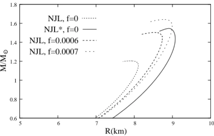
We now turn to the comparison of the quark star properties obtained both with the neutral NJL model with electric charge includedby hand and its charged version. The mass radius graph is shown in Fig. 8 forS=0. One can see that the max-imum mass of the naturally charged star appears in between stars with f =0.006 and f =0.007, a quite high factor that corresponds to a reasonably large electric charge. The radius of the naturally charged star is a bit larger than their coun-terparts but the values are within the expected range. This study has shown that thead hocassumption that the charge is distributed in a rate proportional to its energy density does, af-ter all, contain some correct physics. The conclusions drawn for the NJL model are general and are also valid for naturally charged hadronic and hybrid stars. It is worth emphasizing that we do believe that the presence of leptons are mandatory, at least in the outmost layer of the star since electron-positron pairs do escape from pulsars and are detected by astronomers.

NJL, f=0.0006 NJL, f=0.0007 NJL, f=0 NJL*, f=0

R(km) .

M/M

0.6 0.8 1 1.2 1.4 1.6 1.8

5 6 7 8 9 10

FIG. 8: Solutions for electrically charged quark stars obtained with

the NJL model for different values of f and the corresponding

charged version.

In the present work we have investigated one possible vari-ation on the usual electrically neutral pulsars: the electric charge is included in an ad hoc way. We have observed that the behaviors shown in previous works with much sim-pler EoS were also observed here. The influence of the tem-perature was also investigated by means of fixed entropy per baryon. The charge effect does not alter previous conclusions related to the mass and radius behavior of protoneutron stars with larger entropy [8, 10].

Acknowledgments

This work was partially supported by CNPq (Brazil). M.D.A. would like to thank CNPq for a master degree schol-arship. We thank an anonymous referee for suggestions that helped the improvement of this work.

[1] A.L. Esp´ındola and D.P. Menezes, Phys. Rev. CC65, 045803

(2002).

(7)

(2004).

[3] R. Cavangnoli and D.P. Menezes, Braz. J. Phys. B 35, 869

(2005).

[4] D.P. Menezes and C. Providˆencia, Phys. Rev. C68, 035804

(2003).

[5] D.P. Menezes and C. Providˆencia, Phys. Rev. C 70, 058801

(2004); D.P. Menezes and C. Providˆencia, Braz. J. Phys. 34,

724 (2004).

[6] P.K. Panda, D.P. Menezes, and C. Providˆencia, Phys. Rev. C69,

025207 (2004).

[7] P.K. Panda, D.P. Menezes, and C. Providˆencia, Phys. Rev. C69,

058801 (2004).

[8] D.P. Menezes and C. Providˆencia, Phys. Rev. C 69, 045801

(2004).

[9] D.P. Menezes, P.K. Panda, and C. Providˆencia, Phys. Rev. C72

, 035802 (2005).

[10] D.P. Menezes and D.B. Melrose, Publ. Astron. Soc. Aust.22,

292 (2005); D.P. Menezes, C. Providˆencia, and D.B. Melrose,

J. Phys. G: Nucl. Part. Phys.32, 1081 (2006).

[11] N. Itoh, Prog. Theor. Phys.291, 44 (1970).

[12] A.R. Bodmer, Phys. Rev. D4, 1601 (1971).

[13] E. Witten, Phys. Rev. D30, 272 (1984).

[14] P. Haensel, J.L. Zdunik, and R. Schaeffer, Astron and

Astro-phys.160, 121 (1986).

[15] C. Alcock, E. Farhi, and A. Olinto, Astrophys. J. 310, 261

(1986).

[16] R.C. Tolman, Phys. Rev.55, 364 (1939); J.R. Oppenheimer and

G.M. Volkoff, Phys. Rev.55, 374 (1939).

[17] J. Cottam, F. Paerels, and M. Mendez, Nature420, 51 (2002).

[18] D. Sanwal, G.G. Pavlov, V.E. Zavlin, and M.A. Teter,

Astro-phys. J574, L 61 (2002).

[19] A. Burrows and J. M. Lattimer, Astrophys. J.307, 178 (1986).

[20] M. Prakash, I. Bombaci, M. Prakash, P. J. Ellis, J. M. Lattimer,

and R. Knorren, Phys. Rep.280, 1 (1997).

[21] S. Rosseland, Mon. Not. R. Astron. Soc.84, 720 (1924).

[22] A.L. Esp´ındola, M. Malheiro, J.P.S. Lemos, and V.T. Zanchin,

Phys. Rev. C68, 084004 (2005).

[23] Y. Nambu and G. Jona-Lasinio, Phys. Rev.122, 345 (1961);

124, 246 (1961).

[24] B. Serot and J.D. Walecka,Advances in Nuclear Physics16,

Plenum-Press, (1986) 1.

[25] A. Chodos, R.L. Jaffe, K. Johnson, C.B. Thorne, and V.F.

Weis-skopf, Phys. Rev. D9, 3471 (1974).

[26] N. K. Glendenning, Compact Stars, (Springer-Verlag,

New-York, 2000).

[27] N. K. Glendenning and S.A. Moszkowski, Phys. Rev. Lett.67,

2414 (1991).

[28] C. Ruivo, C. Sousa, and C. Providˆencia, Nucl. Phys. A651, 59

(1999).

[29] T. Kunihiro, Phys. Lett. B219, 363 (1989).

(8)

TABLE I: Electrically compact stars with different charge fractionf.

Type Entropy f Mmax M∞ R εc Q

(M_⊙) (M_⊙) (km) (g/cm3) (C)

Hadronic 0 0 2.04 2.04 11.72 1.98×1015 0

Hadronic 0 0.0002 2.08 2.10 11.84 1.94_×1015 ₇_.₉₇_×₁₀19

Hadronic 0 0.0004 2.22 2.28 12.18 1.84×1015 1.71×1020

Hadronic 0 0.0006 2.50 2.66 12.73 1.75×1015 2.91×1020

Hadronic 1 0 1.96 1.96 11.02 2.23×1015 0

Hadronic 1 0.0002 2.00 2.02 11.15 2.13×1015 7.69×1019

Hadronic 1 0.0004 2.13 2.19 11.44 2.04×1015 1.64×1020

Hadronic 1 0.0006 2.39 2.55 12.01 1.85_×1015 ₂_.₇₈_×₁₀20

Hadronic 2 0 1.93 1.93 10.91 2.24×1015 0

Hadronic 2 0.0002 1.97 1.98 11.01 2.19×1015 7.55×1019

Hadronic 2 0.0004 2.09 2.15 11.26 2.15×1015 1.61×1020

Hadronic 2 0.0006 2.34 2.50 11.86 1.90_×1015 ₂_.₇₂_×₁₀20

hybrid 0 0 1.64 1.64 12.33 1.57×1015 0

hybrid 0 0.0002 1.68 1.69 12.43 1.57×1015 5.98×1019

hybrid 0 0.0004 1.82 1.86 12.82 1.48×1015 1.31×1020

hybrid 0 0.0006 2.13 2.23 13.52 1.39×1015 2.31×1020

hybrid 1 0 1.50 1.50 11.32 1.75_×1015 ₀

hybrid 1 0.0002 1.54 1.55 11.43 1.71×1015 5.44×1019

hybrid 1 0.0004 1.67 1.70 11.74 1.66×1015 1.19×1020

hybrid 1 0.0006 1.94 2.03 12.34 1.58×1014 2.10×1020

hybrid 2 0 1.50 1.50 11.76 1.58_×1015 ₀

hybrid 2 0.0002 1.54 1.55 11.86 1.58×1015 5.41×1019

hybrid 2 0.0004 1.68 1.71 12.21 1.53_×1015 ₁_.₁₈_×₁₀20

hybrid 2 0.0006 1.95 2.04 12.86 1.44×1014 2.10×1020

Quarkonic(MIT) 0 0 1.22 1.22 6.77 5.14×1015 0

Quarkonic(MIT) 0 0.0002 1.25 1.26 6.81 5.13×1015 4.75×1019

Quarkonic(MIT) 0 0.0004 1.33 1.37 6.97 4.95_×1015 ₁_.₀₂_×₁₀20

Quarkonic(MIT) 0 0.0006 1.50 1.60 7.28 4.56×1015 1.74×1020

Quarkonic(MIT) 1 0 1.22 1.22 6.76 5.17×1015 0

Quarkonic(MIT) 1 0.0002 1.25 1.26 6.82 5.07×1015 4.75×1019

Quarkonic(MIT) 1 0.0004 1.33 1.37 6.98 4.88×1015 1.02×1020

Quarkonic(MIT) 1 0.0006 1.50 1.60 7.29 4.50×1015 1.74×1020

Quarkonic(MIT) 2 0 1.23 1.23 6.79 5.08×1015 0

Quarkonic(MIT) 2 0.0002 1.25 1.26 6.83 5.09×1015 4.77×1019

Quarkonic(MIT) 2 0.0004 1.34 1.37 6.98 4.94×1015 1.03×1020

Quarkonic(MIT) 2 0.0006 1.50 1.60 7.31 4.49×1015 1.74×1020

Quarkonic(NJL) 0 0 1.20 1.20 7.87 3.45×1015 0

Quarkonic(NJL) 0 0.0002 1.23 1.23 7.93 3.45×1015 4.42×1019

Quarkonic(NJL) 0 0.0004 1.32 1.34 8.14 3.30×1015 9.54×1019

Quarkonic(NJL) 0 0.0006 1.49 1.57 8.48 3.20×1015 1.64×1020

Quarkonic(NJL) 1 0 1.17 1.17 7.71 3.68×1015 0

Quarkonic(NJL) 1 0.0002 1.19 1.20 7.79 3.56_×1015 ₄_.₃₂_×₁₀19

Quarkonic(NJL) 1 0.0004 1.28 1.31 8.00 3.50×1015 9.31×1019

Quarkonic(NJL) 1 0.0006 1.45 1.53 8.31 3.38×1015 1.60×1020

Quarkonic(NJL) 2 0 1.10 1.10 7.18 4.58×1015 0

Quarkonic(NJL) 2 0.0002 1.13 1.13 7.29 4.34×1015 4.09×1019

Quarkonic(NJL) 2 0.0004 1.20 1.23 7.42 4.40×1015 8.23×1019