Abstract
— The induction planar actuator, i.e. IPA, proposed in this
study presents an electromagnetic structure formed by a static
ferromagnetic core with an aluminium plate that corresponds to
the secondary, and a mover, also called primary. The latter
comprehends two three-phase windings, mounted in an armature
core, which are orthogonal to each other. When they are fed by
three-phase AC excitations, a moving magnetic field takes place,
and can travel along the
x
-axis and the
y
-axis direction
simultaneously. The travelling magnetic field induces electrical
currents in the secondary. The interaction between the moving
magnetic field from the primary and the magnetic field originated
by the induced current in the secondary produces a planar force.
That explains the primary movement over the working area
defined by the secondary. The 3D flux density distribution of the
actuator suggests the employment of a grain-insulated soft
magnetic composite to reduce eddy currents and losses on the core
of the primary armature core. Magnetic flux density, induced
current and planar traction forces are studied.
Index Terms— Induced current, magnetic flux density, planar actuator, planar movement, planar traction force, soft magnetic composite material.
I.
INTRODUCTIONPlanar drivers play an important role in several industrial areas, e.g. semiconductor manufacturing system, inspection of surfaces, machines tools engineering, precision planar movements and others [1, 2, 3, 4]. The special requirements to planar drives concerning structural and functional parameters depend on their application. According to the requirements, energy converter principles and types of construction are applied. Typically, it can be achieved by an assembly that employs two motors: one is responsible for handling the x -axis, and another, for the y-axis in a Cartesian coordinate system. The control is carried out by means of control methods combined with power electronics devices [4, 5, 6]. Most existing planar drives, mainly the permanent magnet ones, were developed for high positioning accuracy precision and fast dynamic applications.
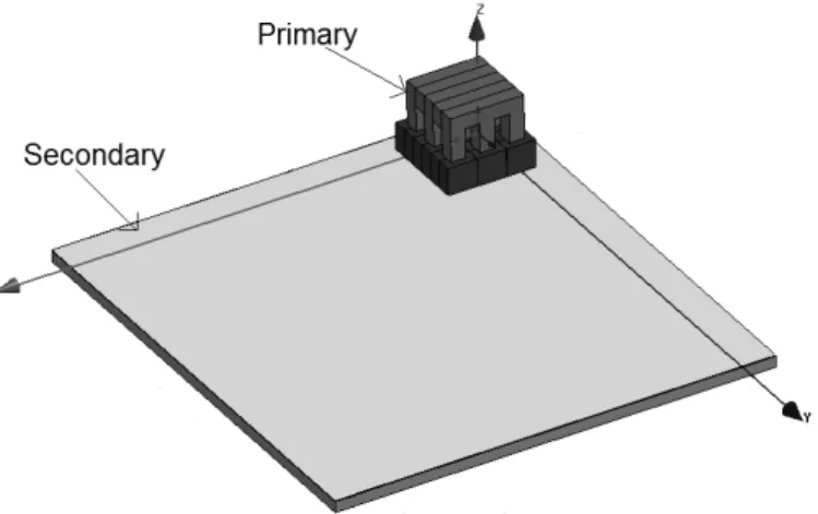
The induction planar actuator, as proposed in this work, can produce bi-directional motion based on a single traction device over a plane called the working area of the actuator. It relies on a mover, i.e. the primary, with two three-phase orthogonal armature coils and on a 3D distribution of magnetic flux density. Figure 1 shows the schematic of the IPA and its parts. The use of materials such as the high resistivity soft magnetic composite has enabled a proper design and the implementation of the IPA [6, 7, 8]. The actuator presents no cogging force. Its working plane is defined solely by the secondary dimensions, and that can have any larger size than the mover.
In this paper, the magnetic flux density in the air gap region will be investigated as a function of the primary excitation. Also, the induced current in the secondary materials as function of these excitations are a
An Analysis on Electric and Magnetic
Behaviour on an Induction Planar Actuator
Nolvi Francisco Baggio Filho and Aly Ferreira Flores Filho
Post Graduate Program in Electrical Engineering
topic of the research. Moreover, the behaviour of the planar traction force, due to the interaction between those two quantities, will be analysed as function of slip.
Fig. 1. Perspective view of the actuator and its parts [6].
II. PLANAR ACTUATOR TOPOLOGY AND DESIGN
The Induction Planar Actuator (IPA) is divided into two parts: moving part and static one. The moving primary part comprehends a core formed by a grain-insulated soft magnetic composite (SMC) block with nine teeth where eighteen coils are wound. The coils are divided in two sets of nine. The two sets of coils are placed in a way that they are orthogonal to each other: one set corresponds to the x-axis, and the other, to the y-axis. Each set of coil is fed by its own three-phase AC source [8, 9]. The static secondary consists of a slab of aluminium placed on the top of a slab of soft ferromagnetic material, e.g. massive steel. Figure 2 shows the frontal view. The main dimensions of the IPA are given in Table I.
TABLE I. SPECIFICATIONS AND DIMENSIONS OF THE INDUCTION PLANAR ACTUATOR
Symbol Quantity Value
2 length of the mover 100mm
h1 height of primary base 15mm
h2 height of the legs 40mm
h3 thickness of the aluminum 1mm
h4 thickness of the steel 6mm
h5 height of the coils 18mm
hg thickness of the air gap 0.5mm
d1 length between the legs 20mm
d2 length of the legs 20mm
d3 length of the coils 38mm
m number of phases per winding 3
p number of poles per winding 1
n number of coils per phase 3
N number of turns per coil 250
W number of windings 2(x and y)
Each tooth receives two primary coils electrically independent from each other: one form the set of three phase windings to produce a magnetic flux travelling in the x direction, the other will form the set of three phase windings to produce a magnetic flux travelling in the y direction. Each set of three phase windings has a star connection with no neutral, Figure 3. Each coil consists of 250 turns distributed in 11 layers, with an electrical resistance of approximately1.21Ω. In order to prevent a significant temperature rise, a 4 A/mm2 was adopted for the design of those coils.
This assembly of windings was chosen by practicality and maintenance. However, as the three windings x and y are in different layers or positions in relation to the air gap, the electromagnetic effects of each one of them will be different. The main reason for each phase of each winding to be composed by 3 coils is because in this configuration the magnetic flux has less leakage and is more concentrated on the preferred path through the air gap.
III. OPERATION PRINCIPLES
The operating principle of the induction planar actuator is based on the same principle of a linear induction motor.
The primary core topology combined with the three-phase excitation is responsible for producing the magnetomotive force and a magnetic field that can travel along a straight line in the x-direction and/or in the y -direction. As a result, the two directions of the travelling magnetic field are orthogonal to each other [6, 10, 11]. That results in an induced current in the secondary, mostly on the aluminium slab. The induced current and its interaction with the travelling magnetic fields are responsible for the production of the planar propulsion force that pushes the mover along a straight line. Hence, the direction of movement of the mover will depend on the phase sequences and on the magnetomotive force produced by each three-phase set of coils.
The use of a steel slab in the secondary would increase de air gap flux density, and, hence, the planar traction force. However, it will also result in an increased normal force parallel to z direction. The travelling magnetic field also causes magnetic losses in the ferromagnetic material [8].
The use of an SMC material, e.g. 1P Somaloy 500, in the primary, limits the losses produced by eddy currents. At the same time it allows a 3D flux density distribution by being isotropic. It has a higher electrical resistivity, but a lower magnetic permeability when compared to massive steel [6]. Nevertheless, it should not be a cause of major concern since a 1 mm long air gap is present and that will set the air gap flux density. Table II shows the characteristics of the two ferromagnetic materials employed in the case for the sake of the comparison.
TABLE II. THE FERROMAGNETIC MATERIAL EMPLOYED BY THE IPA [6]
Quantity AISI 1020 steel (stator back iron)
Somaloy 500 (armature core)
Maximum relative permeability 3800 500
Resistivity (µ m) 0.1862 70
Density (g/mm3) 7.85
7.53
IV. ANALYTICAL MODELING
The three-dimensional distribution of magnetic flux density in the air gap of the IPA is closely connected with the production of electromagnetic forces acting on the device. The behaviour of that flux density depends directly on the constructive features of the machine, and on how the primary excitation is produced.
(a) (b) (c)
Fig. 4. Region where the air-gap magnetic flux density is analysed: (a) frontal view;
(b) top view and; (c) instant of time considered.
A. Magnetic Field
It must be underlined that in the air gap of the IPA there are the effects of two sources of magnetic flux: the first one is a result of the travelling magnetic field produced by the primary excitation; the second one results from the eddy currents induced in the secondary. The effects of those magnetic fields are considered together in order to obtain a resulting magnetic field and the traction force.
The equation that allows one to model the distribution of magnetic flux density in the air gap when eddy currents are not considered is obtained by solving (1). Also, the equation used to model the influence of the field produced by those currents in the secondary is the solution of the differential equation as given by (2) [10].
0
2 2
2 2
2 2
=
∂
Ψ
∂
+
∂
Ψ
∂
+
∂
Ψ
∂
z
y
x
g g
g
(1)
k y A j z A
A x x
∂ ∂ − ∂ ∂ = ×
∇ (2)
g
Ψ
is the magnetic scalar potential in the air gap,A
is the magnetic vector potential associated with themagnetic flux density through B=∇×A [11, 12].
For the analytical modelling, the boundary conditions are defined in a way that the magnetic scalar potential was equal to zero on planes x=0, y=0, z=0, x=lt/2, y=lt/2, z=lg+la, x=lt, y=lt, z=lg+la. Figure 3 helps to understand
that.
According to [7] and [9], the effect of the alternating magnetic field that produces the resulting magnetic flux density in the air gap is possible to obtain as a function of time. Then, from the combination of sources of magnetic field, the resulting magnetic flux density in the air gap can be expressed by (3).
)
(
)
,
,
(
)
,
,
,
(
x
y
z
t
B
x
y
z
B
t
B
=
(3) B. Development of the Modelling Equation of the Magnetic Fieldthe equation comes as the solution from the Poisson’s equation in terms of magnetic scalar potential, considering the boundary conditions as set.
(
)
(
)
(
−)
− + = ∞ = + + − y l m x l n nm l ml l nl e e e e e A B t t t p t p m n l l l l l z z Dg b g
g b g π π γ π π π µ γ γ γ γ γ 2 sin 2 sin 1 2 cos 2 cos 1 8 ... 3 , 1 , ) ( 2 ( ) 2 ( ( ) ( ) ( ) ( 2 0 0 1
(4)
where 2 n2 m2
lt +
= π
γ . When both windings are excited, the magnetic flux density produced by the primary
excitation can be written as (5)
y g x g
g
B
B
B
1=
1+
1 (5)That formulation of
B
g1 refers to a static magnetic field and considers a source of magnetic potentialA
0 asif it were under a DC excitation.
A
0is given by (6) [9, 13, 14].(
g)
(
g)
[ ]
myAl A l z senh M l z M k M
A = 1 4cosh ( − ) − 3 ( − )
6
0 β β
β (6)
It is considered that
) ( )
cosh( 1
1 Fe Fe
Fe Fe Fe rFe h k senh k h k M
β
µ
+= (7)
) ( 1 ) cosh(
2 Fe Fe
rFe Fe Fe Fe h k senh h k k M µ β +
= (8)
) ( . ) cosh( 2 1
3 Al Al
Al Fe Al Al
rFe M senhk h
k k h k M
M =µ + (9)
) ( )
cosh( 1
2
4 Al Al rFe Al Al
Al
Fe M k h M senh k h
k k
M = +
µ
(10)) ( ) cosh( 4 3 5 g Al
g M senh l
k l M M β β β +
= (11)
) ( )
cosh( 3
4
6 g g
AlM l M senh l
k
M β β
β +
= (12)
Al
Al s f
k = 2πµ0σ (13)
Fe Fe
Fe s f
k = 2πµ σ (14) 3 2IN
Amy pτ
= (15)
where
s
is the slip,σ
Al is the electrical conductivity of the aluminium,σ
Fe is the conductivity of theferromagnetic material of the secondary;
h
Feandh
Al are the thickness of the steel and aluminium in theferromagnetic material employed by the secondary,
µ
rFeis the relative permeability of the same material,τ
π
β
=
, andτ
is the polar pitch,A
my is the magnitude of the primary line current density, I is the RMS valueof current applied to the primary winding per phase,
N
is the number of turns of one coil, p is the number of pair of poles, and f is the primary frequency of excitation [6, 7].The solution for the magnetic flux density produced by the eddy currents in the stator,
B
g2D, is represented by the (16), The development of the equation represented by (2) comes from the Poisson’s equation in terms of magnetic vector potential, considering the boundary condition.(
)
(
)
(
)
(
+)
− − = − + ∞ = + − y l n e e e e e l nl n l J B t z l l z n l l l l t p t D g b g g m a a π π π µ γ γ γ γ γ 2 cos 1 2 cos . ))) 2 2 ( ( ) ( ... 3 , 1 )) ( 2 ( ) ( ) ( 2 0 0 2 (16)Again, when both windings are excited, the magnetic flux density produced by induced current can be written as (17)
y g x g
g
B
B
B
2=
2+
2 (17)0
J
is the eddy current density in the secondary, obtained through (18) [9]δ
π
σ
12
)
2
(
)
2
(
2 2 32
0
p mD
Al
f
B
l
J
=
(18)where f is the frequency of primary excitation,
B
mD is the average magnetic flux density in the air gap, andδ
is the depth penetration of flux in the secondary [4, 5].Also, the equation of the magnetic flux density in the air gap can be expressed by the (17), through the sum of
1 g
B
andB
g2 , considering linearity.2 1
)
,
,
(
x
y
z
B
gB
gB
=
+
(19)The equation related to magnetic flux density, in spatial terms, as presented in (19), related the excitation in the both three-phase windings, but can be used for one axis too, depending on the situation.
According to [10] and [12], the equation that represents the alternating effect of the magnetic flux density in the air gap can be given by (20),
)
~
cos(
)
(
t
e
k
1z
t
B
=
−Kz−
ω
(20) where 2 1+ = εω σ εµ ω
K (21)
2
1 2
1 1 1
2 ~ + + = εω σ εµ ω
with
ε
,µ
andσ
being the electrical permissivity, magnetic permeability, and electrical conductivity of the material in the secondary, respectively.C. Results
Applying (3) and using figure 3 as reference, figure 6 shows the graph for the magnetic flux density distribution, considering the z component along the sampling line.
It is important to consider in these results that the B(x,y,z,t) represents just the effect produced when only the x-winding is excited. To represent the effect from both windings it is necessary to make a superposition of effects, which can be calculated by (3).
D. Planar Traction Force
The planar traction force, responsible for the operation of the device, can be analytically obtained by the volumetric integration of the vector product between the magnetic flux density and the induced current density in the secondary, equation (23).
1
R g
V
F
=
B
×
Jdv
(23)V is the volume of integration defined by the boundary conditions, as a function of x, y, and z, defined in figure 3. Here the boundary conditions are the same as the ones defined for the analytical model of the magnetic flux density. Once (24) is computed, a more detailed expression for the planar traction force is obtained.
( ) ( )
(
)
(
( )
(
(
(
)
(
)
)
)
)
(
−
)
−
+
−
=
∞ = + + − t p t p m n l l l l l z z Tl
ml
l
nl
e
e
e
e
e
nm
J
A
F
g b g bg
π
π
γ
π
µ
γ γ γ γ γ2
cos
2
cos
1
64
3
2 ... 3 , 1 , 2 2 2 3 0 0 0 (24)In (23), the sub index T represents the direction of planar traction force calculated; if it is the x-axis, the T=x; if in y-axis direction, T=y. The resulting traction force
F
R is given by (25).y x
R
F
F
F
=
+
(25)The planar traction force can also be expressed as a function of the voltage applied to the primary, and its graphs are shown with the numerical and experimental results in tables V, VI, VII and VIII.
V. NUMERICAL ANALYSIS
function of the time, slip, primary excitation and frequency [3, 5].
Fig. 5. Virtual prototype of the IPA: 3D View.
A. Magnetic Flux Density
To make a comparative analysis between the analytical and the numerical solutions, the magnetic flux density is computed along the sampling line as the one in figure 6. The results are presented in figure 7.
(a) (b) Fig. 6. Region where the sampling line is placed: (a) frontal view and (b) top view.
Fig. 7. Magnetic flux density distribution along the sampling line.
B. Induced Current in the Secondary Materials
The behaviour of the secondary induced current is also considered as a function of the penetration depth in the materials of the secondary. This induced current is a result of the travelling primary magnetic field. Figure 8 presents the 2D distribution of the secondary induced current, when only the winding along of x-axis is excited with three-phase source (60Hz – 4 A/mm2 – 0 degree).
(a) (b)
Fig. 8. Induced electrical current in the secondary: (a) region monitored; (b) 3D-plot, when just the x-axis winding is excited.
C. Planar Traction Force
The forces were obtained by means of the Maxwell’s Stress tensor applied to the Finite Element Analysis. It was done by setting an integration surface around the mover of the actuator. The non-conducting regions were modelled using a scalar potential,
ψ
[4]. The boundary condition was set as B parallel. In the analysis, only one phase was represented in the virtual model. The coils were embedded in elements in which the reduced scalar potential was defined. It is important to notice that when only the x-axis winding is excited the relative movement between the primary and the secondary occurs along of the x-axis. However, when both windings are excited at the same time and with the same current source, the mover developed the movement along a resulting direction on the plane formed by the secondary.VI. EXPERIMENTAL RESULTS
To obtain experimental results and validate theoretical ones, a prototype of the IPA was employed, figure 9. That would allow one to verify the principle of operation under real conditions and to quantify the planar traction planar forces according to the excitation applied. The test setup relies on load cells, figure 10, so it will be run as a static test.
and y, respectively. Table III shows the result of the comparison concerning the traction force developed along the x-axis while Table IV shows the comparison in relation to the y axis.
TABLE III.COMPARATIVE TEST RESULTS ON PLANAR FORCE ALONG THE X-AXIS WHEN BOTH WINDINGS ARE EXCITED
Set Voltage and Frequency [V / Hz]
Planar Force with x-winding excited [N]
Planar Force with x and y -winding are excited [N]
Difference [%]
60 / 60 11.77 9.83 16.48
57 / 57 11.65 9.54 18.11
54 / 54 11.30 9.30 17.69
51 / 51 10.59 9.01 14.92
48 / 48 10.36 8.77 15.34
45 / 45 9.89 8.53 13.75
TABLE IV.COMPARATIVE TEST RESULTS ON PLANAR FORCE ALONG THE Y-AXIS WHEN BOTH WINDINGS ARE EXCITED
Set Voltage and Frequency [V / Hz]
Planar Force with y-winding excited [N]
Planar Force with x and y -winding are excited [N]
Difference [%]
60 / 60 7.06 5.77 18.27
57 / 57 7.00 5.65 19.28
54 / 54 6.89 5.53 19.74
51 / 51 6.71 5.36 20.12
48 / 48 6.36 5.24 17.61
45 / 45 6.18 5.06 18.12
The difference between the planar force along the x direction produced when only the x-winding is excited and when both windings are excited, and in the same way along the y direction, can be explained by the fact that when both coils are excited simultaneously magnetic saturation of the armature ferromagnetic core takes place and affects the relation between the voltage and planar force produced.
The experimental results are obtained under the same conditions as the analytical and numerical ones as far as the static condition is concerned. Here it is considered that the x and the y windings received electrical excitation at different times. First, the x-winding received variable excitation in voltage and frequency, and the current in each coil is monitored in each case. Table V presents the comparative analysis, between experimental and numerical results, on planar force when only x-winding is excited and Table VI when only y-winding is excited.
TABLE V.COMPARATIVE RESULTS ON PLANAR FORCE WHEN THE X-WINDING IS EXCITED (EXPERIMENTAL AND NUMERICAL)
Set Voltage and Frequency
RMS Electrical Current
Applied [A] Frequency Planar Traction Force [N] Difference
[V / Hz] Coil 1 Coil 2 Coil 3 [Hz] Experimental Numerical [%]
60 / 60 2.02 2.53 1.69 59.98 11.77 12.19 4.10
57 / 57 2.01 2.48 1.66 56.99 11.65 12.06 3.52
54 / 54 1.97 1.20 1.60 53.98 11.30 11.82 4.60
51 / 51 1.91 2.11 1.57 50.98 10.59 11.11 4.91
48 / 48 1.87 2.06 1.53 47.98 10.36 10.70 3.38
TABLE VI.COMPARATIVE RESULTS ON PLANAR FORCE WHEN THE Y-WINDING IS EXCITED (EXPERIMENTAL AND NUMERICAL)
Set Voltage and Frequency
RMS Electrical Current
Applied [A] Frequency Planar Traction Force [N] Difference
[V / Hz] Coil 1 Coil 2 Coil 3 [Hz] Experimental Numerical [%]
60 / 60 1.05 1.78 1.53 59.99 7.06 7.31 3.42
57 / 57 1.03 1.75 1.49 56.99 7.00 7.14 1.96
54 / 54 1.02 1.71 1.45 53.99 6.89 7.09 2.82
51 / 51 1.00 1.67 1.40 50.98 6.71 7.06 4.96
48 / 48 0.99 1.63 1.37 47.98 6.36 6.72 5.36
45 / 45 0.98 1.59 1.32 44.01 6.18 6.32 2.22
To make a comparative analysis between experimental and analytical results it is important to consider that the analytical formulation needs equal current values in each coil, but it does not happen in practical terms due to the end effect. So, it is necessary to apply the technique of symmetrical components, and the results are presented in Table VII and VIII. The equation employed to calculate the force by means of the analytical model is (24).
TABLE VII.COMPARATIVE RESULTS ON PLANAR FORCE WHEN THE X-WINDING IS EXCITED (EXPERIMENTAL AND ANALYTICAL)
Set Voltage and Frequency
RMS Electrical Current Applied [A] Planar Traction Force Difference
Positive Symmetrical Component
Negative Symmetrical
Component [N] [%]
[V / Hz] Current [A] Force [N] Current [A] Force [N] Experimental Analytical
60 / 60 0.48 4.41 2.05 18.63 11.71 14.22 17.65
57 / 57 0.47 4.13 2.02 17.55 11.65 13.42 13.19
54 / 54 0.38 3.21 1.89 15.65 11.30 12.44 9.16
51 / 51 0.37 2.96 1.83 14.48 10.59 11.52 8.07
48 / 48 0.36 2.74 1.79 13.34 10.35 10.6 2.36
45 / 45 0.36 2.54 1.71 12.09 9.88 9.55 3.34
TABLE VIII.COMPARATIVE RESULTS ON PLANAR FORCE WHEN THE Y-WINDING IS EXCITED (EXPERIMENTAL AND ANALYTICAL)
Set Voltage and Frequency
RMS Electrical Current Applied [A] Planar Traction Force Difference
Positive Symmetrical Component
Negative Symmetrical
Component [N] [%]
[V / Hz] Current [A] Force [N] Current [A] Force [N] Experimental Analytical
60 / 60 0.42 3.57 1.41 11.81 7.06 8.24 14.32
57 / 57 0.42 3.35 1.39 11.07 7.00 7.72 9.32
54 / 54 0.40 3.08 1.36 10.33 6.89 7.25 4.96
51 / 51 0.39 2.84 1.32 9.56 6.71 6.72 0.15
48 / 48 0.38 2.60 1.29 8.87 6.36 6.27 1.42
45 / 45 0.36 2.35 1.26 8.16 6.18 5.81 5.98
VII. CONCLUSIONS
The use of ferromagnetic materials with high electrical resistivity and magnetic permeability, namely Somaloy 500, besides contributing to the minimization of eddy-current losses, offers a path of low reluctance for the magnetic circuit, contributing positively to the increased magnetic flux density in the air-gap and consequently to increase the planar traction force.
REFERENCES
[1] J. W. Jansen, at.al. Ironless Magnetically Levitated Planar Actuator. Department of Electrical Engineering, Eindhoven University of Technology. Eindhoven.
[2] J. F. Gieras. Transverse flux electromagnetic levitation systems, Int. Conf. Maglev 1985, Tokyo, Japan, 1985.
[3] J. F. Gieras. Three-dimensional multilayer theory of induction machines and devices, Czechoslovakia : Acta Technica CSAV, 1985, No 5, pp. 525-548.
[4] S. Nasar and I. Boldea, Linear electric actuators: theory, design, and applications. Englewood Cliffs: Prentice-Hall, 1987.
[5] S. A. Nasar and I. Boldea. Linear Electric Actuator and Generator. Cambridge: Cambridge University Press, 1997. [6] N. F.Baggio Filho, A. F. Flores Filho, E. Lomonova, J. Compter, T.T. Overboom. A Study on the Behavior of Induced
Current and the Planar Traction Force on an Induction Planar Actuator. In: Intermag 2011, 2011, Taipei. Proceedings of the Intermag 2011, 2011.
[7] A. F. Flores Filho, A. A. Susin and M. A. da Silveira. An Analytical Method to Predict the Static Performance of a Planar Actuator, IEEE Transactions on Magnetics, v.39, no. 5, p.3364 – 3366 (2003)
[8] A. F. Flores Filho, A. A. Susin, M. A. da Silveira and R. P. Homrich. Evaluation of the Normal Force of a Planar Actuator, IEEE Transactions on Magnetics, v.41, no. 10, p.4006 – 4008, 2005.
[9] J. F. Gieras, Linear Induction Drives. Oxford: Clarendon, 1994.
[10]J. R. Melcher, Continuum Electromechanics. Cambridge: MIT Press, 1981.
[11]N. Ida and J. P. A. Bastos, Electromagnetics and Calculation of Fields. 2ed. New York: Springer – Verlag, 1986. [12]K. Binns, P. Lawrenson and C. Trowbridge, The Analytical and Numerical Solution of Electric and Magnetic Field.
Chichester: John Wiley, 1999.
[13] J. F. Gieras, Theory of Induction Machines with Double Layer Secondary. Poland: Rozprawy Elektrotechniczne, 1977, vol. 23, no 3, pp. 577-631.
[14] J. F. Gieras, Analysis of Multilayer Rotor Induction Moor with Higher Space Harmonics taken into Account. UK: Proceeding IEE, Part B Electronic Power Applications, 1991, vol. 138, pp. 32-36.
Nolvi F. Baggio Filho. He graduated in Electrical Engineering from the Lutheran University of Brazil, Brazil, in 2006, obtained his M.Sc. degree in 2008 from the Federal University of Rio Grande do Sul, and his Engineering Ph.D. degree in 2012 at the same University. His main areas of study are electrical machines, electromagnetic actuators and the application and characterization of magnetic materials. As a researcher he works on the study, development and design of planar actuators with special attention to new topologies and application of magnetic materials.
![Fig. 2. Frontal view and dimensions [6].](https://thumb-eu.123doks.com/thumbv2/123dok_br/18887870.424259/2.892.174.736.839.1077/fig-frontal-view-and-dimensions.webp)
![Fig. 3. Electrical connection of the coils and windings [6].](https://thumb-eu.123doks.com/thumbv2/123dok_br/18887870.424259/3.892.279.611.132.449/fig-electrical-connection-coils-windings.webp)