doi: 10.1590/0101-7438.2015.035.01.0107
A NONLINEAR FEASIBILITY PROBLEM HEURISTIC
Sergio Drumond Ventura
1*, Angel Ramon Sanchez Delgado
1and Cl´ovis Caesar Gonzaga
2Received October 15, 2013 / Accepted June 18, 2014
ABSTRACT.In this work we consider a regionS ⊂ Rn given by a finite number of nonlinear smooth convex inequalities and having nonempty interior. We assume a pointx0is given, which is close in certain norm to the analytic center ofS, and that a new nonlinear smooth convex inequality is added to those definingS(perturbed region). It is constructively shown how to obtain a shift of the right-hand side of this inequality such that the pointx0is still close (in the same norm) to the analytic center of this shifted region. Starting from this point and using the theoretical results shown, we develop a heuristic that allows us to obtain the approximate analytic center of the perturbed region. Then, we present a procedure to solve the problem of nonlinear feasibility. The procedure was implemented and we performed some numerical tests for the quadratic (random) case.
Keywords: interior point, analytic center, convex optimization.
1 INTRODUCTION
In Linear Programming (LP), as well as in other areas of optimization, it is desirable to have the possibility of making the post-optimality processing the most efficient way. In particular, if the LP is solved and right after that the original data are altered, one wants to restart the process to find the solution for the new problem from the obtained solution for the original LP. It is thought that in many occasions, to obtain a new solution using the latest information requires less computational effort than to start the process from scratch.
It is widely known that this kind of hot start can be successfully carried out by the Simplex method and its variants for certain perturbations in the data. An important particular case, for its applications, is the addition of a new constraint. Adding a constraint to a LP is equivalent to the addition of a variable in the associated dual problem. If this variable is zero, then the optimal dual solution is feasible for the new problem and then we can start the Dual-Simplex method from
*Corresponding author.
1Departament of Mathematics, Federal Rural University of Rio de Janeiro, BR-465, Km 7, 23890-000 Serop´edica, RJ, Brazil. Tel.: +55-21-26814841. E-mails: [email protected]; [email protected]
this solution to solve the new problem. This often reduces the number of iterations required to resolve the perturbed problem. This idea has an important application in Cutting Planes Methods (CPMs) for Integer Linear Programming (ILP).
In an ILP problem, we want to optimize a linear functional in several variables, subject to lin-ear constraints and such that some or all variables take on integer values, that is, a problem of ILP is a LP problem where some or all variables must be integers. This complication takes the seemingly simple LP problem into a problem of combinatorial nature, whose solution can be dif-ficult to achieve. Many ILP problems, such as the traveling salesman problem, are NP-complete. Traditionally, such problems are solved using heuristics like local search, “Simulated annealing”, genetic algorithms, ant colony, etc., thus obtaining good solutions, and that in some cases can be optimal. However, these techniques do not have the ability to check the optimality the obtained solutions.
On the other hand, classical methods such as “branch and bound”, cutting planes and its hybrids (such as “branch and cut”) use bounds for the optimal value (iteratively updated) to check the optimality of the obtained solution or at least to inform its proximity to the optimal value. Among these techniques, it is interesting the CPM, which is a generic term for optimization methods which iteratively refine a feasible set or objective function by means of linear inequalities, known as cuts. Such procedure are popularly used to find integer solutions to Mixed Integer Linear Programming (MILP) problems, as well as to solve general, not necessarily differentiable convex optimization problems. By considering certain assumptions of the problem, we can prove the convergence of the CPM, what does not mean a reasonable computational behavior. In certain occasions, the time required is so large that in practice it is impossible to obtain a solution. Despite these difficulties, the CPMs still are the best behaved methods in solving specialized problems. In these applications, the Simplex method is used to solve the relaxed LP generated by CPM.
Thirty years after the revolutionary step by N. Karmarkar [11] in the area of optimization, when he introduced a polynomial interior point algorithm with computational efficiency for the solving LP problems, it was natural that some research arose on the application of interior point algo-rithms in solving post-optimality problems, in particular in solving the LP arising from a relaxed CPM to solve the ILP. One of the early works in this direction was presented in [1, 13, 14], where it is described a CPM for ILP that uses as a subroutine a variant of Karmarkar’s projective algorithm. In each iteration, it is solved the dual problem associated with the relaxed LP using the Karmarkar-variant. As mentioned earlier, when adding a new constraint to the original LP, we easily obtain a dual-feasible solution. The problem is that this solution is not interior. It is obtained by making at least one variable zero. Using heuristics and LP information, the authors provide a direction from which it is possible to obtain an interior solution to restart the projective algorithm or the Karmarkar-variant.
to the feasibility region, the iterations of the algorithm tend to move towards the center of the feasible region, thus recovering feasibility but moving away from optimal.
So far one of the best methods that uses interior point in the solution of the relaxed LP in a CPM is the method based on the concept of analytic center. The analytic center for a feasible region is single interior point farthest from the border. Briefly, a CPM can be thought of as a column generation method applied to the dual problem of the relaxed LP. In [18] a polynomial algorithm is proposed with column generation based on interior point and applied to Linear Feasibility Problem (LFP). The LFP is equivalent to a LP problem. In [6] it is presented a polynomial algorithm for column generation, which uses the analytic center and solves the nonlinear convex feasibility problem.
In general, the problem to be solved when using interior point in a CPM is that when adding a new constraint, the current solution is no longer interior, and therefore it is not possible to reset the methodology. In this case, one needs some technique or heuristic that allows the “interior recovery” of the current solution. In this work we present a heuristic to recover the analytic center of a region defined by a finite number of nonlinear inequalities, as soon as we add a new inequality to region. This heuristic is based on the extension of the theoretical results developed in [5].
In the next section we present the theoretical work and it is where the problem to be considered is defined. In the sequence, we present the extended results, as well as the implemented heuristic and its application in solving the nonlinear feasibility problem. Finally, we present the numerical results and the conclusions.
2 THEORETICAL FOUNDATIONS
We consider a regionS⊂Rngiven byS= {x∈Rn: fi(x)0;i =1, . . . ,m}where fi(x)are convex functions fromRntoRwith continuous second order derivatives inint(S)(the interior
ofS). We will assume thatint(S)is nonempty and bounded. The logarithmic barrier function associated toSis given forP(x)= −m
i=1ln(−fi(x))and the gradient and the Hessian matrix ofP(x)atxare, respectively:
g=g(x)= ∇P(x)=
m
i=1 ∇fi(x) −fi(x)
, (1)
H=H(x)= ∇2P(x)=
m
i=1
∇2fi(x) −fi(x) +
∇fi(x)∇fi(x)⊤
fi(x)2
, (2)
where H induces the relative norm xH = √x⊤H x for all x ∈ Rn. We suppose that the
Hessian matricesHi of all constraint functions fi(x)fulfils a Relative Lipschitz Condition, i.e.,
∃M 0: ∀w∈Rn, ∀y∈int(S), ∀hwithhH
i(y)0.5/
1+M1/3 (3)
w
⊤(H
i(y+h)−Hi(y)) w
Thus, for each i, the logarithmic barrier function−ln(−fi(x)) is self-concordant [15]. Also, the logarithmic barrier function P(x)associated toS is a self-concordant function (as the sum of self-concordant functions is again a self-concordant function) with the Hessian matrix be-ing positive-definite on its domainint(S), and strictly convex. P(x) penalizes points near the boundary ofS.
Note that P(x)has a unique minimizerxc ∈ int(S), which is calledanalytic centerofS, see e.g. [10], i.e.,xc=arg min{P(x): x∈int(S)}. Theproximityofx∈int(S)toxcis defined by
δ(x)= H−1(x)g(x) H =g⊤H−1g, i.e., the norm (induced by H) of the Newton direction
forP atx, or the scaled gradient vector. Then,xwill be considerednear xc(orε-approximate center) ifδ(x) < εfor someε∈(0,1). Clearly,δ(x)=0 if and only ifx=xc.
In this work we suppose a pointx0∈int(S)is given such thatδ =δ(x0) < εfor someε∈(0,1), and also, that it is given f0(x), a convex function fromRntoRwith continuous second order
derivative inint(S), such that the inequality f0(x)0 generates a new regionS0fromS:
S0= {x∈Rn: f0(x)0; fi(x)0; i=1, . . . ,m}. (5)
We are interested in finding a “shift”γ∗of the right-hand side of the new inequality which gener-ates a new region wherex0is still close, in the same norm, to the corresponding analytic center. This question is conceptually equivalent to the following problem: given anε-approximate cen-terx0of the regionS and f0(x)γ∗, find an upper bound forδ, depending on f0,εandγ∗, to
preservex0to beδ-approximate center of the region
S∗= {x ∈Rn: f0(x)γ∗; fi(x)0;i =1, . . . ,m}.
We present results (bounds forγ∗) to preserve centrality after a new constraint f0(x) γ∗
is added to S. More accurately, given anε-approximate center x0 of the regionS, an upper bound forγ∗depending on f0andε, is derived to preservex0to be an√ε-approximate center
of theS∗.
3 RESULTS
With analytic center theory in mind, givenγ ∈ Randq m a positive integer, we start our search for such a region by adding the inequality f0(x)γ repeatedqtimes to those defining
S, that is, we set:
Sq,γ = {x∈Rn: f0(x)γ (q-times) fi(x)0;i =1, . . . ,m}. (6)
Note that the integerq acts as a weight in computing the associated barrier function. Indeed:
Pq(x, γ )= −qln[γ−f0(x)]+P(x). Also, it is a known fact that we only claim thatP1(x,0)=
P(x,0) = −ln[−f0(x)] + P(x). The notationSq,γ is used throughout to emphasize that the
The analytic center ofSq,γ isxcq(γ ) =arg min{Pq(x, γ ) :x ∈in(Sq,γ)}. As done previously,
the proximity measure toxcq(γ ), givenx∈int(Sq,γ), needs the gradient and the Hessian matrix
ofPq(x, γ )(with respect tox), which are:
gq(x, γ )= ∇xPq(x, γ )=
q∇f0(x)
γ− f0(x)+g(x), (7)
Hq(x, γ )= ∇x2Pq(x, γ )=
q∇2f0(x) γ− f0(x) +
q∇f0(x)∇f0(x)⊤
[γ− f0(x)]2 +H(x). (8)
If no confusion is possible, we will write, for the sake of shortness,gqandHqinstead ofgq(x, γ ) andHq(x, γ ). Hqis positive-definite forx∈int(Sq,γ), and the proximity ofxtoxcq(γ )is given
byδq(x, γ )= Hq−1(x, γ )gq(x, γ ) H =
g⊤
qH−
1
q gq. The following lemma shows the relation betweenδ(x0)andδq(x0, γ ), forγ > f0(x0).
From now on, given two square matrices AandB, byA Bwe mean that B−Ais positive semidefinite.
Lemma 3.1. Given γ > f0(x0), d0 = ∇f0(x0), Q0 = ∇2f0(x0), θ = d0⊤H−1(x0)d0 =
d0⊤H0−1d0,α=d0⊤H0−1g(x0)=d0⊤H0−1g0andβ0=β0(γ )=γ 1
−f0(x0). Then
δ2q(x0, γ )δ2(x0)+q 2θβ2
0+2qαβ0
1+qθβ02 . (9)
Proof. From (7) and (8) we have gq(x0, γ ) = g0+qβ0d0, and Hq(x0, γ ) = qβ02d0d0⊤+
qβ0Q0+H0. Also,H0+qβ02d0d0⊤ Hq(x0, γ ), so that by Corollary 7.7.4 of [9],Hq−1(x0, γ )
H0+qβ02d0d0⊤− 1
. As a consequence, it holds that:
δq2(x0, γ ) = g⊤q(x0, γ )Hq−1gq(x0, γ )
g⊤q(x0, γ )
H0+qβ02d0d0⊤− 1
gq(x0, γ )
= (g0+qβ0d0)⊤
H0−1−qβ
2 0H−
1
0 d0d0⊤H− 1 0
1+qθβ02
(g0+qβ0d0)
= δ2(x0)+qθβ 2
0+2qαβ0−qα 2β2
0
1+qθβ02
δ2(x0)+qθβ 2
0+2qαβ0
1+qθβ02 .
(10)
The following theorem shows how we can chooseγ to makex0 close to the analytic center of
Theorem 3.2. Let d0 = ∇f0(x0), θ = d0⊤H− 1
0 d0 > 0, α = d0⊤H− 1
0 g0, ε ∈ (0,1), and ρ = α2+θ ε(1−ε) −α
/(qθ ). Then for γ0 f0(x0)+ 1/ρ, if δ(x0) < ε then
δq(x0, γ0) <√ε.
Proof. By Lemma 3.1, δ2q(x0, γ ) δ2(x0)+ qθβ 2 0+2qαβ0 1+qθβ2
0
(whereβ0 = 1/(γ0− f0(x0)).
If the numerator of the fraction is negative, we conclude thatδq2(x0, γ0) δ2(x0) < ε2 < ε, and we are done. If it is nonnegative, use the facts that the denominator is greater than 1, and
γ0− f0(x0)
qθ
α2+θ ε(1−ε)−α
to get β0 = 1 γ0−f
0(x0)
√
α2+θ ε(1−ε)−α
qθ = ρ. On the other hand,δ 2
q(x0, γ0) < δ2(x0)+
q2θβ02+2qαβ0=δ2(x0)+qβ0(qθβ0+2α)δ2(x0)+qρ(qθρ+2α)=δ2(x0)+ε(1−ε) <
ε2+ε(1−ε)=ε.
This guarantees that the point x0 is close to the analytic center of Sq,γ0. Nevertheless, this is
not the desired region, since the constraint involving the constraint function f0(·)appears with
weightq > 1 in the associated logarithmic barrier function, and we can show thatx0is close to the analytic center of such a region but withq =1. Recall that the constraint f0(x)0 was added toSjust once.
The following result helps to show that, in general, if a pointxis close to the analytic center of
Sq,γ, then there exists a “representative” ofγ, sayγ∗, such thatxis close to the analytic center
ofS1,γ∗.
Theorem 3.3.Givenγ ∈R, x∈int(Sq,γ), then forγ∗= γ
q +
1+q1 f0(x), we have
δ1(x, γ∗)δq(x, γ ). (11)
Proof. Let β = β(x, γ ) = γ 1
−f0(x), β
∗ = β∗(x, γ∗) = 1
γ∗−f0(x), d = d(x) = ∇f0(x),
Q = Q(x) = ∇2f0(x). Clearlyβ∗ = qβ. Also,g1 = ∇xP1(x, γ∗) = γ∇∗−f0f(0x()x) +g(x) =
qβd+g=gq. Now,
H1= ∇x2P(x, γ∗) =
∇f0(x)∇ f0(x)⊤ [γ∗− f0(x)]2 +
Q
γ∗− f0(x)+H
= q2β2∇f0(x)∇ f0(x)⊤+qβQ+H
= Hq+(q2−q)β2dd⊤ Hq,
(12)
as q > 1. Therefore, using as before, Corollary 7.7.4 of [9], H1−1 Hq−1, andδ12(x, γ∗) =
g1⊤H1−1g1=gq⊤H1−1gqgq⊤Hq−1gq=δ2q(x, γ ); orδ1(x, γ∗) < δq(x, γ ).
Corollary 3.4. x0is close to the analytic center of S1,γ0∗, whereγ0∗ = γ 0 q +
1−q1
f0(x0),
Corollary 3.5.Ifγ0∗0, thenδ1(x0,0)√ε.
Proof. Letγ1= 1q0+1−q1
f0(x0)=1−q1
f0(x0). By hypothesis,
γ1 1
qγ
0∗+
1− 1
q
f0(x0)=γ0, (13)
and thereforeγ1 f0(x0)+ρ1. By Theorem 3.2, we have δq(x0, γ1) < √ε. Note thatγ1 is defined is such a way that its representative regardingx0is zero, and that by Theorem 3.3,
δ1(x0,0)δq(x0, γ1). Combining these two inequalities we obtainδ1(x0,0)√ε.
4 APPLICATIONS (NONLINEAR FEASIBILITY PROBLEM)
4.1 Heuristic
Form the literature of mathematical programming, we know that methods of cutting planes [1], using analytic center as testing points, need some clever strategy to “restart” the method of cen-ters, which is used to solve the corresponding partial or relaxed problem (see [2, 3, 4, 7, 17]). Such restarting consists in finding a new point close to the analytic center of a convex perturbed region, right after adding a new constraint. That is, suppose we have a pointx0 ∈ int(S)such thatδ(x0) < ε, for someε ∈ (0,1). Suppose also that a new convex function f0(x)is given, along with its second order continuous derivatives, defined inint(S), and such the inequality
f0(x)0 generates a new region
S0= {x ∈Rn: f0(x)0, fi(x)0, i=1, . . . ,m}, (14)
wherex0∈/int(S0). The problem of restarting in a cutting plane strategy consists in determining a new point close to the analytic center ofS0. Below we present a heuristic to solve this problem using the results of the previous section.
First of all, as Theorem 3.2 indicates, x0 is close to the analytic center of Sq,γ0, for γ0 =
f0(x0)+ ρ1; moreover, δq(x0, γ0) < √ε. Also, by Theorem 3.3, x0 is close to the analytic
center ofS1,γ0∗, forγ0∗= 1qγ0+
1−q1
f0(x0), so thatδ1(x0, γ0) <√ε.
Now, ifγ0∗0, then by Corollary 3.5 we have the desired point. Otherwise, that is, ifγ0∗>0 we can initiate the strategy of reducing the value ofγ0and, simultaneously, change the value ofγ0∗, trying to make it close to zero. To accomplish this, we will use an algorithm in two phases. The first one is a method of an incomplete method of centers (Algorithm 1), where
(y,z)∈Rn+1, f :Rn+1
→Randτ represents tolerance to the proximity of the analytic center
Algorithm 1:Centering(y,z, f)
Obtain the gradientgand hessian Hf of f(x)inyandz; Solve the linear systemHfp= −g;
Obtain the proximity:σ ← pH; while σ > τ do
α←arg min{f(y+αp): y+αp∈S} y← y+αp
Obtain the gradientgand hessianHf of f(x)inyandz; Solve the linear systemHfp= −g;
Obtain the proximity:σ ← pH;
Remember that the barrier logarithmic function associated to the region Sq,γ0 is given by
Pq
x, γ0 = −qlnγ0− f0(x)
+P(x)and corresponds to the auxiliary function used in a method of centers to solve the problem
max −f0(x)
s.t. fi(x)0, i=1, . . . ,m
(15)
Therefore, the phase of reduction (Algorithm 2) can be initiated with the application of the in-complete method of centers starting fromx0and the boundγ0. We update the bound toγ1and we obtain a new pointx1, close to the analytic center ofSq,γ1. Then we evaluateγ1∗, the
rep-resentative ofγ1, such thatx1is close to the analytic center ofS1,γ1∗, and we check ifγ1∗0
or, at least, if it is close enough to zero. In the first case, the reduction phase ends; in the second one the heuristic stops (the desired point was achieved). If none of the previous conditions are satisfied, then we do another iteration, starting fromx1andγ1, and so on. This phase generates setsγj,γj∗andxjsuch that eachxj is located close to the analytic center ofSq,γj and
Sq,γj∗. Now, if the method of centers were fully applied, we would achieve the optimal value of
(15) in polynomial time. In this way, using an incomplete method of centers, we would achieve in a polynomial time the conditionγk∗<0, for somek.
Algorithm 2:Reduction(γL,yL, γL) while γL> δ do
γR←γL; yR← yL; γR←γL;
γL ←γL+θ
f0(yL)−γL;
yL←Centering
yL,−γL,Pqx, γL;
γL ← 1qγ L
+1−q1
f0(yL); ReturnγL,yL,γL,γR,yR,γR;
At the beginning of the second phase we know the iteratesγ(k−1),x(k−1),γ(k−1)∗, andγk,xk,
γk∗such thatγk∗ < 0 < γ(k−1)∗. This suggests the possibility of beginning bisection (Algo-rithm 3) over the interval
γk, γ(k−1)
and a right iterateγR,xR, γR∗are given with the property thatxL is close to the analytic center ofSq,γLandS1,γL∗, and thatxRis close to the analytic center ofSq,γR andS1,γR∗. Also, suppose
thatγL∗<0< γR∗. Regarding the parameters, we usedq =2n+1 andδrepresents tolerance to the proximity of the right-hand side of the new added constraint (at the numerical tests, we usedδ=0.1).
Algorithm 3:Bisection(γL,yL, γL, γR,yR, γR) while γL <−δandγR > δ do
γM ← 12γL+γR;
yM ←Centering
yR,−γM,Pqx, γM;
γM ← q1γM +1−1q
f0(yM); if γM <0 then
γL ←γM; yL ← yM; γL ←γM;
else
γR←γM; yR← yM; γR←γM;
if γL −δ then ReturnyL;
if γRδ then ReturnyR;
As usual in bisection, we evaluate the middle point of the intervalγL, γR, that is, γM = γL+γR
2 . Then, fromxRandγM (as bound) we do a centralization to obtain the pointxM, close
to the analytic center ofSq,γM. Then we evaluateγM∗(the representative ofγMregardingxM).
Clearly, ifγM∗ is close enough to zero, then the heuristic can stop. Otherwise, there are two possibilities: eitherγM∗<0, in which caseγM, γRis a new interval to consider for bisection, orγM∗>0, in which case
γL, γM
is a new interval to consider.
Based on the previous procedures, we present the “Analytic Center Recovery Algorithm” – ACRA (Algorithm 4). Such routine consists in finding a new point close to the analytic cen-ter of a convex perturbed region, right afcen-ter adding a new constraint.
Algorithm 4:ACRA(y,S)
Obtain the gradientgand hessianH ofP(x)iny0; Obtainρaccording to Theorem 3.2
γL ← f0(x0)+1ρ; γL ← ρ1γL +
1−ρ1
f0(x0); if γL 0 then
y← y0;
else
yL ←y0;
γL,yL, γL, γR,yR, γR←Reduction
γL,yL, γL;
4.2 Nonlinear feasibility problem
Using ACRA heuristic we developed a procedure, called “Convex Feasibility Algorithm” – CFA, to solve the non-linear problem of feasibility in smooth and convex regions (Algorithm 5). The procedure is based on the known methodology of generation of columns (or inequalities) [8]. Our inicial problem is to find an interior point close to the analytic center of a given region
S = {x ∈ Rn : fi(x) 0; i =1, . . . ,m} = ∅. We are supposing thatS is a smooth convex
region, that is, it satisfies the conditions described at the introduction of this work, so that we can suppose that there exists a box inRn, sayT = {x ∈Rn :ℓx u}containingS, where
ℓ,u ∈Rnandℓj <uj. Therefore, our problem is to find an interior point close to the analytic
center of the region {x ∈ Rn
: fi(x) 0; i = 1, . . . ,m, ℓ x u}. The use of a box containingS, far from complicating the problem, allows us to have an automatic inicialization of the proposed procedure, as we will see below.
Algorithm 5:CFA
y0←0;
for j =1, . . . ,m do
Sj← {x∈Rn: fi(x)0; i=1, . . . ,jand −exe};
yj ←ACRAyj−1,Sj;
To simplify, we can suppose that right after some translation and scaling in the variables, the previous region can be written like{x ∈ Rn : fi(x) 0; i =1, . . . ,m, and −e x e}, wheree=(1, . . . ,1)⊤. In this way, we can initiate the procedure, starting from the exact analytic center of the region B = {x ∈ Rn : −ex e}, which coincides with the geometric center ofSwhen given byx0=0. Then, starting with f1(x), we add this inequality toBand using the proposed heuristic, we obtain a pointx1, close to the analytic center of the new region. Now, we repeat this process forx1and so on, up to the end.
The procedure performs at mostmtimes the ACRA routine, considering that once an inequality is added, this one cannot be violated by any further iterate. At the end, we can withdraw the constraints regarding the unitary box Band obtain the desired point, that is, a point close to the analytic center of S, a key point when one has to work with a methodology of cutting planes that uses like test point, points close to the analytic center of the generated regions during each iteration.
5 NUMERICAL RESULTS
In this work, we have tried the heuristic with random problems, for the sake of readiness of implementation.
5.1 Generation of random problems
The random convex feasibility problems are generated as follows. We want to generate a region in the form
S= {y∈Rn : f1(y) <0, . . . ,fm(y) <0 and −e<y<e}, (16)
where for eachi=1, . . . ,m,
fi(y)= 1 2y
⊤A
iy+bi⊤y+ci, (17)
and whereAi is symmetric positive-definite.
We start by choosing a pointy0 ∈ {y ∈ Rn : −e < y <e}, where we randomly obtain each
entry according to a uniform distribution in the interval(−1,1).
Now, for each quadratic function fi, after randomly generating a symmetric positive-definite matrix Ai, we generate a random direction vectord ∈ Rn, whose each entry is generated ac-cording to a uniform distribution in(−1,1). Then we normalized using the Ai-norm, that is,
ui =d/dAi. Then we set
ci = 1
2(y0+αui) ⊤A
i(y0+αui)+b⊤i (y0+αui)
= 1
2α
2
+α(Aiy0+bi)⊤ui+
1 2y
⊤
0 Aiy0+b⊤i y0
.
(18)
Now, if we takebi =Ai(y0−ui), then
ci = 1 2α
2 −α+
1 2y
⊤
0 Aiy0+bi⊤y0
. (19)
So, by randomly choosingα >2, we obtain
ci > 1 2y
⊤
0 Aiy0+bi⊤y0. (20)
that is
0>1
2y ⊤
0 Aiy0+bi⊤y0−ci. (21)
5.2 Results of random problems
first number isn and the second number is the numberm of constraints. The results are shown at Tables 1, 2, 3 and 4, respectively, where we show firstly the results with the bisection routine and secondly the results without the bisection routine. We can see that only 5 test problems are shown at each test set. However, at each test set we had 30 problems and it is worth mentioning that some of the tests were not successful, because the bisection routine achieved its maximum number of iterations (100) and the test was aborted. Nevertheless, the conclusions can be clearly drawn based on these 5 test problems.
Table 1– Tests with and without the bisection routine for randomly-generated problems with size 50×50. The average running time was 2 min for the tests with bisection and 50s for those without bisection.
Problem FEA RED BIS NWT REDFEA FEABIS REDNWT
+BIS Rel error
1 15 17 117 231 1.13 7.80 1.72 0.109795
2 8 10 72 130 1.25 9.00 1.58 0.180610
3 8 10 89 101 1.25 11.12 1.02 0.394144
4 13 14 110 222 1.07 8.46 1.79 0.120790
5 8 10 80 113 1.25 10.00 1.25 0.140823
1 12 13 0 52 1.08 0.00 4.00 0.042579
2 8 9 0 37 1.12 0.00 4.11 0.062241
3 6 7 0 29 1.16 0.00 4.14 0.385106
4 11 12 0 49 1.09 0.00 4.08 0.072579
5 6 7 0 29 1.16 0.00 4.14 0.362209
Table 2– Tests with and without the bisection routine for randomly-generated problems with size 50×100. The average running time was 9min for the tests with bisection and 3min for those without bisection.
Problem FEA RED BIS NWT REDFEA FEABIS REDNWT
+BIS Rel error
1 11 13 124 166 1.18 11.27 1.21 0.066950
2 11 13 122 177 1.18 11.09 1.31 0.235775
3 16 17 137 239 1.06 8.56 1.55 0.056632
4 16 16 129 288 1.00 8.06 1.98 0.102728
5 9 11 88 143 1.22 9.77 1.44 0.194135
1 8 10 0 43 1.25 0.00 4.30 0.060965
2 9 10 0 45 1.11 0.00 4.50 0.038112
3 15 16 0 70 1.06 0.00 4.37 0.020806
4 14 14 0 64 1.00 0.00 4.57 0.040943
5 8 9 0 41 1.12 0.00 4.55 0.184487
In the following tables, FEA represents the number of times that ACRA was called. RED stands for the total number of redutions, while BIS stands for the total number of bisections. Also, NWT is the total number of iterations of Newton’s method. Finally, after each test, we obtained the analytic center of the region using MATLAB’Sunconstraind minimization routinefminunc
Table 3– Tests with and without the bisection routine for randomly-generated problems with size 100×50. The average running time was 7min for the tests with bisection and 2min for those without bisection.
Problem FEA RED BIS NWT REDFEA FEABIS REDNWT
+BIS Rel error
1 10 12 136 127 1.20 13.60 0.85 0.161682
2 7 9 86 90 1.28 12.28 0.94 0.440358
3 9 11 119 109 1.22 13.22 0.83 0.168031
4 6 8 71 95 1.33 11.83 1.20 0.258039
5 15 15 145 273 1.00 9.66 1.70 0.052824
1 8 9 0 39 1.12 0.00 4.33 0.029781
2 5 6 0 25 1.20 0.00 4.16 0.442479
3 6 8 0 32 1.33 0.00 4.00 0.190755
4 6 7 0 29 1.16 0.00 4.14 0.220485
5 11 11 0 46 1.00 0.00 4.18 0.124300
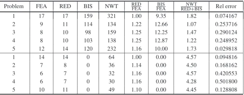
Table 4– Tests with and without the bisection routine for randomly-generated problems with size 100×100. The average running time was 24min for the tests with bisection and 8min for those without bisection.
Problem FEA RED BIS NWT REDFEA FEABIS REDNWT
+BIS Rel error
1 17 17 159 321 1.00 9.35 1.82 0.074167
2 9 11 114 134 1.22 12.66 1.07 0.253716
3 8 10 98 159 1.25 12.25 1.47 0.290124
4 8 10 103 138 1.25 12.87 1.22 0.248952
5 12 14 120 232 1.16 10.00 1.73 0.029818
1 14 14 0 64 1.00 0.00 4.57 0.094816
2 7 8 0 36 1.14 0.00 4.50 0.168162
3 6 7 0 32 1.16 0.00 4.57 0.420553
4 6 7 0 30 1.16 0.00 4.28 0.501800
5 10 11 0 49 1.10 0.00 4.45 0.128808
In Table 1 (problems with size 50×50) it can be seen that problem 3 (with or without bisec-tion) has a high relative error, with a difference of almost 40%. This also applies to problem 5 without bisection. On the other hand, in Table 2 (problems with size 50×100) only problem 2 with bisection shows a high relative error, over 20% of difference. In Table 3 (problems with size 100×50), problem 2 and 4 (with and without bisection) showed the worst relative errors, somewhere around 40% and 20% of difference respectively. Finally, in Table 4 (problems with size 100×100), problems number 2, 3 and 4 (with bisection) also have high relative error, over 20% of difference. It is worth mentioning that for all tables, the number of ACRA calls (FEA) and the number of calls of the reduction procedure (RED) is considerably low when com-pared to the number of calls of the bisection procedure (BIS). As a final comment, we observe that when we compare the number of calls of the Newton method (NWT) for all the 20 test problems considered, the value obtainedwithout bisection is approximately 25% of the value
All problems were solved by computer codes implemented in MATLAB, running on a computer with an Intel Core 2 Duo – E7500, 2.93 GHz processor, with 3.9 GB of usable RAM.
6 CONCLUSIONS
We extended the known results in [5] for the linear case, using smooth convex regions.
We also presented a heuristic (ACRA) able to recover the approximate analytic center when we perturb (through the addition of new constraints) the initial region. It is worth recalling that this is fundamental when we work inside a cutting plane methodology that uses the approximate analytic center as a testing point.
In the sequence, we presented a procedure (CFA) the solves an important problem of applied mathematics, that is, the feasibility problem, using the heuristic ACRA.
Finally, the numerical results presented solving the feasibility problem for randomly-generated problems, show that the greatest number of iterations, due to the bisection routine, represents nearly ten times the calls to the routine ACRA, when we are interested in obtaining an approxi-mation for the analytic center.
It is important to underline that the number of calls to ACRA in the second case, i.e. without the bisection routine, is smaller than when using the bisection routine. On the other hand, in many problems the number of calls to Newton’s method almost duplicates in the second case. Finally, the number of calls to the reduction routine does not show meaningful variation in both cases.
All the tests in this work were carried out using randomly generated problems, mainly because of their easiness and readiness to use. Clearly, every improvement of CFA will depend on more clever ways to define the bisection routine. In the future, with such improvement, we hope to be able to test our heuristic with known library problems.
REFERENCES
[1] BASESCUVL & MITCHELLJE. 2008. An analytic center cutting plane approach for conic program-ming.Mathematics of Operations Research,33: 529–551.
[2] ENGAUA, ANJOSMF & BOMZEI. 2013. Constraint selection in a build-up interior-point cutting-plane method for solving relaxations of the stable-set problem.Mathematical Methods of Operation Research,78: 35–59.
[3] ENGAUA, ANJOSMF & VANNELLIA. 2010. On interior-point warmstarts for linear and combina-torial optimization.SIAM Journal on Optimization,20(4): 1828–1861.
[4] ENGAUA. 2012. Recent Progress in Interior-Point Methods: Cutting-Plane Algorithms and Warm Starts. Handbook on Semidefinite, Conic and Polynomial Optimization. International Series in Operations Research & Management Science,166: 471–498.
[6] GOFFINJL, LUOZ-Q & YEY. 1996. Complexity Analysis of an Interior Cutting Plane Method for Convex Feasibility Problems.SIAM Journal Optimization,6: 638–652.
[7] GONDZIOJ. 2012. Interior Point Methods 25 years later.European Journal of Operational Research, 218: 587–601.
[8] GONDZIO J, GONZALEZ´ BREVIS P & MUNARI P. 2013. New developments in the primal-dual column generation technique.European Journal of Operational Research,224: 41–51.
[9] HORNR & JOHNSONCR. 1985.Matrix Analysis. Cambridge University Press.
[10] HUARDP & LIEU T. 1966. La M`ethode des Centres dans un Espace Topologique.Numerische Mathematik,8: 56–67.
[11] KARMARKARN. 1984. A new polynomial-time algorithm for linear programming.Combinatorica, Berlin,4(2): 373–395.
[12] LIU YZ & CHEN Y. 2010. A Full-Newton Step Infeasible Interior-Point Algorithm for Linear Programming Based on a Special Self-Regular Proximity. The Ninth International Symposium on Operations Research and Its Applications (ISORA’10) Chengdu-Jiuzhaigou, China, pp. 19–23.
[13] MITCHELLJE. 2003.Polynomial interior point cutting plane method. Technical Report, Mathemati-cal Sciences, Rensselaer Polytechnic Institute, Troy, NY, 12180.
[14] MITCHELL JE & RAMASWAMYS. 2000. A Long-Step, Cutting Plane Algorithm for Linear and Convex Programming.Annals of OR,99: 95–122.
[15] NESTEROV YE & NEMIROVSKY AS. 1989. Self-Concordant Functions and Polynomial Time Methods in Convex Programming. SIAM Studies in Applied Mathematics.
[16] ROOSC. 2006. A full-Newton stepO(n)infeasible interior-point algorithm for linear optimization. SIAM J. Optimization,16(4): 1110–1136.
[17] SKAJAAA, ANDERSENED & YEY. 2013. Warm starting the homogeneous and self-dual interior point method for linear and conic quadratic problems.Mathematical Programming Computation,5: 1–25.