MASTER
MATHEMATICAL FINANCE
MASTER
’
S FINAL WORK
D
ISSERTATION
OPTION PRICING UNDER VARIABLE VOLATILITY
C
ATARINA
N
ETO
M
ARQUES
MASTER
MATHEMATICAL FINANCE
MASTER
’
S FINAL WORK
D
ISSERTATION
OPTION PRICING UNDER VARIABLE VOLATILITY
C
ATARINA
N
ETO
M
ARQUES
S
UPERVISIORS
:
J
OÃO
P
AULO
V
ICENTE
J
ANELA
O
NOFRE
A
LVES
S
IMÕES
Resumo
A teoria de valoriza¸c˜ao de op¸c˜oes que conhecemos hoje em dia deu o seu maior passo
quando Fischer Black e Myron Scholes escreveram um artigo com uma f´ormula
fechada que permitia calcular os pre¸cos de op¸c˜oes Europeias de compra e venda
cujo subjacente ´e uma ac¸c˜ao ou um ´ındice. No entanto, evidˆencias mostram que
a f´ormula anterior n˜ao funciona bem num grande n´umero de situa¸c˜oes reais: os
pre¸cos estimados desviam-se significativamente dos pre¸cos de mercado. Isto deve-se
`as hip´oteses, muito restritivas, em que o modelo est´a assente.
Esta disserta¸c˜ao alarga o modelo de Black-Scholes a situa¸c˜oes em que a
volatil-idade do pre¸co do ativo ´e vari´avel. As implica¸c˜oes desta extens˜ao s˜ao estudadas
tanto de um ponto de vista te´orico como pr´atico. Existem muitos modelos
propos-tos para o caso em estudo e este trabalho foca-se nos modelos de volatilidade local
porque mantˆem as caracter´ısticas mais importantes do modelo original. Foram
sele-cionadas quatro fun¸c˜oes diferentes para descrever a volatilidade do pre¸co do ativo e
um m´etodo de diferen¸cas finitas foi implementado para obter estima¸c˜oes e previs˜oes
do pre¸co de op¸c˜oes.
Os resultados obtidos realmente indicam que os modelos de volatilidade local
estimam melhor os pre¸cos das op¸c˜oes do que o modelo de Black-Scholes original.
Palavras-chave:
Valoriza¸c˜ao de op¸c˜oes, Volatilidade local, M´etodo de Crank-Nicolson, Calibra¸c˜ao.The modern theory of option pricing gave its biggest step when Fischer Black and
Myron Scholes wrote a paper with a closed form solution for the prices of European
call and put options on a single stock or index. However, evidence shows that the
former formula no longer holds in many real cases: the estimated prices deviate
significantly from the market ones. This is due to the very restrictive assumptions
on which the model is based.
This dissertation extends the Black-Scholes model by making the volatility of
the asset price variable. The implications of this extension are studied from both
theoretical and practical points of view. Several models have been proposed and this
work focuses on the local volatility models because they maintain the most important
features of the classical model. Four different functions were selected to describe the
volatility of the asset price and a finite difference method was implemented in order
to obtain the estimations and predictions of the option prices.
The results suggest that indeed local volatility models have a better performance
than the classical Black-Scholes model in estimating option prices.
Keywords:
Option Pricing, Local Volatility, Crank-Nicolson scheme, Cal-ibration.Acknowledgments
First of all, I would like to thank my supervisors Prof. Jo˜ao Janela and Prof. Onofre
Sim˜oes for their calm when I was stressed and letting me have the freedom in many of
the decisions taken throughout the dissertation. To all the colleagues I met at ISEG
and accompanied me during this important journey. Also, I would like to thank
my parents and my brothers, who support me not only during my dissertation but
during my whole life. A special thank you to my boyfriend, for the long afternoon
sessions working on the dissertation and the encouragement words when I needed
it.
Contents
Resumo . . . iii
Abstract . . . iv
Acknowledgments . . . v
1 Introduction 1 2 Option Valuation with Variable Volatility 3 2.1 Extensions of the Black-Scholes Model . . . 4
2.2 Local Volatility Functions . . . 6
2.3 Generalized Black-Scholes Equation . . . 8
3 Numerical Methods for Option Pricing 10 3.1 Finite Difference Methods Overview . . . 11
3.1.1 Crank-Nicolson method . . . 14
3.2 Important PDEs Found in Finance . . . 15
3.3 Calibration . . . 18
4 Results 21 4.1 Data . . . 22
4.2 Parameter Calibration and Estimation . . . 23
4.2.1 Black-Scholes model . . . 23
4.2.2 Local Volatility model . . . 24
4.2.3 Model comparison . . . 27
4.3 Prediction . . . 29
5 Conclusions 33
Bibliography 34
A Numerical Code, Data and Parameter Values 37
A.1 C-N method code . . . 37
A.2 Data . . . 39
A.3 Parameter values . . . 41
Chapter 1
Introduction
Since 1973, when the famous paper by Black and Scholes appeared [1], a huge
growth in the options market has been observed. These authors influenced the way
investors saw this market and started the modern theory of option pricing. However,
their model is based on assumptions that clearly do not match reality and evidence
shows that the theoretical prices (prices predicted by Black-Scholes formula) deviate
significantly from the market prices (prices at which options are actually traded).
One of the most important assumptions of this model is that the stock price follows
a geometric Brownian motion with constant volatility, which several authors showed
not to be the case [5,8].
The aim of this dissertation is to build a model closer to reality by relaxing the
constant volatility assumption and allowing for variable volatility in the asset price
dynamics. This modification increases the complexity of the model, leading to a
solution that cannot be obtained in a closed form. This drawback is counterbalanced
by the fact that option prices closer to the market ones are expected to be obtained
even if approximative methods are required.
Several alternatives have been proposed for the generalization of the
Black-Scholes model and most of the literature is based on stochastic volatility [11, 12] and
jump models [10], but we will focus on other type of models, called local volatility
models [7, 9]. These models extend the classical Black-Scholes retaining its most
important features without increasing the degree of uncertainty, in contrast with the
former, which introduce non-traded sources of risk: stochastic volatility and jumps,
Chapter 1. Introduction 2
respectively. The local volatility models are characterized by a Partial Differential
Equation (PDE) that explains the evolution of an option’s price, which has the same
form as the one obtained using classical assumptions. Nevertheless, it generally does
not have an analytical solution, so it will be solved using numerical methods.
One of the most popular methods used in Finance in option problems when
we have to solve a PDE is the Crank-Nicolson scheme [22], well suited for solving
initial boundary value problems (IBVP). This scheme is second order accurate in
time and space, gives good approximations for the solution and is relatively easy to
program. Because of the nature of the chosen problem - a parametric local volatility
model - calibration is needed in order to get the best possible fitting to the data (to
implement the method and calibrate the model, we used MatLab code).
To compare the improved model to the standard Black-Scholes model, the prices
for call options on the S&P 500 Index were estimated and set against the real market
prices. Moreover, using the models that estimated the market prices better than the
Black-Scholes, we tested their performance outside sample to see if the predictions
were good.
The dissertation is structured as follows: Section 2.1 presents the classes of
models found in the literature, concerning extensions of the Black-Scholes model,
in particular the class of local volatility models. Section 2.2 contains the functions
which will be used for the local volatility and in Section 2.3 the Partial differential
equation for the price of an European option with underlying asset following a
gener-alized Geometric Brownian Motion is derived. Chapter 3 is dedicated to the solution
of the PDE presented in Section 2.3. In the first section of this chapter, we describe
the numerical method used, the Crank-Nicolson method. Section 3.2 presents some
PDEs usually found in Finance. The last section presents the calibration problem,
which will allow for the choice of parameters in the functions described in Section
2.2. Chapter 4 describes the market data used and the results obtained. In the
appendix, we can find the code used to implement the Crank-Nicolson scheme. We
can also find the market data and the calibrated parameters for each of the models
Chapter 2
Option Valuation with Variable
Volatility
Although Black and Scholes have influenced the modern theory of option pricing,
the estimated prices using the original formula often quite diverge from the market
ones, which led to several extensions of the classical model. One class of extensions
is concerned with the assumption of constant volatility in the asset price dynamics,
which is of the form
dSt=αStdt+σStdW t,
where α ∈ R is the mean return, σ ∈ R+ is the (local) volatility and Wt is a
standard Wiener process. Using this model, a closed form solution for the price of
an European call (or put) can be derived:
C(S, t) =N(d1)S−Ke−r(T−t)N(d2), (2.1)
wherer is the risk-free rate, K is the strike price,T is the maturity and
d1 = ln(S/K)+(r+σ
2
/2)(T−t)
σ√T−t and d2 =d1−σ
√
T −t.
Under the assumption of constant volatility, it is expected that, when inserting
the market price of a call option into (2.1) with the respective strike and time
to maturity, by solving it with respect to the volatility, the result is constant for
different strikes and maturities. The volatility resulting from this process is called
implied volatility.
Chapter 2. Option Valuation with Variable Volatility 4
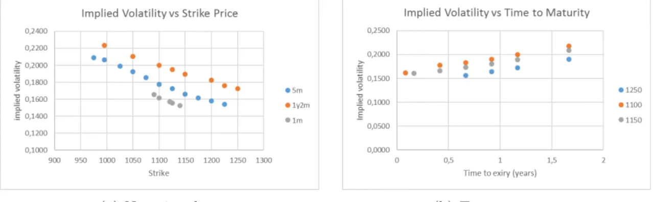
The problem is that, by calculating the implied volatilities, we can observe a
distinguish feature, usually denominated volatility smile: volatility depends both on
strike and time to maturity [5, 8], contradicting the assumption of the Black-Scholes
model. Generally, in stock and index options, it is observed what is called a
neg-ative skew: the implied volatility is a decreasing function of the strike price. The
relationship of the implied volatility with time to maturity is called term structure
and, in general, it is observed that the implied volatility increases with time to
ma-turity. Using data from [18] of 77 call options on the S&P 500 Index and calculating
the corresponding implied volatilities, we can observe the two features described in
Figure 2.1:
(a) Negative skew (b) Term structure
Figure 2.1: Properties of implied volatility
2.1
Extensions of the Black-Scholes Model
In the literature, there are essentially three different classes of extensions concerning
the problem of variable volatility: stochastic volatility models, jump diffusion models
and local volatility models. In this section, we will briefly discuss these alternative
models, particularly the local volatility models.
In stochastic volatility models, as the name implies, the volatility of the asset is
itself assumed to follow a stochastic differential equation, which frequently has some
correlation with the stock price dynamics. This allows for skewness (measure of
asymmetry) and leptokurtic (measure of tail weights) features in the distribution of
the asset, which are many times observed in the market. The pioneers of this type of
this idea to account for the so-called volatility smile observable on option prices.
Heston [11], for instance, used a mean-reverting equation to model the volatility
and obtained a closed form solution for some types of options.
In jump diffusion models, the distribution of the underlying stock return is no
longer continuous and the innovation is the introduction of a jump component in the
asset dynamics, which allows for a positive probability of an abrupt change in the
stock price. Merton [10] associates the appearance of a jump to outliers observed in
stock series as a result of some announcement on the firm. This author highlights
two different variations associated to the change in the stock price: the normal one,
which follows Black-Scholes theory, and the abnormal variations, which arrive at
discrete points in time and have the jump component. This results in a path for the
stock price that is continuous most of the time, but sudden jumps of different sizes
can occur. Finally, to obtain an equation that explains the evolution of the option
price, Merton uses the Capital Asset Pricing Model (CAPM) and the fact that the
jump component represents a non-systematic risk.
These two types of models have a common property: both of them add a new
source of randomness (in the first case, the stochasticity of the volatility and in the
second one, the jump component), which results in an incomplete market and a new
approach must be made in order to find an equation for the option’s price. We say
that a market is complete if every financial derivative can be replicated; because the
sources of uncertainty added in the first two models cannot be traded in the market,
this replication is no longer possible and the completeness is lost (see [22] for a more
precise cover of the topic).
The loss of completeness is not a problem for the local volatility models which
stay close to the original Black-Scholes. The idea behind these kind of models is
quite simple and intuitive: if the implied volatility depends on the strike and
ma-turity of the option, then the local volatility depends on the price of the asset and
on time. Then it can be assumed that the volatility of the asset is a deterministic
function of the two variables, and we continue to have only one source of
uncer-tainty: the Brownian motion in the asset’s price dynamics. In the literature we can
find, primarily, two different approaches: an implicit approach, where the
Chapter 2. Option Valuation with Variable Volatility 6
volatility function assumes a specific form, i.e., an explicit expression is assumed.
This specific function can be fixed or variable in the sense that it has some unknown
parameters that are calibrated using market prices. The first kind of approach was
initiated by Dupire [3], Derman and Kani [8] and Rubinstein [23], who used implied
trees to extract the local volatility function from market data by matching the
theo-retical values of the options with the real ones. However, this exact fit to the current
market data does not perform well when it is applied to predict future prices [4, 5].
Moreover, using this type of models does not give an intuitive explanation for the
volatility function, contrarily to the second approach. Although the parametric local
volatility approach, when calibrated with market data, also does not exactly match
the option prices, it is the strategy chosen for this dissertation because it seems the
best compromise between fitting market data and staying close to the classical BS
model.
2.2
Local Volatility Functions
The work by Dumas, Fleming and Whaley [5] is one of the first attempts at
ex-plaining the local volatility function by giving a specific parametrization toσ(S, t):
these authors tried different quadratic models which resulted in a good fit when
calibrating the parameters for the data used. Nevertheless, it didn’t work outside
the sample: the predicted prices were too different from the real ones. A
num-ber of other researchers contributed with answers to this problem, each one using
a different approach, but always with the same goal in mind: to consider a local
volatility function flexible enough to adjust to the market data (using calibration,
for instance).
Following the work of Hull, Daglish and Suo [4] and Brown and Randall [6], the
functions we have chosen to explain the local volatility of the asset are:
σ(S, t) = a0+a1ln(S/S0) +a2ln(S/S0)2+a3(T −t)
+a4(T −t)2+a5ln(S/S0)(T −t)
(2.2)
σ(S, t) = b0+b1
ln(S/S0) √
T −t +b2
ln(S/S0) √
T −t
2
+b3
ln(S/S0) √
T −t 3
σ(S, t) =c0+c1
ln(S/S0)
(T −t)d0 +c2
ln(S/S0)
(T −t)d0
2
+c3
ln(S/S0)
(T −t)d0
3
(2.4)
σ(S, t) = σAT M(t) +σskew(t)tanh(γskew(t)ln(S/S0)−θskew(t))
σsmile(t) (1−sech(γsmile(t)ln(S/S0)−θsmile(t)))
(2.5)
Functions (2.2)-(2.4) are based on a set of rules of thumb proposed by investors
and/or traders about the implied volatility surface. The authors [4] divide these
rules in three classes: the strike rule, where the implied volatility is assumed to be
independent of the asset price; the delta rule, where the implied volatility depends
on the moneyness variableK/S; and the square root of time rule, where the implied
volatility depends on time trough the square root of time left to maturity. Consulting
the results found by the authors, we conclude that the first rule gives worse results
compared to the other rules, so we do not insert any function concerning it.
In the last function (2.5), all functions σ, γ and θ are of the form β1+β2t
1+β3 , with
different parameters each. As the names appeal,σAT M describes the term structure
of at-the-money volatilities, and the functions withskew andsmile subscript account
for the skew and smile components, respectively. Besides that,σ,γ andθ associated
to these two components give the magnitude, width and centre, respectively, of the
skew and smile. The functions chosen hyperbolic tangent and hyperbolic secant
-are based on the properties expected for the local volatility. The authors [6] state
that, when pricing European options on stocks or indexes, making σsmile(t) = 0
captures most of the behaviour and we do not need the extra parameters given by
the last term on (2.5). Because a parsimonious model is preferable, when applying
to market data, first we will use the model making the above adjustment and then,
if the results are not as good as expected, the extra parameters will be added.
The parameters of the functions above are determined by calibration using
avail-able market data and we will study the estimation and prediction quality of the
models by comparing the option prices that they supply with the real ones in and
outside sample. This study will take place in Chapter 4 with a theoretical framework
Chapter 2. Option Valuation with Variable Volatility 8
2.3
Generalized Black-Scholes Equation
The Black-Scholes model is based on a world where we have a non-dividend paying
stock, denoted bySt, and a risk-free asset, which will be denoted by Bt. Following
[2], we will present a generalized Partial differential equation (PDE) where these
assets can be characterized by the following dynamics:
dBt=rBtdt
dSt=αStdt+σ(St, t)StdW t
(2.6)
where Wt is a standard Wiener process and the asset price follows a lognormal
distribution with meanα and (local) volatility σ(S, t). Also, r is the risk-free rate.
The only difference between the classical Black-Scholes and this generalized
model is that the volatility of the stock price is non-constant, the remaining
as-sumptions are maintained.
The derivation of the PDE consists in setting a riskless portfolio composed by
a long position on an option and some amount on the respective underlying asset.
This amount is chosen in such a way that the resulting portfolio is risk free or, in
other terms, the dWt term vanishes. Then, we will use the proposition below and
the resulting PDE is easily obtained.
Proposition 1. Suppose that there exists a portfolio such that the value process U
has the dynamics
dU =kU dt, (2.7)
where k is a constant. Then, either k = r, or there exists an arbitrage possibility,
where r is the same as in (2.6).
Let V(t, St) be the price of an European option on the stock St at time t. The
option and the stock are affected by the same source of uncertainty (movements in
the stock price, in particular the Wiener process driving the stock’s stochastic
dif-ferential equation), so we can create a riskless portfolio consisting of a long position
on the option and a short amount ∂V
price of that portfolio at timet,
Πt=V(t, S)−
∂V ∂SS.
Using Itˆo’s formula onV(t, S), the infinitesimal change on the price of the portfolio
is given by
dΠt=
∂V
∂t +
1
2σ(t, S)
2S2∂2V
∂S2
dt.
We can see that the choice of the amount of stock in the portfolio made the Wt
term disappear from the portfolio’s dynamics, eliminating the risk. This kind of
manipulation is called delta hedging and must be performed continuously so that
the portfolio is immune to changes in the stock price.
Without randomness in the portfolio, its dynamics must be equal to the one of
the riskless asset or there will exist arbitrage opportunities, according to Proposition
1. Therefore, using (2.7), we have
∂V ∂t +
1
2σ(t, S)
2S2∂2V
∂S2 =r
V − ∂V ∂SS
.
Rearranging the terms, we get the equation,
∂V
∂t (t, S) +
1
2σ(t, S)
2S2∂2V
∂S2(t, S) +rS
∂V
∂S(t, S)−rV(t, S) = 0. (2.8)
Equation (2.8) is theGeneralized Black-Scholes Partial Differential Equation. In
order to get the full problem we need to add extra conditions that will depend on
the type of option to be priced, i.e, if it is a call or a put option.
Even though it seems that this PDE is not that different from the one found on
[1], in general, it has no closed form solution, so it needs to be solved numerically
Chapter 3
Numerical Methods for Option
Pricing
When the option pricing models become more complex, it has been discussed that
it is no longer possible to obtain analytical solutions and numerical ones have to
be found. In the literature, there are three classes of methods that often appear:
tree-based methods, Monte Carlo method and finite difference methods [16, 22, 24].
Tree-based methods rely on the assumption that the stock price, in the next
time step, will have a known number of possible values with given probabilities (in
the case of binomial trees we have two possibilities, trinomial trees display three
possibilities, etc.); then a tree of these stock prices is build until the maturity of the
option. At the maturity, the value of the option is known and, from there, at each
node of the tree, the price of the option is calculated backwards by discounting the
expected value of the option prices in the nodes ahead.
Monte Carlo is a simulation method. It repeatedly generates sample paths of the
underlying, assuming a lognormal distribution for the asset price. This generation
is done until expiry, where we can have an estimated value for the option. Then, we
take the average of all the estimations for the option price and discount it back to
the present.
Finite Difference methods are applied when one needs to solve numerically a
Partial differential equation. These methods convert the PDE into a system of
linear equations by replacing the derivatives with the respective finite difference
approximations.
Monte Carlo method converges slowly (we may need to run it many times until
we get a good approximation, resulting in a high computational cost), which makes
it an undesirable choice. However, when we have an option based on more than two
assets, it becomes more efficient [24, 25] and is widely used in such cases. Although
simple and easy to implement, tree methods also converge at a slow rate. Finite
Difference methods are efficient when dealing with options based on a single asset
[24], which is a plus comparing with the former methods. Moreover, it is easy to
program and handles well coefficients that are time and/or space dependent as in
(2.8). The advantages provided by this method are the reason why it will be the
one used to estimate the option prices in Chapter 4.
The problem one wants to solve is the following:
Find a function u(x, t) :D→R, withD= [A, B]×[0, T] satisfying:
−∂u
∂t +a(x, t) ∂2u
∂x2 +b(x, t)
∂u
∂x +c(x, t)u=f(x, t)in intD (3.1) u(x,0) = u0(x), x∈[A, B] (3.2)
u(A, t) =g0(t), u(B, t) =g1(t), t∈[0, T] (3.3)
This type of problem is usually called a reaction-advection-diffusion problem.
Func-tions a(x, t), b(x, t) and c(x, t) are associated to diffusion, advection and reaction
coefficients, respectively. It has an initial condition and Dirichlet boundary
condi-tions.
3.1
Finite Difference Methods Overview
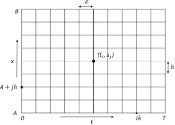
The first step when dealing with finite difference methods is to discretize the domain
both in time and space, resulting in a uniform grid:
• In time: divide [0, T] intoN equally spaced intervals 0 =t0 < t1 < ... < tN =
T, with lengthk= T
N, resulting inN+1 points, denoted byti =ik, i= 0, ...N;
• In space: divide [A, B] into M equally spaced intervals A = x0 < x1 <
Chapter 3. Numerical Methods for Option Pricing 12
xj =A+jh, j = 0, ..., M.
A generic node at the grid is identified by the indices i and j as (ti, xj). This
discretization results in a grid with (N+ 1)×(M + 1) points as in Figure 3.1. The aim of this method is to approximate the functionu(x, t) at these grid-points.
Figure 3.1: Space-time discretization
There are three classic finite difference methods usually applied to IBVPs such
as (3.1)-(3.3): Euler explicit scheme, Euler implicit scheme and Crank-Nicolson
scheme. The explicit scheme is the simplest one, but it has the disadvantage of being
conditionally stable, that is, its stability depends onhand k and their relationship,
more precisely, k/h2 must be less than a certain constant. Using this scheme, for
each time step, we obtain explicitly the value of a grid-point (xi, tj+1) using three
values of the previous time step: (xi−1, tj), (xi, tj) and (xi+1, tj).
If a scheme is not stable, the numerical error tends to accumulate as we go
further in time and we cannot guarantee that it remains bounded. This problem is
handled using implicit schemes. The implicit Euler method is unconditionally stable
and the value of a grid-point (xi, tj) is obtained using three values of the next time
step: (xi−1, tj+1), (xi, tj+1) and (xi+1, tj+1). Here, an explicitly relation cannot be
achieved and a linear system of equations needs to be solved at each time step.
Finally, the Crank-Nicolson scheme is an average of the two previous schemes
and has the advantage of being second order accurate in both thexandtdirections,
order in the t direction [13]. Hence, Crank-Nicolson method is the most precise of
the three and this is the reason why is the one used in the dissertation.
As already mentioned, in this methods we deal with differences instead of
deriva-tives. By Taylor’s expansion, we can write to some function φ(x, t):
φ(x±h, t) = φ(x, t)±h∂φ
∂x(x, t) + h2
2
∂2φ
∂x2(x, t)±
h3
6
∂3φ
∂x3(η±, t)
φ(x, t+k) =φ(x, t) +k∂φ
∂t(x, t) + k2
2
∂2φ
∂t2(x, υ)
with η+ ∈(x, x+h), η− ∈(x−h, x) andυ ∈(t, t+k).
Rearranging the terms, we get the following:
D+φ(x, t)≡
φ(x, t+k)−φ(x, t)
k =
∂φ
∂t(x, t) +O(k) (3.4) D+D−φ(x, t)≡
φ(x+h, t)−2φ(x, t) +φ(x−h, t)
h2 =
∂2φ
∂x2(x, t) +O(h
2) (3.5)
D0φ(x, t)≡
φ(x+h, t)−φ(x−h, t)
2h =
∂φ
∂x(x, t) +O(h
2) (3.6)
(3.4) is called aforward difference approximation and is a first order approximation
to the first derivative ofφwith respect to (w.r.t.) t. (3.6) is called acentre difference
approximation and is a second order approximation to the first derivative ofφw.r.t.
x. Finally, (3.5) is a second order approximation to the second derivative ofφw.r.t.
x.
Then, we have the following approximations of the derivatives in (3.1):
∂φ
∂t(x, t)≈
φ(x, t+k)−φ(x, t)
k ∂2φ
∂x2(x, t)≈
φ(x+h, t)−2φ(x, t) +φ(x−h, t)
h2
∂φ
∂x(x, t)≈
φ(x+h, t)−φ(x−h, t)
2h ,
which can provide approximate values for ∂φ∂t, ∂∂x2φ2 and
∂φ
∂x at any grid point, given
Chapter 3. Numerical Methods for Option Pricing 14
3.1.1
Crank-Nicolson method
At this point, the goal is to convert the continuous problem (3.1)-(3.3) to the
cor-responding discrete version based on the Crank-Nicolson method. We begin by
enumerating some properties of this scheme:
• Consistency: It is consistent. This means that the finite difference represen-tation converges to the PDE as h and k tend to zero;
• Stability: It is unconditionally stable with respect to h and k, i.e., for any choice of these two steps, the error remains bounded;
• Convergence: It is convergent, i.e, the numerical solution tends to the exact solution when N, M → ∞;
• Accuracy: It has a second order accuracy with respect to both x and t, i.e.,
|τi
j| ≤ C(h2 +k2), where C is a constant and τji is the truncation error (see
[13]). The order in x comes directly from (3.5) and (3.6); because this scheme
is evaluated at 12(ti+ti+1), using a centre difference approximation to the first
derivative of u w.r.t t, we get an order of two in time as well.
The notation in this section follows Duffy [14]. Let Lk
h be the discrete operator
defined at the grid-points. One wants to approximate the functionu(x, t) :D→R, with D= [A, B]×[0, T] at the grid-points, that is, to find ui
j =u(xj, ti) such that:
− u
i+1
j −uij
k +
1 2(L
k
huij +Lkhuij+1) =f i+1/2
j , i= 1, ..., N −1, j = 1, ..., M −1 (3.7)
u0j =u0(xj), j = 0, ..., M (3.8)
ui0 =g0(ti), uMi =g1(ti), i= 1, ..., N , (3.9)
whereLk
huij =aijD+D−uij+bijD0uij+cijuij,aij =a(xj, ti),bij =b(xj, ti),cij =c(xj, ti),
fi
j =f(xj, ti), with functions a,b,c and f the same as in (3.1) and
D+D−uij =
uij+1−2uij+uij−1
h2 ,
D0uij =
ui
j+1−uij−1
The system (3.7)-(3.9) does not give an intuitive idea of how we can get the values
of u at the grid-points, but we can transform it into a system of linear equations.
Expanding (3.7), we get
− u
i+1
j −uij
k +
1 2
aiju
i
j+1−2uij +uij−1
h2 +b
i j
ui
j+1−uij−1
2h +c
i juij
+1 2 a
i+1
j
uji+1+1−2uji+1+uij+1−1 h2 +b
i+1
j
uij+1+1−uij+1−1
2h +c
i+1
j uij+1
!
=fji+1/2.
Rearranging the terms and multiplying by 4h2k, it follows
Aiuij+1+1+Biuji+1+Ciuij+1−1 =Di ,
whereAi = 2kaij+1+hkbji+1,Bi =−4h2−4kaji+1+2h2kcij+1,Ci = 2kaij+1−hkbij+1and
Di =−[uij+1(2kaij+hkbij) +uij(4h2−4kaij+ 2h2cij) +uij−1(2kaij−hkbij)] + 4h2kf i+1/2
j ,
fori∈ {1, ...N}and j ∈ {1, ..., M}.
Specifically, starting with a given initial condition, we obtain the solution at the
next time step by solving the following linear system:
1 0 0 . . . 0
C1 B1 A1 0 . . . 0
0 C2 B2 A2 . . . 0
0 0 . .. . .. . .. 0
0 . . . 0 CM−1 BM−1 AM−1
0 0 0 . . . 0 1
ui0+1 ui1+1 ui2+1
...
uiM+1−1 uiM+1
= D0 D1 D2 ...
DM−1
DM
The matrix on the left side is a (M+ 1)×(M + 1) matrix and D0 and DM are the
boundary conditions atx=A and x=B, respectively.
To implement the Crank-Nicolson method we used MatLab. The code for the
general system of equations (3.1)-(3.3) can be found in A1.
3.2
Important PDEs Found in Finance
This overview of some numerical methods had the goal of solving Equation (2.8).
Chapter 3. Numerical Methods for Option Pricing 16
In the case of European vanilla call and put options, denoting the price of the put
byP(S, t), we have the conditions:
C(S, T) =max(S−K,0), P(S, T) =max(K−S,0) (3.10)
C(0, t) = 0, P(0, t) =Ke−r(T−t) (3.11)
C(S, t)→S−Ke−r(T−t), P(S, t)→0as S → ∞ (3.12)
Comparing (2.8) plus the complementary conditions (3.10)-(3.12) with problem
(3.1)-(3.3), there are two differences: the first is the fact that, in the option problem,
we have a terminal condition while in the generalized problem we have an initial
condition; the second is that, in the option problem, the domain of the variable S
is infinite and in the generalized problem the domain is bounded. So, one needs
to make some adjustments in the options problem in order to solve it using C-N
method: truncate the domain of S and perform a change of variables so that t
denotes time left to maturity and not maturity itself.
Artificially truncating the domain of the asset price implies an additional error
to the finite difference scheme. To attenuate the effect of this error, one must choose
the maximum value of the asset price - let Smax be that value - far enough of the
so called region of interest, but not too far as to bring a lot of computer effort.
Investigations from [20] and [21] suggest a value of about three to four times the
highest strike of the market data available.
In the next subsections, three examples of Partial differential equations
com-monly found in Finance are given. These PDEs are going to be used to get the
estimated prices of options that we then use to compare with the market prices.
The choice of the PDE we will use to estimate the prices will depend on the type of
data used.
Forward PDE
In this first adjustment, we will truncate the domain in the variable S as [0, Smax].
The following change of variable is done: t∗ =T−t, where t∗ stands for time left to
have
∂V∗
∂t∗ =
∂V ∂t
∂t ∂t∗ =−
∂V ∂t .
Replacing this derivative in (2.8) and returning to the original variable names, i.e.,
tand V(S, t) denoting time to maturity and price of the option, respectively, we get
the new PDE (with respective conditions) in the call case:
−∂V∂t + 1
2σ(t, S)
2S2∂2V
∂S2 +rS
∂V
∂S −rV = 0, t∈(0, T), S∈(0, Smax) V(S,0) = max(S−K,0)
V(0, t) = 0, V(Smax, t) = S−Ke−rt
This is called a forward Partial Differential Equation.
Logarithmic PDE
In this second adjustment, we will perform two changes of variables: t∗ =T−t and
x =log(S). The first one is exactly the same as above, the second transforms the
prices into its logarithm. Now, the resulting function is V′(x, t∗) = V(ex, T −t∗)
and we calculate the derivatives:
∂V′
∂t∗ =
∂V ∂t
∂t ∂t∗ =−
∂V ∂t ∂V′ ∂x = ∂V ∂S ∂S ∂x =S
∂V ∂S ∂2V′
∂x2 =S
∂V ∂S +S
∂2V
∂S2
∂S ∂x =S
∂V ∂S +S
2∂2V
∂S2.
In this case, the domain of the variable x is truncated as (xmin, xmax), where xmin
no longer needs to be zero. Now, again denoting t as time left to maturity, we can
write the PDE (with respective conditions) for a call option:
−∂V∂t + 1 2σ(x, t)
2∂2V
∂x2 +
r− 1
2σ(x, t)
2
∂V
∂x −rV = 0, t∈(0, T), x∈(xmin, xmax) V(x,0) = max(ex−K,0)
Chapter 3. Numerical Methods for Option Pricing 18
According to [13], when pricing vanilla options, the choice between these two
PDEs does not affect the solution in a significant way, what really matters is to use
a suitable grid.
Dupire PDE
Here, we are going to present a particular Partial Differential Equation for a call
option as a function of strike and time to maturity,C(K, T), derived by Dupire, see
[13]. Fixingt= 0 and denoting the spot price by S0, the price of a call option must
satisfy the following PDE:
− ∂C
∂T +
1
2σ(K, T)
2K2∂2C
∂K2 −rK
∂C
∂K = 0, T ∈(0, Tmax), K ∈(0, Kmax) C(K,0) =max(S0 −K,0)
C(0, T) = S0, C(Kmax, T) = 0
This equation is called Dupire PDE and allows to price call options with various
strikes and maturities on the same underlying asset.
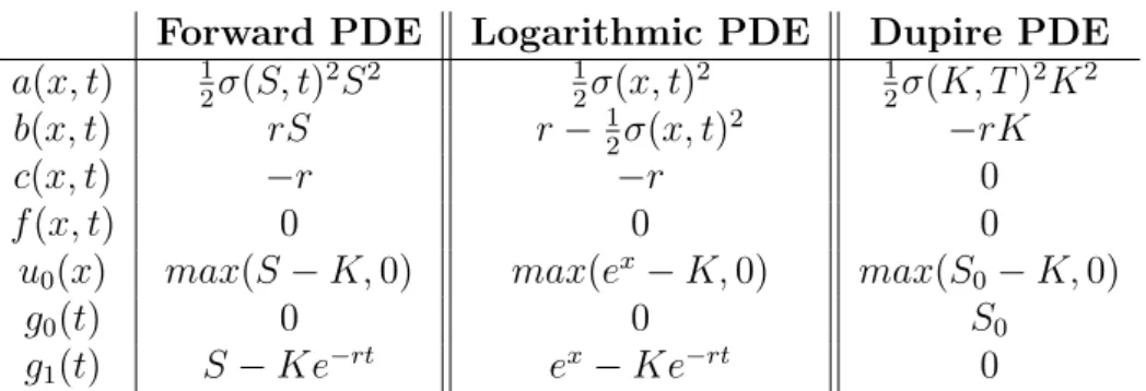
Comparing the three Partial Differential Equations above with problem
(3.1)-(3.3), the generic coefficient and respective conditions become:
Forward PDE Logarithmic PDE Dupire PDE
a(x, t) 12σ(S, t)2S2 1
2σ(x, t)2
1
2σ(K, T)2K2
b(x, t) rS r− 1
2σ(x, t)
2 −rK
c(x, t) −r −r 0
f(x, t) 0 0 0
u0(x) max(S−K,0) max(ex−K,0) max(S0−K,0)
g0(t) 0 0 S0
g1(t) S−Ke−rt ex−Ke−rt 0
Table 3.1: PDEs found in Finance
3.3
Calibration
Model calibration can be defined as the process of fitting models to market data.
These models can depend on some unknown parameters (as the local volatility
from the market. The aim is to choose the parameters in such a way that the
estimated prices are as close as possible to the market prices. The term close has
no unique definition, it will depend on the problem formulated, particularly, on the
function chosen to minimize the differences.
In general, the first step when one wants to calibrate a model is to choose which
function (generally called objective function) will be minimized and, once this
de-cision is made, choose which optimization process will be used to minimize the
objective function.
One way to solve the calibration problem is via least squares formulation. Least
squares are broadly discussed in the literature [22] in its linear form, but the structure
of our problem excludes this possibility, so we have to work with nonlinear least
squares. Even though this form can fit a wide range of functions, it has the following
disadvantage: an iterative algorithm needs to be used in order to get the parameter
estimates. Besides the fact that the implementation is harder than in the linear
case (where the solution can be found analytically), this kind of methods are not
flawless, that is, they strongly depend on the initial solution, and more than one
stopping condition must be imposed so that the algorithm terminates, even if an
optimum is not reached. Nevertheless, theory behind non linear least squares is well
developed [26] and MatLab has an incorporated function which handles this kind
of problems. From now on, we will only talk about nonlinear least squares. The
procedure consists in finding the best fitting to a given set of points by minimizing
the sum of squares of the offsets of the points from the fitted values, i.e., find the
coefficient a∈Rp which solves the problem of finding:
argmin
a n
X
i=1
[yi(a)−ydatai]2
This method can be extended so it handles restrictions on the search domain for
a= (a1, ..., ap).
The MatLab function to solve such problems works, summarily, in this way [29]:
1. Starts with an initial estimate for each coefficient, called initial solution;
Chapter 3. Numerical Methods for Option Pricing 20
3. Adjusts the coefficients and determines whether the fit improves. The function
has five different algorithm choices and the default one can solve most of the
problems, so that’s the one which will be used;
4. Iterate the process by returning to step 2 until the fit reaches the specific
convergence criteria. The convergence criteria has four types of situations:
function converges to a solution; change in the solution is less than a certain
value; change in the residual is less than a certain value; or magnitude of search
direction is smaller than a pre-established value.
For the choice of initial solution in step 1, if we do not have any prior information
that could give us an intuition about it, we should generate many sets of initial
values and select the one that leads to a better solution (in our case, the solution
which has the lowest value).
Local Volatility Model
In our particular case, i.e., in the local volatility model, is quite straightforward that
each choice of parameters for σ(t, S), fixing one of the functions (2.2)-(2.5), gives
a different solution to the option value, so one needs to estimate the parameters
that give the minimum value for the sum of the squared differences between the
estimated price and the observable one. Our problem is of the type:
arg min
a∈Rp
n
X
i=1
[V(Ki, Ti;a)−Vi∗]2 (3.13)
s.t. σ(t, S;a)≥0 (3.14)
wherenis the number of market observations,V is the price estimated by the model
with strikeKi, maturity Ti, and volatility parametera, andV∗ is the market value
for the same strike and maturity. The data used in this problem consists of a family
of vanilla call or put options with different strikes and maturities on some underlying
Chapter 4
Results
To get the results searched for this dissertation, one needs to do the following: for
each local volatility function defined in Chapter 2, calculate the estimated prices for
a call or put option using the Crank-Nicolson scheme, choosing one of the PDEs in
Section 3.3. This method will return a grid where each point defines an option price
for a given maturity and strike.
The grid constructed is uniform (see Figure 3.1), so the prices of the options
produced by the Crank-Nicolson method will have strikes and times left to maturity
evenly spaced. The probability of getting option data which lies in these exact points
is low, so we need to find a way to deal with this problem. It can be overcome by
using interpolation between the values calculated at the grid points: according to
[20] and [21] a cubic spline interpolation should be sufficient as it will not affect the
error in a significant way.
After interpolating the estimated data, we are ready for the calibration by just
using the MatLab function to minimize the sum of the squared differences between
the interpolated data and the market one, subject to the constrain that the local
volatility must be non-negative (problem (3.13)-(3.14)). Once we have all the
pa-rameters for each local volatility function, we can compare the results to see which
model(s) seems more suitable and if it is really an improvement over the standard
Black-Scholes. Besides that, we should also see if the qualitative properties showed
in Figure 2.1 for the local volatility are preserved.
From the beginning of this work, it is clear that the only difference between the
Chapter 4. Results 22
local volatility model and the standard Black-Scholes model is the assumption of
constant volatility. This modification is made in order to get closer to reality and
hence to improve the capacity of estimation of the BS model; therefore, throughout
the next sections, we will start by giving the results using the standard Black-Scholes
model and then will use these values to assess the quality of the new models.
4.1
Data
The market data used in this dissertation consists of call options whose underlying
is the S&P 500 Index. This decision was made based on the amount of options
traded daily on this Index and, since more trades give a better perspective of the
market, we chose one of the most active options in the market. From the various
strikes and maturities available, 86 options were chosen with strike prices varying
from 2150$ to 2650$ and time left to maturity from 8 days to 638 days (March 2017
to December 2018). These options were taken on 23 March 2017 and at the close
of the market the S&P 500 Index was worth 2345.96$. It is a common practice
to work with midprices (see [22] for instance), that is, the average between the bid
(maximum price that a buyer is willing to pay) and ask (minimum price that a seller
is willing to receive) prices:
Ci =
Cask
i +Cibid
2 .
The midprices for the 86 call options and a plot of the prices against strike can be
found in Appendix A.2.
Both the Forward PDE and the Logarithmic PDE presented in Section 3.2 are
used to obtain the price of an option where the strike is fixed and the asset price
is variable. Since our data consists of points of the form (Ki,Ti), where Ki is the
strike andTi is the time left to maturity of the ith option, respectively, it seems that
the Dupire PDE is the most suitable choice, because it treats the call option as a
function of both strike and time left to maturity.
To get all the data for the calculation of the option prices, we still need one more
element: the risk-free rate. This value is defined as the return of an investment with
some risk, even if it is insignificant. Frequently, government security rates are used
as a proxy for risk-free rates, either short-term or long-term [27]. In practice, it is
common to use the interest rate on a three-month U.S. Treasury Bill as a proxy for
the risk-free rate, and we will follow it. From the U.S. Department of the Treasury
[28] was possible to recover the T-Bill rates on 23 March 2017. In Table 4.1, we can
observe the values for different time horizons.
4 Weeks 13 Weeks 26 Weeks 52 Weeks
0.72 0.75 0.88 0.95
Table 4.1: Treasury Bill Rates on 23 March 2017 (%)
Reading the table and taking into account the usual practice, we obtain a
risk-free rate of 0.75% (75 basis points).
4.2
Parameter Calibration and Estimation
In the next sections we will present the results of the calibration of the standard
Black-Scholes model and the local volatility model, using the dataset described in
the previous section. All four functions for the volatility are used, so we will end with
four different estimations plus the Black-Scholes estimation for the option prices.
The comparison between the different models and the market prices will have two
components: a “numerical” one, using different measures to describe the goodness
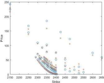
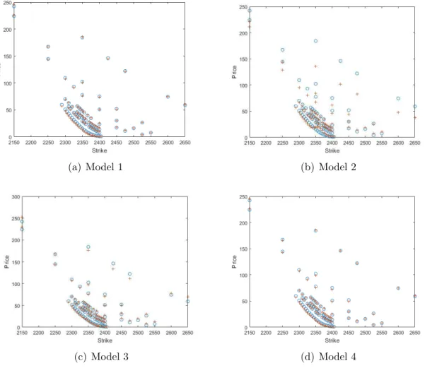
of the fit, and a “visual” one, where we plot the market prices against the model
ones. In this plot, the market prices are denoted by a blue circle and the model
prices by a red plus sign. The goal is to calibrate the models in such a way that the
plus signs and the circles overlap or stay as close as possible.
4.2.1
Black-Scholes model
Using the Black-Scholes formula for call options (2.1) to estimate the option prices
and stating the volatility parameterσ as the unknown parameter which needs to be
calibrated, we get a value ofσ = 11.79%. This is the value which gives the best fit
by minimizing the squared differences between the BS prices and the market ones
Chapter 4. Results 24
Although for the shorter maturities the estimation is accurate, we observe that,
as the maturity increases, there is a big discrepancy between the estimated and the
market prices. This evidence is expected and backs up what was mentioned on the
introduction regarding the quality of the BS model in market price estimation.
Figure 4.1: Market Pricesvs. Black Scholes estimation
4.2.2
Local Volatility model
At this point, we will make a parameter calibration using the four different local
volatility functions (2.2)-(2.5). The variable t is defined in years and varies from 0
to 2.5 to include all the maturities of the data. The variable K varies from 0 to
8000.
Using the procedure already described at the beginning of this chapter, we made
some experiments using different steps (time and space) on the Crank-Nicolson
method and different starting points for the minimization of the objective function.
Changing the time and space steps of the scheme does not change the magnitude
of the results, that is, it increases or decreases the value of the objective function
but not in a significant way. The running time of the program (computational time)
didn’t change much using bigger or smaller steps, so we decided to use M = 400
and N = 100, withM and N having the same notation as in Chapter 3. The same
cannot be said about the starting points: in all models, except Model 1, a different
started at different starting points and kept the solution which gave the lowest value
for the objective function. This behaviour can be associated to the existence of local
minimum points.
For the first function (2.2), we can find the value of the calibrated parameters
in Table A.2 in the Appendix. Looking at Figure 4.2 (a), we can see that there
exists a big improvement over the Black-Scholes model as the estimated prices are
closer to the real ones, particularly at longer maturities, which were the ones where
the Black-Scholes estimation was less accurate. For almost all the prices the crosses
are inside the circles, i.e, there exists an overlap between estimated and real prices,
which is the aim when one uses a model to describe the options market.
(a) Model 1 (b) Model 2
(c) Model 3 (d) Model 4
Figure 4.2: Market prices vs. model estimations
For the second function (2.3) the same didn’t happen. The estimated prices are
even further from the real ones when we compare them to the BS estimation. This
Chapter 4. Results 26
Figure 4.2 (b), which is where this models seems to fail more. The parameters values
can be found in the Appendix, Table A.3.
The third function (2.4) is an extension of the previous one. The only difference
is an extra parameter which gives more flexibility, hence we expect this model to
give better results than the second. This is indeed true, there exists an improvement
over Model 2 and even more, this improvement extends to the BS model. Comparing
Figure 4.2 (c) and Figure 4.1, we can see that the prices estimated by this model
are closer to the real ones. Nevertheless, there are still some prices that are far from
the market ones. The parameters can be found in Table A.4.
The fourth function (2.5) produces Figure 4.2 (d), where we can observe an
improvement over the Black-Scholes estimation. It seems that this model had a
better performance than the third in estimating the option prices (particularly at
longer maturities) and the results are similar to the ones produced by Model 1. The
parameters can be found in Table A.5.
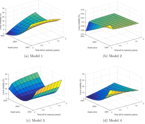
With the parameters obtained from the calibration, we can construct the local
volatility surface for each function. Figure 4.3 shows the local volatility as a function
of time left to maturity and asset price and its values are in percentage.
The local volatility surface generated by Model 1 in Figure 4.3 (a) shows, in
overall, the properties expected for the local volatility: as the asset price decreases
its value increases and increases as the maturity rises. For the longest maturity,
there is an exception: the volatility decreases a little before it starts increasing.
Observing Figure 4.3 (b), we can see that for the second model the volatility is
practically plain in the domain under consideration. This means that, even
consid-ering a deterministic function for the volatility, when we calibrate the parameters,
the volatility becomes constant, in this case, with a value around 10%. For the third
model, the relationship of the volatility with maturity follows the expected pattern,
i.e., it increases as the maturity increases. For the relationship with the asset price,
the shape is not what we excepted, instead it is a U-shape. Finally, observing Figure
4.3 (d) we can see that Model 4 shows, in overall, the features we expected, with
one exception. For small values of the asset price, the volatility decreases when the
maturity increases, which contradicts the properties seen in Figure 2.1.
(a) Model 1 (b) Model 2
(c) Model 3 (d) Model 4
Figure 4.3: Local volatility surface for each model
better than Black-Scholes in estimating the option prices. As for models 1, 3 and 4,
we saw a substantial improvement as they seem to estimate the market prices much
better than the standard BS model.
4.2.3
Model comparison
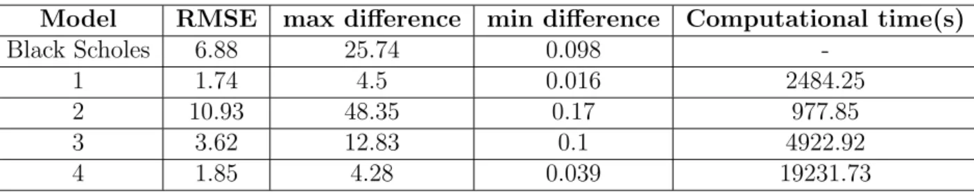
For comparative purposes, we will use a measure proposed in [18], which estimates
the goodness of fit. It is called root-mean-squared-error (RMSE) and is given by:
RM SE =
v u u t
N
X
i=1
(market pricei − model pricei)2
N ,
where N denotes the number of options. Moreover, we also register the
compu-tational times because they are an important parameter when comparing models
maxi-Chapter 4. Results 28
Model RMSE max difference min difference Computational time(s)
Black Scholes 6.88 25.74 0.098
-1 1.74 4.5 0.016 2484.25
2 10.93 48.35 0.17 977.85
3 3.62 12.83 0.1 4922.92
4 1.85 4.28 0.039 19231.73
Table 4.2: Comparison between various models
mum and minimum difference between real and estimated prices (in absolute value),
Table 4.2 was obtained.
Observing Table 4.2, the measures obtained support what we noticed in the
previous section. Comparing the values of the RMSE with the one for the
Black-Scholes model, we can see that for the first model it decreases to approximately
a quarter of the value, which is consistent with Figure 4.2 (a). Besides that, the
minimum and maximum differences are less than what we have for the Black-Scholes,
emphasizing that the larger difference for the BS model is more than five times what
we have for the first model. For Model 2, as we expected from the Section 4.2.2, the
values we get are the worst considering all the models explored in this dissertation.
The RMSE is almost twice the value in the BS model as well as the maximum
difference between the estimated and the real prices. Model 3 shows an improvement
over the Black-Scholes model: the RMSE reduces to approximately half the value
of the BS model and the maximum difference between the estimated and market
prices also decreases considerably. Between Model 4 and Model 1, there is not much
difference: the RMSE is similar for the two models as well as the maximum and
minimum differences found among the prices. These two models are the ones with
better results.
However, so far we haven’t considered the last column of the table, which is
important to compare models 1, 3 and 4, the ones that performed better than the
standard model. Model 1 takes 2484.25 seconds ≈ 41.4 minutes to calibrate the parameters, Model 3 takes 4922.92 seconds ≈ 82 minutes ≈ 1.37 hours and Model 4 takes 19231.73 seconds ≈ 320.53 minutes ≈ 5.34 hours (on average). As we can see, Model 4 consumes much more time than the other two models to calibrate the
that takes less time to calibrate the parameters and combining this with the results
observed in Table 4.2, we can conclude that this model is the best among all the
models.
To finalize, observing all the results obtained for the local volatility models
con-sidered and the comparisons made between them and the original Black-Scholes
model, the second one is not a good model because it doesn’t estimate the prices
better than the standard model. The first, second and fourth models are an
im-provement over the Black-Scholes, with Model 1 performing better than the others,
considering both the numerical results and computational times.
4.3
Prediction
In this section, another property of the models will be studied: we will check if the
local volatility models used in the previous section are good predictors, i.e., we will
study the ability of the models to predict prices outside sample. The procedure is
done in the following way: we calibrate the model considering a certain sub-sample
of the data and then predict the prices outside that same sub-sample. Given the
conclusions made in the previous sections, we will only perform the described for
models 1, 3 and 4.
To study this feature, we distinguish two different sub-samples of the original
dataset:
• All strikes from the shorter maturity until 21 July 2017;
• All maturities with strike varying from 2305 to 2395.
These sub-samples were chosen in a way to balance the number of options that will be
calibrated and those that will be used for forecasting. We should have more options
in the calibration procedure, but we cannot have few in the forecast, otherwise this
would affect the purpose of this study.
Replicating the strategy of the previous sections, the values of the parameters
(for the two sub-samples) for the models can be found in the Appendix. Comparing
the values of the calibration for the whole sample and for each of the sub-samples,
Chapter 4. Results 30
all the samples. Looking to the line related to the predictability in time to maturity,
the other parameters change significantly, either in magnitude or in sign. In terms
of predictability in strike, a2 is the only parameter that changes in a visible way
as it is much bigger than the one calibrated using the entire sample. This suggests
that the results for the sub-samples should be different from the ones found on the
previous section. For Model 3, in Table A.4, we can see that c0 is similar along
the lines. The second line of the table, related to the predictability in t, shows
that all the other parameters change considerably. Looking at the last line, c1 and
d0 change slightly but c1 and c2 are much higher than the parameters calibrated
using the complete sample. Like in Model 1, the results for the sub-samples should
be different from the ones using the entire sample. For Model 4, the parameters
calibrated using each sub-sample are quite different both in magnitude and in sign.
With so many differences in the parameters values, we cannot have any idea how
the model predicts future prices.
(a) Model 1 (b) Model 3
(c) Model 4
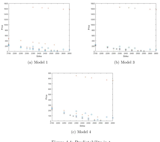
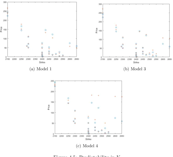
Using the values in Tables A.2, A.4 and A.5, two different figures were generated:
the first stands for the prediction in time to maturity and the second for the
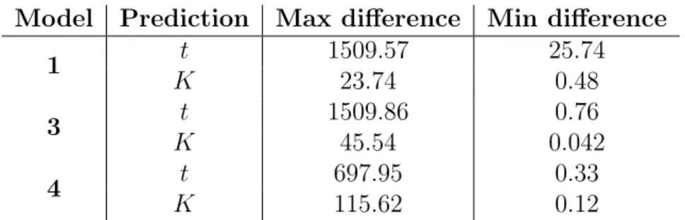
pre-diction in strike. A table was also generated to show the maximum and minimum
differences between real and predicted prices.
Observing Figure 4.4, there is almost no difference between the models. Neither
of the models seems to predict well the prices, particularly for the longest time to
maturity, where the difference is very impressive. This can also be seen on Table
4.3, where we observe that the maximum differences between the real prices and the
predicted ones are 1509.57, 1509.86 and 697.95 for models 1, 3 and 4, respectively.
Looking at Figure 4.5, models 1 and 3 predict the prices in a reasonably way.
Still, these models show some discrepancies between estimated and market prices.
Model 4 predicts the prices worse than the former models, namely for the longer
maturities.
(a) Model 1 (b) Model 3
(c) Model 4
Chapter 4. Results 32
Model Prediction Max difference Min difference
1 t 1509.57 25.74
K 23.74 0.48
3 t 1509.86 0.76
K 45.54 0.042
4 t 697.95 0.33
K 115.62 0.12
Table 4.3: Comparison of prediction ability between models 1, 3 and 4
We can conclude that, although these models estimate the prices much better
than the Black-Scholes model, their prediction ability is not very good. If we wish
to predict the prices with longer times to maturity than those in our sample, they
do not seem to find correct values. The same can be said about the prediction of
prices with strikes outside the sample, even though the results are better in this
Chapter 5
Conclusions
The aim of this dissertation was to improve the famous Black-Scholes model by
letting the volatility of the asset price to be a deterministic function of both time
and asset price and then study the consequences of this change. Choosing the local
volatility to be a parametric function, from a theoretical point of view, does not
introduce many changes: the price of an European vanilla call or put option is still
explained as the solution of a partial differential equation, derived using the same
arguments that Black and Scholes used in their paper. This was possible because
this extended model did not add any new source of uncertainty, unlike stochastic
volatility models or jump diffusion models. The downside was that the solution of
this PDE couldn’t be obtained in a closed form, so we needed to use a numerical
method: the Crank-Nicolson scheme was the selected one.
Four different functions for the local volatility were formulated and all the
pa-rameters involved were calibrated using options on the S&P 500 Index. Numerical
results showed that three of these models performed better than Black-Scholes model
in estimating the option prices, with Model 1 giving the best results. Regarding the
predictive ability, neither of the models performs acceptably in predicting prices
with longer time to maturity than the ones in the sample or with strikes outside
the sample. This is due to the fact that the calibrated parameters show significant
changes from sample to sample.
Bibliography
[1] Black, F. and Scholes, M. (1973). The Pricing of Options and Corporate
Liabil-ities. Journal of Political Economy 81 (3), 637-654.
[2] Hull. J. (2012). Options, Futures and Other Derivatives, 8th ed.
Pear-son/Prentice Hall.
[3] Dupire, B. (1994). Pricing with a Smile, Risk 7 (1), 18-20.
[4] Daglish T., Hull, J. and Suo, W. (2007). Volatility Surfaces: Theory, Rules of
Thumb, and Empirical Evidence.Quantitative Finance 7 (5), 507-524.
[5] Dumas, B., Fleming, J. and Whaley, R. (1998). Implied Volatility Functions:
Empirical Tests, The Journal of Finance 53 (6), 2059-2106.
[6] Brown, G. and Randall, C. (1999). If the skew fits, Risk, 62-65.
[7] Lipton, A. (2002). The vol smile problem.Risk 15, 61-65.
[8] Derman, E. and Kani, I. (1994). The Volatility Smile and Its Implied Tree.
Quantitative Strategies Research Notes, Goldman Sachs.
[9] Coleman, T., Li, Y. and Verma, A. (1999). Reconstructing the Unkown Local
Volatility Function, The Journal of Computacional Finance 2 (3), 77-102.
[10] Merton, R. (1976). Option Pricing when Underlying Stock Returns are
Discon-tinuous. Journal of Financial Economics 3 (1-2), 125-144.
[11] Heston, S. (1993). A Closed-Form Solution for Options with Stochastic
Volatil-ity with Applications to Bond and Currency Options.Review of Financial
Stud-ies 6 (2), 327-343.
Volatilities. The Journal of Finance 42 (2), 281-300.
[13] Achdou, Y. and Pironneau, O. (2005).Computational Methods for Option
Pric-ing. Society for Industrial and Applied Mathematics (SIAM).
[14] Duffy, D. (2006).Finite Difference Methods in financial engineering. John Wiley
& Sons, Ltd.
[15] Duffy, D.Robust and Accurate Finite Difference Methods in Option Pricing One
Factor Models. Available from: http://www.datasimfinancial.com/UserFiles/
articles/daniel3.pdf
[16] Edwards, D. (2015). Numerical and Analytical Methods in Option Pricing.
University of Reading. Available from: https://www.overleaf.com/articles/
numerical-and-analytic-methods-in-option-pricing/rwpzvzwksgrc/viewer.pdf
[17] White, R. (2013). Numerical Solutions to PDEs with
Finan-cial Applications. OpenGamma Quantitative Research. Available
from: https://developers.opengamma.com/quantitative-research/
Numerical-Solutions-to-PDEs-with-Financial-Applications-OpenGamma.pdf
[18] Schoutens, W. (2002).L´evy Processes in Finance. Wiley.
[19] Langtangen, H. (2013). Truncation Error Analysis. Available from: http://
hplgit.github.io/INF5620/doc/pub/main trunc-A4.pdf
[20] Eriksson, A. (2013).A comparison between finite difference and binomial
meth-ods for solving American single-stock options. Master Thesis. Royal Institute of
Technology.
[21] Tavella, D. and Randall, C. (2000). Pricing Financial Instruments: The Finite
Difference Method. John Wiley & Sons, Inc.
[22] Campolieti, G. and Makarov, R. (2014).Financial Mathematics: A
comprehen-sive treatment. Chapman & Hall/CRC.
[23] Rubinstein, M. (1994). Implied Binomial Trees.The Journal of Finance 49 (3),
771-818.
[24] Vidic, I. (2012).Numerical methods for option pricing. Master Thesis.
Politec-nica de Madrid.
[25] Chan, R. (2016).Chapter 9: Numerical Methods for Option Pricing, MAT4210
Notes. Available from: https://www.math.cuhk.edu.hk/course builder/1617/
math4210/ [28 July 2017].
[26] Kuan, C. (2014).Chapter 8: Nonlinear Least Squares Theory, Lectures.
Avail-able from: http://homepage.ntu.edu.tw/∼ckuan/e-courses.html [28 July 2017].
[27] Mukherji, S. (2011). The Capital Asset Pricing Model’s Risk-free Rate. The
International Journal of Business and Finance Research 5 (2), 75-83.
[28] U.S. Department of the Treasury. Available from: https://www.treasury.gov/
resource-center/data-chart-center/interest-rates/Pages/TextView.aspx?data=
billRatesYear&year=2017 [6 July 2017].
[29] MatLab Documentation. Available from: https://www.mathworks.com/help/
curvefit/least-squares-fitting.html [30 March 2017].
Appendix A
Numerical Code, Data and
Parameter Values
A.1
C-N method code
%N - number of time intervals
%M - number of space intervals
%(xmin,xmax) - domain of the space variable
%T - final time
%initial - intial condition: t=0
%down - boundary condition at xmin
%up - boundary condition at xmax
%a,b,c,f - coefficients of the PDE: a*uxx+b*ux+c*u-ut=0 as functions. It
%should be passed as strings: ’a’, ’b’, ’c’ and ’f’ or @a, etc...
function [t,x,u]=CrankN_fit(param,xdata,initial,down,up,a,b,c,f,S0,r)
N=xdata(1);
M=xdata(2);
xmin=xdata(3);
xmax=xdata(4);
T=xdata(5);
%create the grid in time and space