Equity Valuation - Cellnex Telecom S.A.
António Mourato Pereira
Dissertation written under the supervision of Professor José Carlos Tudela Martins
Dissertation submitted in partial fulfilment of requirements for the MSc in Finance, at the Universidade Católica Portuguesa, December 2017
Abstract
Title: Equity Valuation - Cellnex Telecom S.A. Author: António Mourato Pereira
This dissertation presents the valuation of Cellnex Telecom S.A., an independent infrastructure operator for wireless telecommunications traded in the Madrid Stock Exchange. The valuation relies on the application of two models – Adjusted Present Value (APV) and Relative Valuation – followed by a sensitivity analysis with the objective of testing the assumptions made. Through the application of the APV model Cellnex Telecom S.A is valued in €22.81 per share. The Relative Valuation method is only used to better understand how the market currently values similar companies rather than being a support for the investment recommendation. Lastly, this dissertation results are compared and analyzed to the results reported by Morgan Stanley Investment Bank dated 2nd August 2017.
Resumo
Título: Equity Valuation – Cellnex Telecom S.A. Autor: António Mourato Pereira
Esta dissertação apresenta a avaliação da Cellnex Telecom S.A., uma operadora independente de infraestruturas para telecomunicações wireless cotada na Bolsa de Madrid. A avaliação conta com a aplicação de dois modelos – Valor Atual Liquido Ajustado (VALA) e Avaliação Relativa – seguida de uma análise de sensibilidade com o objetivo de testar os pressupostos feitos. Através da aplicação do modelo VALA a Cellnex Telecom S.A é avaliada em €22.81 por ação. O método de Avaliação Relativa é utilizado exclusivamente por forma a melhor perceber como o mercado avalia atualmente empresas similares ao invés de servir de suporte para a recomendação de investimento. Por fim, os resultados desta dissertação são comparados e analisados com os resultados reportados pelo Banco de Investimento Morgan Stanley em 2 de agosto de 2017.
Palavras-Chave: Cellnex, Telecom, Avaliação de Empresas, Valor Atual Liquido Ajustado, Avaliação Relativa
Acknowledgements
First, I would like to express my gratitude to my family for supporting me through my university studies. Secondly, I would like to thank professor José Carlos Tudela Martins for his availability and feedback during the development of this dissertation. And lastly, I would like to thank the valuable inputs both from Cellnex Telecom’s Investor Relations and Ms. Frances from TowerXchange.
List of Abbreviations
TR – Tenancy Ratio
MNO – Mobile Network Operators DAS – Distributed Antenna Systems POP – Point of Presence
TowerCo – Tower Company
CAGR – Compounded Annual Growth Rate EBIT – Earnings Before Interest and Taxes
EBITDA – Earnings Before Interest, Taxes, Depreciation and Amortization CAPEX – Capital Expenditures
D&A – Depreciation and Amortization WC – Working Capital
FCFF – Free Cash Flow to Firm FCFE – Free Cash Flow to Equity APV – Adjusted Present Value ITS – Interest Tax Shields TV – Terminal Value ROA – Return of Assets ROE – Return on Equity
ROIC – Return on Invested Capital EV – Enterprise Value
Index
Introduction ... 8
1. Literature Review ... 9
1.1 Equity Valuation: An introduction ... 9
1.2 Valuation Models ... 10
1.2.1 Discounted Cash Flow Methods ... 10
1.2.1.1 Dividend Discount Model ... 13
1.2.1.2 Free Cash Flow Methods ... 13
1.2.1.3 FCFF - Free Cash Flow to Firm ... 14
1.2.1.4 FCFE - Free Cash Flow to Equity ... 14
1.2.1.5 APV - Adjusted Present Value ... 14
1.2.2 Economic Value Added ... 16
1.2.3 Multiples Valuation ... 16
2 Valuation Model Choice ... 18
3 Industry Overview ... 19
3.1 Telecommunication Services Industry: Overview ... 19
3.2 TowerCo Sector ... 20
4 Cellnex Telecom S.A. ... 22
4.1 Company Overview ... 22 4.2 Business Overview ... 23 4.3 Historical Performance ... 25 5 Company Valuation ... 29 5.1 Forecasting Growth ... 30 5.2 Operational Forecasting ... 31 5.2.1 Revenues ... 31
5.2.2 Operating Expenses and EBITDA Margin ... 32
5.2.3 CAPEX, Depreciations and Amortizations ... 34
5.2.4 Working Capital ... 35
6 APV Valuation ... 37
6.1 Unlevered Cost of Equity ... 37
6.2 Cost of Debt ... 38
6.3 Tax Rate ... 38
6.4 Free Cash Flow to the Firm ... 39
6.5 Debt Plan and Interest Tax Shields ... 39
6.6 Bankruptcy Costs ... 40
6.8 Sensitivity Analysis ... 42
6.8.1 Points of Presence Growth ... 42
6.8.2 Terminal Growth Rate and Unlevered Cost of Equity ... 43
7 Relative Valuation ... 44
8 Investment Recommendation ... 46
9 Investment Bank Report Comparison ... 46
Conclusion ... 48
APPENDIXES ... 50
Introduction
With the purpose of studying different valuation techniques and its practical applications, this dissertation presents a valuation study on Cellnex Telecom S.A. It is structured as follows: First, a Literature Review is presented with the objective of discussing several valuation methodologies, its theoretical foundations and characteristics so that the most suitable method should be chosen. Secondly, and as it is of extreme importance to better understand the company’s dynamics, an analysis is made not only to its Industry but also to its specific Sector and Historical performance. Thirdly, the development of the valuation model as well as the clarification on the assumptions made, a test to those same assumptions and its results. Lastly, the presented results are compared to the ones reported by Morgan Stanley Investment Bank on August 2017.
1. Literature Review
1.1 Equity Valuation: An introduction
Valuation can be described by the process of estimating how much a given asset is worth. This is a central question for many market participants, would they be investors, researchers, business managers, portfolio managers or even regulators. It plays an important role not only in financial markets but also in the financial management of business corporations as it provides valuable insights that support resource allocation which in turn is fundamental for business development and growth. A determining factor in investing activities, valuation is therefore a highly desirable skill, as it contributes for a better decision-making process.
Equity Valuation is the process of estimating how much a given company is worth. According to (Jerald E. Pinto, CFA / Elaine Henry, CFA / Thomas R. Robinson, CFA / John D. Stowe, CFA, 2010) this process can be described as the following steps: understanding the business, forecasting company performance, selecting an adequate valuation model, converting forecasts to a valuation and apply the analytic results in the form of recommendations and conclusions. When valuing an asset, in this case an equity stake, one must take in consideration different definitions of value: Intrinsic Value is the value of an asset assuming a complete understanding of that asset’s investment characteristics - this estimate would reflect the believes of a given investor on which is the ‘true’ value of that asset. On the other hand, Market Value is the value on which the market currently trades an asset reflecting the market believes of its value. According to the Efficient Market Hypothesis the market value of an asset is the best estimate for its intrinsic value. However, assuming the Intrinsic Value can differ from its Market Value constitutes a critical assumption in Equity Valuation, as investment managers constantly seek abnormal returns through mispricing opportunities1. Additionally, there are two assumptions
that are key to company valuation: Going-Concern Value is the value of an asset under the assumption that the company will continue to operate in a foreseeable future; and Liquidation Value is the value of that company’s stock assuming it will be dissolved and their assets will be sold individually, due to being in financial distress2.
The main purpose of Equity Valuation is to apply valuation concepts and models to access a company’s intrinsic value so that a mispricing opportunity can be spotted and exploited. Still,
1 Grossman-Stiglitz Paradox: if all available information is reflected in stock market prices, no agent would have
incentives to acquire information on which prices are based.
2 In some cases, the going concern value might be greater than the liquidation value for companies with constantly
valuation is also useful to: infer market expectations – as market prices reflect investors’ expectations one can ask which expectations lead to the current market price; evaluate corporate events – such as Mergers, Acquisitions, Spin-offs and Leverage Buyouts; appraising private businesses – valuing Initial Public Offerings (IPOs); or even evaluate business strategies – its impact on share value.
1.2 Valuation Models
Deciding on which methods to use will depend on the characteristics of the company being valued, the data available and the questions to be answered. “Although valuation is always a function of three fundamental factors – cash, timing, and risk – each type of problem has structural features that set it apart from the others and present distinct analytical challenges” (Luehrman, Financial Management, 1997)
1.2.1 Discounted Cash Flow Methods
Discounted cash flow methods aim to value a company as the present value of its expected future cash flows discounted at a rate that matches the cash flows’ risk which is represented as the following equation:
𝑉0 = ∑ 𝐶𝐹𝑡 (1 + 𝑟)𝑡 𝑛
𝑡=1
(1)
Discount Rates and Cost of Capital
When valuing a company “analysts need to specify the appropriate rate or rates with which to discount expected future cashflows when using present value models of stock value” (Pinto et al., 2010). These rates reflect investors’ expectations on the return a given investment will generate under the economic principle of opportunity cost. Which is the rate of return required by investors so that they choose to invest in the company rather than investing in a similar project given its riskiness (best available alternative)? Therefore, and alternatively, the discount rate is usually said to be the cost of capital because it represents the rate a company to pays to its investors.
Where,
𝑉0 = 𝑡ℎ𝑒 𝑣𝑎𝑙𝑢𝑒 𝑜𝑓 𝑡ℎ𝑒 𝑎𝑠𝑠𝑒𝑡 𝑎𝑡 𝑡𝑖𝑚𝑒 𝑡 = 0 | 𝑛 = 𝑛𝑢𝑚𝑏𝑒𝑟 𝑜𝑓 𝑐𝑎𝑠ℎ 𝑓𝑙𝑜𝑤𝑠 𝑖𝑛 𝑡ℎ𝑒 𝑙𝑖𝑓𝑒 𝑜𝑓 𝑡ℎ𝑒 𝑎𝑠𝑠𝑒𝑡
Cost of Equity
Cost of equity is the required return of equity investors. The CAPM - Capital Asset Pricing Model3 presents a methodology to access which is the expected return on a given stock, and
therefore, provide an estimate for the cost of equity. The CAPM suggests that a stocks’ return can be described as follows:
𝑅̅̅̅ = 𝑅𝑆 𝑓+ 𝛽 × (𝑅̅̅̅̅ − 𝑅𝑀 𝑓) (2)
where, the expected stock return (𝑅̅̅̅) is equal to the return on a risk-free asset (𝑅𝑆 𝑓) plus a market risk premium (𝑅̅̅̅̅ − 𝑅𝑀 𝑓), adjusted to the stock’s risk relatively to the market (𝛽).
“The attraction of the CAPM is that it offers powerful and intuitively pleasing predictions about how to measure risk and the relation between expected return and risk” (French, 2004). CAPM assumes that investors are risk averse and they make investment decisions based on mean returns and variance of returns of their total portfolios. Although it is the most widely taught and used model, it is important to note that CAPM also entails some drawbacks as it relies on some strong market assumption that might not be realistic (Fernandez, CAPM: an absurd model, 2015).
Beta
Beta (𝛽) is a measure of systematic risk of stock relatively to the market (M). Its calculation results from an ordinary least squares regression of the return on the stock on the return on the market and it is heavily influenced by two factors (Pinto et al., 2010): the index chosen to represent the market portfolio and both the length and frequency of the data used.
It may also be important to make a distinction between levered and unlevered companies to which the Beta will need to be adjusted accordingly. By computing the beta through the previously mentioned method, as we are using market data from publicly traded companies, we will get the levered beta (𝛽𝐿) for the levered cost of equity (𝐾𝑒). Hence,
𝐾𝑒 = 𝑅𝑓+ 𝛽𝐿× 𝑀𝑅𝑃 (3)
On the other hand, if one needs to estimate the Beta for the unlevered company we will need to deleverage the Beta previously computed. According to Hamada (1972), we have the following expression:
𝛽𝐿 = 𝛽𝑈(1 +
𝐷
𝐸(1 − 𝑡)) (4)
“The unlevered beta of a firm is determined by the types of the businesses in which it operates and its operating leverage. Thus, the equity beta of a company is determined both by the riskiness of the business it operates in, as well as the amount of financial leverage risk it has taken on” (Damodaran, 2011).
Therefore, the unlevered cost of equity can be computed as follows: 𝐾𝑢 = 𝑅𝑓+ 𝛽𝑈× 𝑀𝑅𝑃 (5) Market Risk Premium (MRP)
Market risk premium is the incremental premium required by investors relatively to a risk-free asset. Under the CAPM, it is represented by the difference between the expected market portfolio return and the expected return from the risk-free asset adjusted by beta. Although CAPM proved itself a very practical model to estimate market risk premiums, “by the end of the 1980’s, empirical evidence had accumulated that, at least over certain long-time periods, in the U.S. and several other equity markets, investment strategies biased toward small-market capitalization securities and/or value might generate higher returns over the long run that the CAPM predicts” (Pinto, et al., 2010). Eugene Fama and Kenneth French aimed to solve this problem by presenting the 3 factor Fama-French Model that includes: the same factor of the CAPM plus two factors related with company characteristics and valuation – size (SMB) and value (HML). Other approaches might include: historical average, dividend discount model, constant Sharpe ratio method and bond market implied risk premium (Marc Zenner, 2008). Market risk premium is fundamental to estimate capital costs and so, it directly impacts investment decisions. However, as there is not a consensus on which is the best model to estimate MRP and different approaches can lead to different estimates, one should conduct a sensitive analysis in other to evaluate the impact of the different outputs those models can produce.
Cost of Debt (Kd)
Cost of debt represent lender’s required return. Debt Cash Flows, as Pablo Fernandez explains, “are usually riskier than the cash flows promised by the government bonds” and therefore, its required returns will be higher than the risk-free rate.
𝐷𝑒𝑏𝑡 𝑅𝑒𝑞𝑢𝑖𝑟𝑒𝑑 𝑅𝑒𝑡𝑢𝑟𝑛 = 𝐾𝑑 = 𝑅𝐹 + 𝑅𝑃𝑑(𝐷𝑒𝑏𝑡 𝑅𝑖𝑠𝑘 𝑃𝑟𝑒𝑚𝑖𝑢𝑚) (6)
Weighted Average Cost of Capital (WACC)
The WACC is the after-tax weighted average of required rate of return from each capital source (Pinto et al, 2010). This is the most commonly used methodology to access the cost of capital when valuing total firm value through a discount cash flow model. Fernandez (2010) defines WACC as “neither a cost nor a required return, but a weighted average of a cost and a required return”. 𝑊𝐴𝐶𝐶 = 𝑀𝑉𝐷 𝑀𝑉𝐷 + 𝑀𝑉𝐶𝐸𝐾𝑑(1 − 𝑡) + 𝑀𝑉𝐶𝐸 𝑀𝑉𝐷 + 𝑀𝑉𝐶𝐸𝐾𝑒 (7) where, 𝑀𝑉𝐷 = 𝑚𝑎𝑟𝑘𝑒𝑡 𝑣𝑎𝑙𝑢𝑒 𝑜𝑓 𝑑𝑒𝑏𝑡 | 𝑀𝑉𝐶𝐸 𝑖𝑠 𝑡ℎ𝑒 𝑚𝑎𝑟𝑘𝑒𝑡 𝑣𝑎𝑙𝑢𝑒 𝑜𝑓 𝑐𝑜𝑚𝑚𝑜𝑛 𝑒𝑞𝑢𝑖𝑡𝑦 𝐾𝑑 𝑖𝑠 𝑡ℎ𝑒 𝑐𝑜𝑠𝑡 𝑜𝑓 𝑑𝑒𝑏𝑡 | 𝐾𝑒 𝑖𝑠 𝑡ℎ𝑒 𝑐𝑜𝑠𝑡 𝑜𝑓 𝑒𝑞𝑢𝑖𝑡𝑦
As Fernandez (2010) adverts, one should bear in mind that WACC is not a static value but rather a dynamic one. As the company’s capital structure may change overtime, it is important to continuously adjust the WACC calculations for each period. Furthermore, the capital structure, or the Debt to Equity ratio, should be at market values.
1.2.1.1
Dividend Discount Model
The Dividend Discount Model stands one the most basic tools for equity valuation. From the stockholder’s point of view, dividends are the cash flows received in the future plus the market price of the stock in case the shareholder wants to sell it. In turn, the market price will reflect the expected future cash flows – dividends – that given stock will generate afterwards (similar to Terminal Value in Free Cash Flow methods).
For a given finite period n, DDM can be described as follows:
𝑉0 = ∑ 𝐷𝑡 (1 + 𝐾𝑒)𝑡+ 𝑃𝑛 (1 + 𝐾𝑒)𝑛 𝑛 𝑡=1 (8)
1.2.1.2
Free Cash Flow Methods
“The concept of free cash flow responds to the reality that, for a going concern, some of the cash flow from operations is not “free” but rather needs to be committed to reinvestment and
new investment in assets” (Pinto et al., 2010) The two following methodologies, despite their differences, should, theoretically, yield the same results.
1.2.1.3
FCFF - Free Cash Flow to Firm
Free Cash Flow to Firm represents the cash flow available to the company’s capital suppliers after all operational expenses and capital requirements – both CAPEX and Working Capital. Also known as the DCF-WACC method, the FCFF formula will depend on the information available and will reflect the Firm Value of a Company. An example will be as follows:
𝐹𝐶𝐹𝐹 = 𝐸𝐵𝐼𝑇 (1 − 𝑡) + 𝐷&𝐴 − 𝐶𝐴𝑃𝐸𝑋 + ∆𝑊𝐶 (9)
Because FCFF materializes itself as an after-tax cash flow for all capital suppliers its present value is computed using the Weighted Average Cost of Capital.
𝐹𝑖𝑟𝑚 𝑉𝑎𝑙𝑢𝑒 = ∑ 𝐹𝐶𝐹𝐹𝑡
(1 + 𝑊𝐴𝐶𝐶)𝑡 ∞
𝑡−1
(10)
1.2.1.4
FCFE - Free Cash Flow to Equity
Free Cash Flow to Equity represents the cash flow available to common stockholders and can be obtained by deducting the debt holders’ payments to FCFF. Contrary to the FCFF methodology, and given the nature of FCFE, its present value is computed using the risk adjusted rate of return for equity holders – the cost of equity – and will reflect the Equity Value of a Company. 𝐸𝑞𝑢𝑖𝑡𝑦 𝑉𝑎𝑙𝑢𝑒 = ∑ 𝐹𝐶𝐹𝐸𝑡 (1 + 𝐾𝑒)𝑡 ∞ 𝑡=1 (11)
1.2.1.5
APV - Adjusted Present Value
The Adjusted Present Value, firstly introduced by Stewart C. Myers (Myers, 1974), comes as an alternative to the traditional use of DCF-WACC method based on the previous work developed by Modigliani and Miller (Miller, 1958). This model allows not only to analyze how much a given asset is worth but also to evaluate where value is generated since it separate each component of value and analyze them separately. These two models differ mainly on “how they account for the value created or destroyed by financial maneuvers” (Luehrman, Financial Management, 1997).
Adjusted Present Value begins with the same methodology as the other discounted cash flow models. First, one needs to forecast future cashflows and access a suitable terminal value and
discount those at a discount rate in line with the riskiness of the cash flows. We will do this assuming the company is totally equity financed and so discounting at the cost of equity for the unlevered company – unlevered cost of equity (Fernandez, 2004). Secondly, we will add up our valuation of the financing side effects, such as: interest tax shields, the costs of issuing new securities, the costs of financial distress and subsidies to debt financing (Stephen A. Ross, 2013).
𝐴𝑃𝑉 = 𝑃𝑉(𝑈𝑛𝑙𝑒𝑣𝑒𝑟𝑒𝑑 𝐹𝑖𝑟𝑚) + 𝑃𝑉(𝐹𝑖𝑛𝑎𝑛𝑐𝑖𝑛𝑔 𝑠𝑖𝑑𝑒 𝑒𝑓𝑓𝑒𝑐𝑡𝑠) (12) Interest Tax Shields
Interest Tax Shields are a result of the “deductibility of interest payments on the corporate tax return (…) the interest deduction will reduce taxable income by the amount of the interest and so will reduce the tax bill by the amount of interest times the tax rate” (Luehrman, Financial Management, 1997)The latter statement holds true if all interest paid is tax-deductible (Fernandez, 2004). Although the Value of Tax Shields (VTS) is one of the main concerns in this type of valuation, there is not a consensus on which is the best methodology to compute its present value. According to Meyers (1974), we should compute the present value of the tax shields at the cost of debt, assuming the riskiness of the tax payments is the same as from its underlying debt.
Bankruptcy Costs
Capturing tax reductions through increasing the level of debt can be tempting. As “Modigliani and Miller argue that the firm’s value rises with leverage in the presence of corporate taxes” (Stephen A. Ross, 2013) due to the VTS. Nevertheless, we should bear in mind that increasing debt levels also brings some costs – namely, Financial Distress Costs. An optimal amount of debt derives from offsetting the up effects of tax shields with the down effects of financial distress costs.
Terminal Value
Free Cash Flow Discount models consist on computing the present value of forecasted future cash flows. However, as we cannot estimate cash flows forever, one should estimate cash flows for the growth period and then, when growth is stable, a Terminal Value which represents all cash flows generated thereafter. According to Ross et al., (2013) Terminal Value is estimated by assuming a constant perpetual growth rate for cash flows beyond the horizon, T, so that:
𝑇𝑉𝑇 =𝐶𝐹𝑇(1 + 𝑔𝐶𝐹)
𝑅𝑊𝐴𝐶𝐶− 𝑔𝐶𝐹 (13)
Computing the Terminal Value is of extreme importance as it carries great value for the valuation itself. Hence, an analyst should be careful because “any analysis is as accurate as the forecasts it relies on” (Tim Koller, 2010). The Free Cash Flow Methods previously presented, specifically expressing the Terminal Value are as follows:
𝐹𝑖𝑟𝑚 𝑉𝑎𝑙𝑢𝑒 = ∑ 𝐹𝐶𝐹𝐹𝑡 (1 + 𝑊𝐴𝐶𝐶)𝑡+ 𝑇𝑒𝑟𝑚𝑖𝑛𝑎𝑙 𝑉𝑎𝑙𝑢𝑒 (1 + 𝑊𝐴𝐶𝐶)𝑡 𝑛 𝑡−1 (14) 𝐸𝑞𝑢𝑖𝑡𝑦 𝑉𝑎𝑙𝑢𝑒 = ∑ 𝐹𝐶𝐹𝐸𝑡 (1 + 𝐾𝑒)𝑡+ 𝑇𝑒𝑟𝑚𝑖𝑛𝑎𝑙 𝑉𝑎𝑙𝑢𝑒 (1 + 𝐾𝑒)𝑡 𝑛 𝑡=1 (15)
1.2.2 Economic Value Added
Economic Value Added (EVA) is one of the applications of the residual income concept and aims to capture how much value is being created (destroyed). Residual income is considered to be the remaining income after deducting all costs related to the company’s capital (Pinto, et al., 2010). Thus, EVA is the Net Operating Profit after Taxes (NOPAT) less total capital costs and may be represented as follows (Fernandez, Three Residual Income Valuation Methods and Discounted Cash Flow Valuation, 2015):
𝐸𝑉𝐴𝑡= 𝑁𝑂𝑃𝐴𝑇𝑡− (𝐷𝑡−1+ 𝐸𝑏𝑣𝑡−1)𝑊𝐴𝐶𝐶 (16)
Fernandez, 2002 makes a note that the above described formula mixes accounting parameters (NOPAT, Debt and Equity at book value) with market parameters (WACC) which raises the need to some adjustments to be made (Pinto et al., 2010).
Related with the EVA concept is the Market Value Added (MVA) that results from the difference between the market value of a company and its book value. Fernandez, 2002 identifies MVA as the present value of the EVA discounted at the WACC. Hence:
𝑀𝑉𝐴0 = [𝐸0+ 𝐷0] − [𝐸𝑏𝑣0 + 𝐷0] = 𝑃𝑉(𝑊𝐴𝐶𝐶; 𝐸𝑉𝐴) (17)
1.2.3 Multiples Valuation
Multiple valuation is still one of the most used techniques in equity valuation. Despite DCF-based methods being the most accurate and flexible methods, Multiples Valuation are a useful,
practical and easy to use tool to confirm valuation results reflecting the “current mood of the market” (Damodaran). Generally, “a multiple summarizes in a single number the relationship between the market value of a company’s stock (or of its total capital) and some fundamental quantity, such as earnings, sales or book value” (Pinto et al., 2010).
There are two main methods in multiples valuation: the method of comparables which refers to valuing an asset based on multiples of similar assets; and the method of forecasted multiples which bases itself on forecasted fundamentals. In the case of comparables method, the notion of similar assets is critical because by similar firms we should understand the ones that “have the same operating and financial characteristics as the firm being valued” (Schreiner, 2007). Therefore, to conduct the valuation we first must select a peer group - a small group of companies that have identical growth, performance and risk profiles – understand why they have those multiples and then explore the differences. According to Koller, et al. (2010) one should select the peer group based on companies whose underlying characteristics lead to similar Return on Invested Capital (ROIC) and long-term growth.
There is a wide range of multiples based on capitalization, on company’s value and even on growth. Nevertheless, Fernandez (2017) shows that the most commonly used multiples by analysts for valuing European companies are P/E and EV/EBITDA. According to Koller et al., (2010) one should always start with EV/EBITDA because “it tells more about a company’s value than any other model”.
If in one hand, multiples approach presents several benefits by its simplicity, practicality and availability, on the other hand these same benefits represent also a weakness. According to Damodaran (2011) they can lead to inconsistent estimates of value due to: incorrect selection of a peer group; market over or under valuation; lack of transparency regarding the underlying assumptions.
Enterprise Value / EBITDA
EV/EBITDA is a valuation indicator for the overall company. Koller et al., (2010) state that there are four factors that drive EV/EBITDA multiple: the operating tax rate, the cost of capital, the company’s growth rate and its ROIC – Return on Invested Capital:
𝐸𝑉 𝐸𝐵𝐼𝑇𝐷𝐴=
(1 − 𝑡)(1 −𝑅𝑂𝐼𝐶)𝑔
There are several other Enterprise Value Multiples that can be used depending on the analyst preferences such as: EV/Sales, EV/Book Value, EV/EBITDA Growth. The main argument for using EV multiples rather than Price multiples is that EV multiples are relatively less sensitive to the effects of financial leverage (Pinto et al., 2010).
Price to Earnings
Price/Earnings is the most used multiple in equity valuation from a wide range of other price multiples that might include: P/CE – Price to cash earnings, P/S – Price to sales and P/BV – Price to book value.
𝑃𝑟𝑖𝑐𝑒 𝑡𝑜 𝐸𝑎𝑟𝑛𝑖𝑛𝑔𝑠 =𝑃𝑟𝑖𝑐𝑒
𝐸𝑃𝑆 (19)
Despite being extremely used, P/E also has some significant drawbacks mainly deriving from EPS characteristics. First, P/E has no meaning in a scenario with negative or low net income and secondly, EPS relies on accounting rules which can present some interpretation issues.
2 Valuation Model Choice
Cellnex’s current strategy aims towards an European expansion of their business which will require heavy capital investments that have been financed mostly by issuing debt. Since higher levels of capital might be needed to fund growth and given the fact that there are no guidelines for capital structure, the only thing we can expect is that capital structure will face some changes in the future. Therefore, and with a changing capital structure the model of choice is the Adjusted Present Value. Moreover, we believe that a detailed analysis to value creation and its origins assumes a major importance in Cellnex’s context.
Additionally, a valuation based on multiples – Relative Valuation – will be performed so that we can value Cellnex with a different perspective. This will allow us to better understand how the market values similar companies and to what extent it differs to the results given by the APV Model.
3 Industry Overview
3.1 Telecommunication Services Industry: Overview
“Greater speed, flexibility and a willingness to collaborate are critical – both for creating new revenue opportunities as well as reducing risk and operating expense – if providers are to maintain their industry leadership.” – IBM
Telecommunication Services Industry comprehends companies operating wireless and/or fixed-line telecommunication networks for voice, data and high-density data. Telecommunication is any communication over a distance, would it be via telephone, radio, television, wireless network or computer network. Telecom Industry companies build, maintain and operate telecommunication networks that enable one of the most important services to modern society: the ability to communicate intra and cross borders.
The Telecom Industry is highly dependable of technological advancements since those are the catalysts for the creation of new products and processes that affect the entire value chain. If at one time, there was the need for physical wires to exist connecting homes and businesses so that communication at distance would be possible, today, we live in a society of wireless technology, connecting people and moving data all over the world in seconds. As digital technology evolved, new technologies have been shaping the Telecom Industry and Mobile has
been the key driver of these transformational process.
Moreover, 3G technology4, for example, was a breakthrough technology in communications as
it allowed faster communication services from voice to messaging and webservice. The introduction of internet-based communication services has been shifting away value from the
4 3G Technology is the third generation of wireless technology. It provides faster communication services than
previous technologies, including voice, messaging and web services anytime anywhere with a seamless global roaming. Today, Telecom companies are already investing to prepare themselves for the roll-out of 5G technology (2020, expected) Find more about Mobile Wireless Technologies in the Appendix 1
0 2 4 6 8 10 2010 2012 2014 2016 2018 2020 M obi le C on ne cti on s in B illi on s
traditional communication services requiring Telecom Companies to adapt their business models to stay competitive in the market5.
Today, to keep up with new technologies, Telecom Companies face high capital investments both for the development of their core products and services and the infrastructure that supports those same products and services. Telecom companies can own, operate and maintain these infrastructure assets by themselves or, as usually happens, they can establish alliances with other Telecom operators to collectively manage those assets and share its costs. As an alternative, it has been frequent to Telecom Operators to sell their network infrastructures to independent infrastructure operators and lease them back – Sell-to-Leaseback strategy. This strategy not only allows Telecom Operators to free-up cash that may be used to product development but also gives them access to the best practices on network management and, therefore, a network that is continuously being improved and up-to-date with recent technologies6.
3.2 TowerCo Sector
Given the developments of the Telecommunications Industry, the TowerCo sector – “wholesale infrastructure providers” – have been experiencing an expansion in terms of towers under management. Although communication towers have been acquired by TowerCos for quite some time in the United States and India, European TowerCos have been growing substantially mainly over the last decade.
5 EY ‘Changing ecosystem dynamics – past, present and future’ – Appendix 2 6 Pros and cons sell to leaseback – Appendix 3
100% 68% 82% 36% 0% 20% 40% 60% 80% 100%
China India USA Europe
In early 2016, approx. 36% of the total towers in Europe were owned and managed by TowerCos whereas in United States the proportion of independently owned towers were nearly 82%. Therefore, there is still room for growth in the European Market.
China is the only continent were all towers are independently owned, being China Tower Company the world’s largest TowerCo with 1 160 000 towers under management. In the second place comes Indus Towers (India) with 117 579 towers under management followed by American Tower with 99 600 towers worldwide. Deutsche Funkturm, from Deutsche Telecom, is the largest European TowerCo with 27 000 towers under management7.
TowerCos, as independent infrastructure providers, are responsible for investing in the development and maintenance of their own tower networks. Since they are specialized in Telecom Infrastructure it becomes easier to work towards an efficient network: increasing the number of network operators per tower and improving coverage in areas where it was not profitable for network operators to invest in additional infrastructure (e.g. Rural areas).
There are two main drivers for growth in the Tower Infrastructure Market:
Coverage Obligations: Usually imposed by country’s telecommunication regulators, population coverage or network investment obligations are related to the allocation of frequencies requiring operators to provide certain degree of coverage until a pre-defined date.
Mobile Data Traffic Growth8: In Europe, mobile data traffic is expected to grow at a
Compounded Annual Growth Rate (CAGR) of 42% from 2016 to 2021. The increasing popularity of mobile devices and applications as lead to a greater demand for mobile bandwidth supporting the exponential growth of data usage. As a result, MNOs focus on competing on network quality to which will rely even more on specialized infrastructure services.
In both cases, as operators need to increase coverage or network data capacity, spectrum9 limitations might apply. Therefore, tower rental is an efficient solution for
both cases since they can use a third-party infrastructure to increase their network.
7 Please find additional data on the European Tower Market in Appendix 4 8 Mobile Data Traffic Growth CISCO VNI - Appendix 5
4 Cellnex Telecom S.A.
4.1 Company Overview
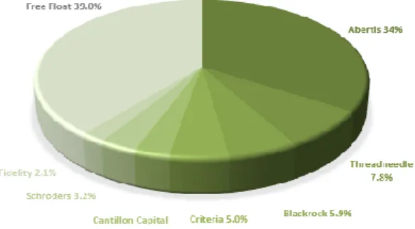
Cellnex Telecom is the main independent infrastructure operator for wireless telecommunication in Europe currently operating a network of more than 24 000 sites and providing services to network operators across Spain, Italy, Netherlands, France, United Kingdom and Switzerland. Formerly known as ‘Abertis Telecom’, Cellnex is listed in the continuous market of the Spanish Stock Exchange and is part not only of the selective IBEX 35 and EuroStoxx 600 Indices but also of the FTSE4Good Sustainability and Carbon Disclosure Project (CDP) indices. Its IPO is dated the 1st of April 2015 as a result of a spin-off from
ABERTIS Group – which still holds a 34% equity stake in the company. Company Ownership
Share Price
Graph 1 – Cellnex Share Price. Source: Thomson Reuters
31/10/2017; €21,315 10,00 € 12,50 € 15,00 € 17,50 € 20,00 € 22,50 € 25,00 €
4.2 Business Overview
Cellnex’s business model is based on the provision and sharing of telecommunications assets, acting as an independent and neutral infrastructure provider for telecommunication operators10.
Cellnex offers its customers the space they need to install and maintain their communications network equipment and provide wireless voice and data transmission. Additionally, it also provides ‘the most advances audiovisual services to national, regional and local broadcasters’. Products and Services
Cellnex provides services related to infrastructure management for terrestrial telecommunications divided in three main segments:
Telecom Infrastructure Services: providing the access to broadcasting and communication sites to Mobile Network Operators (MNOs) and other broadband and wireless telecom network operators through site hosting and co-location of telecommunication equipment.
Broadcasting Infrastructure: it consists in the network operation and radio-electric spectrum management to ensure distribution and broadcasting of digital television, radio or multi-screen environment content.
Other network services: it includes other connectivity services to telecom operators, Public Protection and Disaster Relief (PPDR) services, operations and maintenance services, urban telecom infrastructure, and others.
10 Tower Business Overview – Appendix 7
21% 46% 52% 61% 39% 35% 19% 15% 13% 2014 2015 2016
Telecom Infrastructure Services Broadcasting Infrastructure Other Network Services
Strategy
Since its IPO, Cellnex main strategy is the European expansion and consolidation focusing on the Telecom Infrastructure Services segment. They have been doing so primarily through M&A (inorganic) growth in a three-stage process: the first step is - Introduction - in a given country which allows to get a direct relationship with the costumers and identify new opportunities for growth; the second step is – Scale - aiming to growth the business in that country to gain a critical dimension and market position; and the third step is – Consolidation - where it is important to have a nationwide footprint to consolidate and further develop partnerships and cooperation programs with clients. Besides Telecom Infrastructure Services being the main focus for M&A growth, Cellnex might also consider this strategy to expand its Broadcasting Infrastructure if: it allows them to consolidate a leading position in a country other than Spain, or; if the relevant assets are part of a portfolio of sites similar to their portfolio.
Telecom Infrastructure Services organic growth is based on three distinct pillars:
Multi-Tenancy: by increasing the number of tenants in each tower site and therefore expanding the provision of site rental services to telecom operators, Cellnex is able to leverage their extensive existing tower infrastructure capitalizing on the growth in the number of PoP in their markets.
Rationalization: through the acquisition of tower sites from several carriers, Cellnex is able to rationalize the network by decommissioning redundant towers resulting on a single efficient network used by several carriers.
Built-to-suit: Cellnex aims to construct build-to-suit towers for telecom operators in certain instances as a way to increase their potential to capture future growth in co-location demand.
As for the Broadcasting Infrastructure segment, Cellnex priority is to maintain a leading position in the national digital TV sector and increase their market share in the regional and local TV and radio broadcasting markets by leveraging their know-how on the tower and network infrastructure market. According to Cellnex, Broadcasting Infrastructure shows significant revenue visibility since revenues are generated based on the number of signal transmitted rather than on the number of users that receive or see the signals. Therefore, it has proven itself resilient towards economic cycles and macro-economic downturns.
Regarding their third business segment, Network Services & Other, Cellnex aims to capture growth by: expanding and increasing data transmission connectivity services; leveraging their infrastructure and frequency planning know-how to design, roll-out and operate advanced telecom services for public administrations in the field of PPDR networks; developing urban telecom infrastructure solutions and small-cells; continuing to provide O&M services to telecom companies.
4.3 Historical Performance
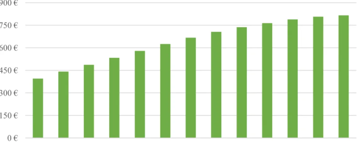
RevenuesFrom 2011 to 2013 Cellnex revenues were growing at a -3% per year leading to approx. €385Mn in 2013. In 2014 revenues registered a growth of 13% resulting from an additional effort to boost revenues reinforcing the current business segments essentially through new leases to MNOs. After starting preparing it in 2014, 2015 was the IPO year with new sources of financing boosting the expansion to new geographies. To date, the biggest annual growth in revenues was in 2015 registering a rate of 40%. In 2016, revenues growth slowed down to 15% reaching approx. €700Mn.
Figure 5 – Total Revenues in € Millions. Source: Cellnex Telecom S.A. EBITDA and EBITDA Margin
In the previous graph, one can see both the evolution of Earnings Before Interest, Taxes, Depreciation and Amortization in gross value and in percentage of revenues – which stands as EBITDA Margin. Although it is possible to identify some positive correlation between the value of EBITDA and corresponding EBITDA Margin from 2011 to 2013 this is not true for the years of 2014 and 2015. In fact, besides EBITDA has been growing since 2013, EBIDTA margin does not follow the same trend. The reason behind this behavior relies on the fact that operational costs have been growing at a higher rate than revenues for the years of 2014 and
300 € 400 € 500 € 600 € 700 € 800 € 2011 2012 2013 2014 2015 2016
2015 mainly due to the increase of operational costs relating to the IPO process that were recognized on those periods. 2016 already registered a slight increase on EBITDA Margin, to 39%.
Figure 6 – EBITDA (€ Millions) and EBITA Margin (%). Source: Cellnex Telecom S.A. Operating Profit, Earnings Before Tax and Net Profit
In the graph below, it is possible to see the relation between Operating Profit, Operating Profit after Net Financial Costs and Operating Profit after Net Financial Costs and Taxes (Consolidated Net profit). From 2014 onwards, it becomes clear the effect of the increase in the debt level, leading to the increase of financial costs. Additionally, it is also interesting to see that in the year of 2015 a significant stake of the results for the period – Consolidated Net Profit – were possible due to tax policies. In the year of 2016 it is also possible to identify a favorable tax policy has the effective tax rate was 1.5%.
Figure 7 – EBIT, Earnings Before Tax and Consolidated Net Profit in €Millions
0% 20% 40% 60% 80% 100% 0 € 50 € 100 € 150 € 200 € 250 € 300 € 2011 2012 2013 2014 2015 2016
EBITDA EBITDA Margin
0 € 20 € 40 € 60 € 80 € 100 € 120 € 2011 2012 2013 2014 2015 2016
Capital Expenditures and Depreciation and Amortization
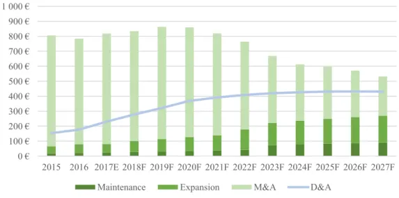
In terms of Capital Expenditures, and for the years prior the IPO, these amounts were mainly due to the investment in existing assets. From 2014 onwards, the expansion strategy lead to higher levels of M&A activity requiring higher levels of Capital to fund the acquisition of new assets. Therefore, and as the asset base increased significantly during 2014-2016, we can also see a significant rise on the level of Depreciation and Amortizations.
Figure 8 – CAPEX, Depreciations and Amortization in €Millions Total Debt and Net Debt
Below, we can see the company’s Total Debt and Net Debt from 2011 to 2016. The access to the markets allowed Cellnex to capture the funding they needed to expand. Total debt in 2016 represents 10.6x the debt level in 2013 and 3.9x the debt level in 2014. One may also notice that the level of cash the company holds is also higher as they need to be prepared to meet their current obligations.
Figure 9 – Debt and Total Debt in €Millions
0 € 200 € 400 € 600 € 800 € 1 000 € 2011 2012 2013 2014 2015 2016 CAPEX D&A 0 € 250 € 500 € 750 € 1 000 € 1 250 € 1 500 € 1 750 € 2 000 € 2011 2012 2013 2014 2015 2016
Working Capital
From 2011 to 2016, Working Capital has registered some significant changes being ‘Trade and other receivables’ and ‘Other current assets and liabilities’ the accounts that have changed more expressively. As reported, Inventories represent a small portion of Working Capital as it comprehends mainly technical equipment which, after installation, will be sold.
Figure 10 – Working Capital in €Millions
-80 € -60 € -40 € -20 € 0 € 20 € 40 € 60 € 2011 2012 2013 2014 2015 2016
Changes in current assets/current liabilities Inventories
5 Company Valuation
This section presents the valuation of Cellnex Telecom S.A.. As explained in Section 2, an Adjusted Present Value approach will be used to conduct the valuation followed by a sensitivity analysis to test the impact of a change on key valuation metrics. Additionally, the APV valuation results will be compared with the ones resulting from a Relative Valuation based on Multiples so that we can access how the market values similar companies.
The next sections will explain the details and assumptions made regarding the forecasting exercise needed for the APV model and the assumptions on the model itself.
The currency of this valuation is Euros (€). Explicit period
We will assume an explicit period of 10 years going from 31st Dec 2017 to 31st Dec 2027. The
explicit period translates what we will generally define as 3 different phases:
• A first phase where M&A Growth will be more evident. This phase identifies a period during which the M&A activity is believed to be more intense following recent growth [2017-2020]
• A second phase where M&A Growth will be gradually slowing down as Cellnex focus is assumed to be the consolidation of its business, essentially through network efficiencies. Growth is also expected to be originated from DAS Nodes projects both in term of existing networks and additional projects (e.g. IoT and Public networks). [2020-2026]
• And lastly, a third phase, were Cellnex is believed to become stable. [2027+] Terminal Growth Rate
When analyzing growth, and giving Cellnex’s current strategy, it is clear to see that there are some limits to growth as there might be a limited amount of tower portfolios to be acquired in Europe. Although it is mentioned that DAS Nodes are the future growth driver for Telecom Infrastructure Services there is still some uncertainty regarding quantifying its effects.
In valuation, it is common to assume as Terminal Growth Rate a proxy for the long-term economy growth usually estimated to be around 2%. Nevertheless, we will take a more conservative approach on long term growth accounting for the existing uncertainties and assuming a Terminal Growth Rate of 1%.
5.1 Forecasting Growth
As previously explained, Cellnex business highly relies on its infrastructure. Therefore, the first step into the forecasting exercise consists in accessing future infrastructure growth based on company guidelines and market expectations. In this valuation, we will forecast infrastructure based on Points of Presence [PoPs] which will be a valuable input to our model.
Overall it is forecasted that the total number of Cellnex’s new PoPs will grow at a CAGR of 10.4% from 2017 to 2027, accounting for 78 750 PoPs in 2027. We forecasted both Organic and M&A growth new PoPs taking in account the following guidelines11:
Organic Growth: Cellnex presents a guidance of 3-4% organic growth guideline until 2019 and this is assumed to be a reasonable guideline for years to come. The nature of organic growth, however, may vary throughout the explicit period. If, to date, organic growth has been greatly influenced by consolidation and improvements on network infrastructure boosted by M&A activity, those effects are expected to decrease through the explicit period. Nevertheless, we also believe that the possible down effects of M&A activity on Organic New PoPs will be overcome by the positive effects of increasing new DAS Nodes projects, keeping organic growth within the mentioned guidelines. M&A Growth: Cellnex does not present a guideline for M&A new PoPs since it depends on Cellnex’s investment opportunities throughout the years and the quality of the portfolios acquired. Besides being hard to accurately forecast M&A Growth, it is also very important to include it in the valuation since it has been and will be a key driver of growth. As a way of overcoming this challenge and so that the forecasted numbers were realistic, some research was made regarding the current state of the European Market, its development in recent years and the current expectations and forecasts regarding the market as a hole for years to come.
One of the most important sources of information was TowerXchange, a leading research institution on Tower Markets worldwide. According to TowerXchange12, at
year end 2020, 44% of the total 600 000 European tower structures will be owned by independent TowerCos. If we assume that Cellnex maintains its current market share of 22.2% – Cellnex at year end 2016 owns 16 828 towers versus European total of 75 867 towers reported by TowerXchange – it implies that Cellnex will own 59 067 towers in
11 Please see detailed information regarding growth forecast in Appendix 12 – Base Case 12 TowerXchange Europe Dossier 2017
2020. Additionally, if we assume a Tenancy Ratio of 1.65, which is considered to be a near efficient market tenancy ratio according to Analysys Mason13, it gives us
approximately 97 460 PoPs.
When analyzing these results, and taking in account both the recent nature of Cellnex Telecom and the overall state of the market, we found that this growth might be a little overestimated. In fact, TowerXchange lowered their forecasts from 2016 to 2017 in about 8% and agreed that, in reality, this growth might take longer to materialize. Therefore, their forecasts and the above described rationale were used just as a reference to estimate M&A Growth – we assumed that the forecasted values for 2020 are an approximation for the European market structure in a mature stage – which according to our model occurs only in the 2027 horizon.
Table 1 – Forecasted Number of Points of Presence (PoPs). Source: Cellnex Telecom S.A. | Own Calculations
5.2 Operational Forecasting
5.2.1 Revenues
Telecom Infrastructure Services
The Telecom Infrastructure Services revenues are estimated based on the forecasted number of Points of Presence for each period and the Revenue per PoP registered in 2016 aiming to reflect the most recent pricing practice. As revenues are based on long-term contracts, the price per PoP is not expected to change significantly over the explicit period. Other operating income and advances to costumers are defined as a percentage of revenues based on the average weight it represented for the years of 2015 and 2016.
Broadcasting Infrastructure
The Broadcasting Infrastructure segment is concentrated in the Spanish market and there are no expectations to Cellnex to expand this activity to other markets any time soon. Hence, and given the stable outlook for the Spanish Broadcasting market, revenues are forecasted as a moving average for the last two periods resulting in a stable revenue generation.
Other Network Services
Other Network Services are expected to follow the same trend as Telecom Infrastructure Services segment since they are greatly related to that activity. Therefore, Other Network Services are forecasted as a percentage of total revenues based on its average weight in 2015 and 2016.
Figure 11 – Revenues per Segment in €Millions. Source: Cellnex Telecom S.A | Own Calculations
5.2.2 Operating Expenses and EBITDA Margin
As reported, Operating Expenses14 are divided into four major categories: Staff Costs, Other
operating expenses, Change in provisions and Losses on fixed assets. The latter two were kept constant for simplicity. The forecasting of Staff Costs was based on an estimate of the number of Staff (Cellnex Group) for each year times the average Cost/Staff registered in 2015 and 2016. At year end 2016, and as a comparison to 2015, the staff balance increased by 58 employees both as a result of regular recruitment needs and incorporation of new businesses into the group.
14 Please see detailed information in Income Statement – Appendix 14
0 € 250 € 500 € 750 € 1 000 € 1 250 € 1 500 € 1 750 € 2 000 € 2015 2016 2017E 2018F 2019F 2020F 2021F 2022F 2023F 2024F 2025F 2026F 2027F Tel. Inf. Ser. Broad. Ser. Other Net. Ser.
Therefore, and as an approximation, it was assumed that this staff balance would register an increase of 50 employees per year.
Other operating expenses include Repairs and Maintenance, Leases and Fees, Utilities and Other Operating Costs and are forecasted as a percentage over revenues. Cellnex mentions that, if wasn’t for the effects of M&A activity, these operating expenses would have remained relatively flat over the last years. Furthermore, significant operational efficiencies have been reached regarding energy, optimization of ground leases and network re-designing leading to an overall reduction of its weight relatively to revenues of 1.4%. Hence, and assuming that Cellnex Telecom S.A. will have capacity to further present operational cost reductions, we assume a yearly decrease of 1% it the weight of Other Operating Expenses over total Revenues.
Figure 12 – Operating Expenses in €Millions. Source: Cellnex Telecom S.A | Own Calculations
Due to the before mentioned growth both in terms of revenues and operational costs, EBITDA shows itself gradually increasing, going from 40.0% in 2017 to 54.7% in 2027. In historical terms, as described in previous sections, Cellnex’s EBITDA Margin was about 38%. After registering an EBITDA margin of 37% in 2016, our forecasts imply that Cellnex will be able to increase its operational efficiency in a very significant way. Many times, and as it will be discussed later on this dissertation, American Tower Companies are seen as the role model for European Tower Companies. If we consider that American companies currently have EBITDA Margins of nearly 60%, we can see that Cellnex’s EBITDA Margin actually goes in accordance with its American Peers15.
15 Please find additional data on Appendix 13 regarding American Peers
0 € 150 € 300 € 450 € 600 € 750 € 900 € 2015 2016 2017E 2018F 2019F 2020F 2021F 2022F 2023F 2024F 2025F 2026F 2027F Operating Expenses
Table 2 – EBITDA Margin. Source: Own Calculations
5.2.3 CAPEX, Depreciations and Amortizations
Total capital expenditures (Capex) comprehends: Maintenance Capex - investment in existing tangible or intangible assets, such as investment in infrastructure, equipment and information technology systems, and are primarily linked to keeping sites in good working order, but which excludes investment in increasing the capacity of sites; Expansion Capex - Investment to the network of tower infrastructures, equipment for radio broadcasting, network services, cash advances, land acquisitions and others that generate additional adjusted EBITDA; M&A Capex - Investments in shareholdings of companies as well as significant investments in acquiring portfolios of sites (asset purchases).
Besides not being a consensual methodology between practitioners, in this valuation we will consider M&A investments as Capital Expenditures. Following Damodaran’s perspective, if one accounts for M&A effects on company growth – as we did in this valuation – one should also account for its costs.
Maintenance Capex will be forecasted based on company guidelines – 3% of revenues. However, from 2023 onwards, we consider that maintenance capex will be 5% of revenues aiming to reflect the need of additional investments to maintain their assets both due to the greater dimension of the portfolio and the new assets related to DAS Nodes projects.
Expansion Capex will also be within the company guidelines of 5-10% of total revenues. From 2022 onwards, and again, we assume that it represents 10% of revenues aiming to reflect the additional investments related to the development of DAS Nodes projects. M&A Capex will be forecasted based on the M&A PoPs for each period and an historical Capex/PoP estimate. However, for the year of 2017, we considered the CAPEX/PoP announced in their latest results presentation so that a more realistic estimate would be made. For all the other periods, the CAPEX/PoP input was based on the corresponding average for the years 2015, 2016 and 2017E.
Once total investment is calculated, we proceed to the corresponding adjustments to tangible and intangible assets to estimate the corresponding depreciation/amortization and resulting
carrying amounts. For each year, we forecasted not only the effects of additions (Capex) in tangible and intangible assets but also the effects from the incorporation of new assets (“Changes in consolidation scope”), based on an asset contribution per forecasted M&A PoPs following the same rationale as other estimates in this dissertation.
As it is common to happen in recent companies with the objective of deferring tax payments in their prior years, Cellnex Telecom mentions that they recur to accelerated depreciation/amortization methods. Since higher rates are used in prior years, there is the need for some adjustments regarding the subsequent periods. From 2017 to 2019, as the M&A PoPs acquired continue to grow, we assumed the same depreciation rates as observed in 2015 and 2016. From 2019 onwards, we estimated a reduction of 6% per year16 in the annual
depreciation/amortization rate translating the before mentioned adjustments.
Figure 13 – CAPEX, Depreciations and Amortizations in €Millions. Source: Cellnex Telecom S.A. | Own Calculations
5.2.4 Working Capital
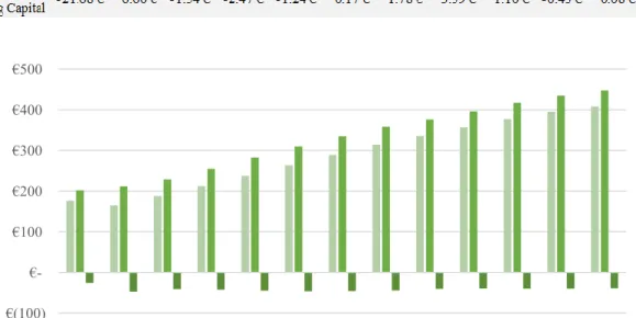
Working Capital is estimated as the difference between non-cash current assets and non-debt current liabilities including current deferred tax assets and liabilities as it is believed that deferred taxes will be continuing to be present and influence short term operations. All accounts are estimated as a percentage of total revenues based on the corresponding 2016 weights with the exception of deferred taxes that were treated separately. Deferred tax assets were forecasted using a moving average and assuming that they will be fairly constant throughout the explicit
16 Based on the reported deferred tax liabilities arising from accelerated depreciation and amortization and
assuming a tax rate of 25% (Spanish Corporate Tax Rate) we estimated what would be the “real” rate for the years of 2015 and 2016. The 6% reduction rate aims to bring the depreciation/amortization rates in year 2027 to the estimated “real” rates.
0 € 100 € 200 € 300 € 400 € 500 € 600 € 700 € 800 € 900 € 1 000 € 2015 2016 2017E 2018F 2019F 2020F 2021F 2022F 2023F 2024F 2025F 2026F 2027F Maintenance Expansion M&A D&A
period whereas the deferred tax liabilities are expected to decrease especially due to the slowdown of M&A activity.
Table 3 – Changes in Working Capital in €Millions. Source: Own Calculations
Figure 14 – Working Capital Dynamics in €Millions. Source: Own Calculations
€(100) €-€100 €200 €300 €400 €500 2015 2016 2017E 2018F 2019F 2020F 2021F 2022F 2023F 2024F 2025F 2026F 2027F Non-Cash Current Assets Non-Debt Current Liabilities Working Capital
6 APV Valuation
This section will introduce the application of the Adjusted Present Value methodology to value Cellnex Telecom. As discussed before, the APV approach starts by evaluating the company as if it was all equity financed and then accounts for the respective financing effects. Therefore, we will start by estimating capital costs, both from equity and debt, followed by an analysis on the forecasted debt plan and corresponding financing effects.
6.1 Unlevered Cost of Equity
Following Equation 5for the Unlevered Cost of Equity calculation we will need to access the Risk-Free Rate, the Unlevered Beta and the Market Risk Premium. Additionally, we also accounted for a Country Risk Premium which aims to reflect the different economic and political realities of the countries in which Cellnex is present. Given the fact that several inputs and assumptions need to be made to compute the Unlevered Cost of Equity, a sensitivity analysis will be performed.
As a proxy for Risk Free Rate, the 10Y German Bund is used as it is a common practice in European valuations. Therefore, a Risk-Free Rate of 0.37% is considered.
For the Unlevered Beta calculation, the procedure mentioned on Equation 4 applies using the following data: Levered Beta from Thomson Reuters (2Y Weekly); Market Debt to Equity (as off 31st October); and expected corporate tax rate of 25%. In terms of Market Risk Premium,
there is not a consensus method to estimate it and some authors event affirm that Market Risk Premium should be defined as a range of values instead of a fixed estimate. In this valuation, we estimated Market Risk Premium to be 6% as it is a common practice in valuing European Companies and goes in accordance with the Implied Market Risk Premium for the Spanish Market in 201617.
Country Risk Premium is not a consensus methodology to valuation practitioners as some affirm that: 1. Country Risk Premium is diversifiable; 2. Global Capital Asset Pricing Model where Betas already reflect for country risks; 3. Country Risk is better reflected in the cash flow which states that if there are any effects from economic or political nature they are already reflected in the cash flow. Nevertheless, as we are valuing Cellnex in consolidated terms, we still believe in the usefulness of this premium approach. The Country Risk Premium is
calculated based on each country expected weight on total revenues and the Government 5Y CDS contract spread18.
Below, are the detailed results:
Table 4 – Unlevered Cost of Equity Calculations. Source: Own Calculations
6.2 Cost of Debt
Cost of debt is estimated based on the methodology suggested by Damodaran where he presents a spread (Debt Risk Premium following Equation 6) related with the company interest coverage ratio and corporate rating. At the date of this valuation, Cellnex Market Capitalization is higher than $5bn and Cellnex’s rating is BB+ (Standard&Poors) which corresponds to a spread of 2.50% resulting in a cost of debt of 2.87%. Although the forecasted interest coverage ratio (2.11x EBIT) does not exactly match the interest coverage ratio limits for the BB+ rating we see the corporate rating as more accurate for the purpose of assessing the spread19.
6.3 Tax Rate
Cellnex effective tax rate in the year of 2016 was 1.5% against the Spanish corporate tax rate of 25%. These differences are mainly due to tax benefits arising from Notional Interest Deductions, R&D Deductions and Know How Incentives. In its last results presentation, Cellnex clarifies that although some changes might occur in the extent of the contribution of each tax benefit, the overall effective tax rate will be sustainable in the medium term. Therefore, we assume a similar effective tax rate until 2019, and a tax rate of 25% afterwards.
18 Country Risk Premium – Appendix 9
6.4
Free Cash Flow to the Firm
At this stage, we are able to access Cellnex’s Free Cash Flows and Terminal Value (TV) which will allow us to compute the company value as if it was all equity financed. Hence:
Table 5 – Free Cash Flow to Firm in €Millions. Source: Own Calculations
Besides the fact that all previously made assumptions are key for the Free Cash Flow estimation, the assumption regarding the M&A Capex does have a great impact as we can see from the table above.
6.5 Debt Plan and Interest Tax Shields
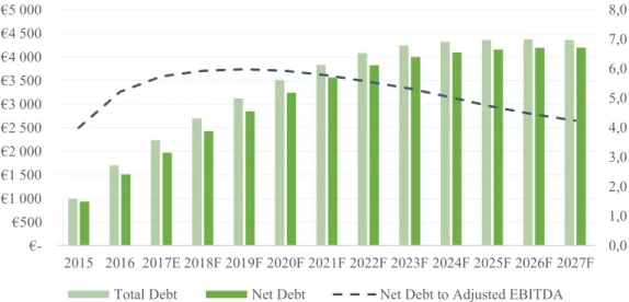
Debt is forecasted on a yearly basis regarding Cellnex’s financial position and a guideline for Net Debt to Adjusted EBITDA20. Net Debt to EBITDA is a common leverage ratio used to
analyze telecom related companies and it intends to show how many years it would take for the company to pay back its debt if net debt and EBITDA were held constant. Cellnex adjusts its EBITDA to the effects of Non-Recurring Items arising from M&A activity such as: Costs related to acquisitions; Tax associated with acquisitions; Lease Cancellation Costs; Prepaid expenses and Advances to Costumers.
To forecast debt through Net Debt to Adjusted EBITDA ratio, some assumptions also need to be made regarding cash holdings and adjustments to EBITDA. While the latter are estimated based on the Non-Recurrent Items value contribution per M&A PoP, the amount of cash the company holds in each period will be defined as a percentage of total operational costs – which, in 2016, represented, 44% of total operational costs. Even though this might seem excessive, when analyzing similar European companies we can see that they currently have cash holdings representing similar weights of their total operational costs21. Furthermore, in 2017’s half-year
results, Cellnex states that they have €567Mn in Cash (nearly 3x the cash position reported at year end 2016) and a total available liquidity of €1.6Bn (Cash + Credit Facilities). Hence, in the early years of our forecast we will assume a similar weight as its European Peers, which will experience a reduction as time goes by and business evolve.
20 Guideline of 6 to 6.5 (Max) for Net Debt to Adjusted EBITDA 21 See section Appendix 13 on Peers’ Cash Holdings
Figure 15 – Total debt and Net debt in €Millions and Net Debt to EBITDA ratio. Source: Own Calculations Interest expense is then calculated applying the before mentioned cost of debt to the total debt at the beginning of the year. In the table below are described both the interest amounts for each forecasted year and the corresponding Interest Tax Shields. The ITS Terminal Value was computed using the long-term growth rate of 1% and the cost of debt as discount rate following Myers (1970).
Table 6 – Interest Expense and Interest Tax Shields in €Millions. Source: Own Calculations
6.6 Bankruptcy Costs
Despite the benefits of increasing debt to capture Tax shields, high levels of debt might bring the company to a financial distress situation. If that happens, Cellnex will face some extra costs – bankruptcy costs - resulting not only from the need of contracting lawyers, consultants and other professionals to help overcome that situation (Direct costs) but also coming from the lack of confidence shareholders would have on the overall business (Indirect costs).
The methodology used to estimate Bankruptcy Costs consists in determining a Default Probability based on a Credit Default Swap and a Loss Given Default that expresses how much of the company’s value is lost in case it defaults. According to data available in Thomson Reuters terminal regarding Cellnex’s 5y CDS contract the Default Probability is 7.04% and the Loss Given Default is estimated to be 60% of company value.
0,0 1,0 2,0 3,0 4,0 5,0 6,0 7,0 8,0 €-€500 €1 000 €1 500 €2 000 €2 500 €3 000 €3 500 €4 000 €4 500 €5 000 2015 2016 2017E 2018F 2019F 2020F 2021F 2022F 2023F 2024F 2025F 2026F 2027F Total Debt Net Debt Net Debt to Adjusted EBITDA