Biogeochemical response of Tagus Estuary to climate change : a modelling study

(1)

Universidade de Aveiro 2015

Departamento de Física

Ana Rita Sá Longo

Biogeochemical response of Tagus Estuary to

climate change: a modelling study

Resposta biogeoquímica do Estuário do Tejo às

alterações climáticas

(2)

(3)

Universidade de Aveiro 2015

Departamento de Física

Ana Rita Sá Longo

Biogeochemical response of Tagus Estuary to

climate change: a modelling study

Resposta biogeoquímica do Estuário do Tejo às

alterações climáticas

Dissertação apresentada à Universidade de Aveiro para cumprimento dos requisitos necessários à obtenção do grau de Mestre em Ciências do Mar e das Zonas Costeiras, realizada sob a orientação científica do Prof. Doutor João Miguel Sequeira Silva Dias, Professor Auxiliar com Agregação do Departamento de Física da Universidade de Aveiro e co-orientação do Doutor Nuno Alexandre Firmino Vaz, estagiário de pós-doutoramento da Universidade de Aveiro.

Este trabalho foi desenvolvido no âmbito do projeto BioChangeR (PTDC/AAC-AMB/121191/2010).

(4)

(5)

o júri

Presidente _{Doutora Filomena Maria Cardoso Pedrosa Ferreira Martins}

Professora Associada do Departamento de Ambiente e Ordenamento da Universidade de Aveiro

Arguente _{Doutora Magda Catarina Ferreira de Sousa}

Estagiária de Pós-Doutoramento da Universidade de Aveiro

Orientador _{Doutor João Miguel Sequeira Silva Dias}

Professor Auxiliar com Agregação do Departamento de Física da Universidade de Aveiro

Co-Orientador _{Doutor Nuno Alexandre Firmino Vaz}

(6)

(7)

acknowledgements I could not have accomplished this MSc thesis without the friendship, help and advice of many people.

First, Prof. João Dias for being my supervisor, professor and friend since the beginning. My academic history would definitely have been a lot different. To Nuno Vaz, for all the help, the precious advice and suggestions and for introducing me to another one of my best friends during this thesis, MOHID.

Ana Picado, for pretty much everything, no words are good enough. To all the members of NMEC (Estuarine and Coastal Modelling Group) Magda, Leandro, Renato, João, Ana, Catarina and Carina for each day of advice, help and support.

To my friends since the beginning of my academic journey, especially, Américo e André.

To my parents, Domingos and Bela for all the love and support and for being the great sponsors of my academic path. To “Vó” Elisa and all the “Tias”. To Diana and Damião, in particular, for believing in me more than I usually do. Finally, to my “Migas” for keeping me sane and showing me that: “Pain is stepping on a nail (…) the rest is just being uncomfortable.

And you can sustain high levels of uncomfortable for a long time. (…) A big part of being successful is being uncomfortable”.

(8)

(9)

palavras-chave Clorofila-a; Estuário do Tejo; MOHID; modelo biogeoquímico; alterações climáticas.

resumo Os estuários são sistemas altamente dinâmicos que se encontram em risco devido a eventos relacionados com as alterações climáticas. Estas alterações podem ter impactos nos ciclos biogeoquímicos. Entre esses efeitos podem considerar-se o aumento de períodos de chuvas torrenciais e o aumento do nível médio do mar. Assim, o objetivo deste trabalho é o estudo do impacto destes eventos na dinâmica biogeoquímica do Estuário do Tejo, que se trata do maior sistema estuarino da Península Ibérica. Neste contexto, foi implementado, validado e explorado através de comparação com dados in-situ, um modelo biofísico 2D (MOHID). De forma a avaliar a resposta biogeoquímica do estuário a períodos de chuvas torrenciais, caracterizadas por variações abruptas nas descargas fluviais dos principais tributários, Tejo e Sorraia, foram considerados três cenários. O primeiro considerando um dia de descarga extrema para os rios Tejo e Sorraia. O segundo, considerando uma descarga extrema apenas para o Rio Tejo e por último, considerando uma descarga apenas para o Rio Sorraia. Relativamente ao aumento do nível médio do mar, foram estabelecidos dois cenários, o primeiro com o nível médio do mar atual e o segundo considerando um aumento de 0.42 m, conforme estimado em estudos anteriores. Os resultados para a simulação das chuvas torrenciais indicam que as modificações previstas para os padrões biogeoquímicos dependem essencialmente da descarga do Rio Tejo. Para o cenário de aumento do nível médio do mar os resultados sugerem uma diminuição da concentração de nutrientes e um aumento de clorofila em áreas específicas. Em ambos os cenários, o aumento de clorofila em determinadas zonas do estuário, sugerido pelos resultados, pode levar a eventos que promovam um crescimento anormal de fitoplâncton fazendo com que a qualidade da água diminua e colocando em risco todas as atividades que dependem no Estuário do Tejo.

(10)

(11)

keywords Chlorophyll-a; Tagus Estuary; MOHID;biogeochemical model; climate change.

abstract Estuaries are highly dynamic systems which may be modified in a climate change context. These changes can affect the biogeochemical cycles. Among the major impacts of climate change, the increasing rainfall events and sea level rise can be considered. This study aims to research the impact of those events in biogeochemical dynamics in the Tagus Estuary, which is the largest and most important estuary along the Portuguese coast. In this context a 2D biophysical model (MOHID) was implemented, validated and explored, through comparison with in-situ data. In order to study the impact of extreme rainfall events, which can be characterized by an high increase in freshwater inflow, three scenarios were set by changing the inputs from the main tributaries, Tagus and Sorraia Rivers. A realistic scenario considering one day of Tagus and Sorraia River extreme discharge, a scenario considering one day of single extreme discharge of the Tagus River and finally one considering the extreme runoff just from Sorraia River. For the mean sea level rise, two scenarios were also established. The first with the actual mean sea level value and the second considering an increase of 0.42 m. For the extreme rainfall events simulations, the results suggest that the biogeochemical characteristics of the Tagus Estuary are mainly influenced by Tagus River discharge. For sea level rise scenario, the results suggest a dilution in nutrient concentrations and an increase in Chl-a in specific areas.For both scenarios, the suggested increase in Chl-a concentration for specific estuarine areas, under the tested scenarios, can lead to events that promote an abnormal growth of phytoplankton (blooms) causing the water quality to drop and the estuary to face severe quality issues risking all the activities that depend on it.

(12)

(13)

xi| Contents

List of Figures

Figure 1: Tagus estuary 8

Figure 2: Monthly mean Tagus River discharge 10

Figure 3: Three nested domains used for the numerical simulations 16

Figure 4: Comparison of model results of ammonia, nitrate, oxygen and Chl-a with measurements 20

Figure 5: Discharges imposed on Tagus and Sorraia rivers 23

Figure 6: Mean time series of Chl-a concentration for the Scenarios #1, #2 and #3 24

Figure 7: Maxima Chl-a for Scenario #1 25

Figure 10: Sea surface elevation time series and instantaneous Chl-a, nitrate and phosphate

concentrations for the reference scenario in spring tide. 33

Figure 11: Instantaneous differences between reference and SLR scenarios for Chl-a, nitrate and

phosphate concentrations in spring tide. 34

Figure 12: Sea surface elevation time series and instantaneous Chl-a, nitrate and phosphate

concentrations along the entire estuary for the reference scenario in neap tide. 37 Figure 13: Instantaneous differences between reference and SLR scenarios for Chl-a, nitrate and

(16)

(17)

List of Tables |xv

List of Tables

Table 1: Values used as reference for the producers. 17

Table 2: Values used as reference for the consumers. 18

Table 3: Values used as reference for the decomposers. 18

Table 4: Scenarios description for torrential episodes. 22

(18)

(19)

Introduction|1

1. Introduction

1.1. Background and motivation

Estuaries are unique environments where the seawater meets freshwater, dictating the interactions between land and sea. Based on the Cameron and Pritchard (1963) classification an estuary is a “semi-enclosed coastal body which has a free connection with

the open sea and within which the sea water is measurably diluted with freshwater derived from land drainage”. Estuaries can be classified according to its topography, as coastal

plain estuaries (or drowned river valleys), bar-built estuaries, tectonic and glacier-carved. Coastal plain estuaries are the most common, formed by drowning of a former river valley either because of subsidence of the land or of a rise in sea level. The estuary studied in the present work, the Tagus estuary, is part of this group.

Estuarine dynamics and biogeochemistry are mainly driven by wind stress, wave regime, fluvial discharges, tide and nutrient inputs (Arndt et al., 2011). Major rivers are the main sediment contributors exporting a large amount of sediments into the sea and tide is responsible for exposing and/or submerging, for regular periods, some regions. These features interact and work on different time scales, but together they set constraints on biogeochemical function (Arndt et al., 2011).

Among the most important phenomenon that occurs in these systems are circulation and its impact in biogeochemical cycles and primary production. All the interactions and reactions in these systems can affect life in a large scale, which is more threatened over the years due to human and natural stress. Given the vast influence that biogeochemical cycles have on phytoplankton growth/decay and primary production, and on life in general, the study of the actual threats or those that these systems will face in the next years becomes a challenging matter of great interest. The main cause of the actual and future threats that coastal systems are facing is, among others, the climate change. According to the Intergovernmental Panel on Climate Change (IPCC), climate change is defined as “a

statistically significant variation in either the mean state of the climate or in its variability, persisting for an extended period (typically decades or longer). Climate change may be

(20)

2| Introduction

due to natural internal processes or external forcing, or to persistent anthropogenic changes in the composition of the atmosphere or in land use.”

The variations caused by climate change can be measured or predicted in terms of its effects on biogeochemistry, namely on nutrient cycles and phytoplankton growth, which are the major responsible for primary production in estuaries. In the surface, most of the primary producers are single cells or chains of simple cells. However, these organisms are responsible for more than 95% of the photosynthesis (Castro and Huber, 2007). The most important species in the net phytoplankton are diatoms and dinoflagellates. Diatoms commonly occur in nutrient-rich waters, near the coast or in open ocean. Dinoflagellates, are more abundant in warmer waters, and are able to grow better than diatoms under low-nutrient conditions. When low-nutrients are available, they can grow in large scale, resulting in blooms or even red tides (Castro and Huber, 2007), which can impact in estuarine and coastal systems, affecting the life cycle.

Primary production in marine environment is the result of the water masses movement coupled to nutrient and light availability. These elements can also limit production, either by absence or excess (Castro and Huber, 2007). These factors make the study and the attempt to predict these processes highly relevant to become aware of the threats faced by estuaries.

Regarding light, it is known that the primary production can be light limited and depends on the intensity of light that arrives to the first layers and how far the light can penetrate in the water column, i.e. photic zone, which varies with the year season and local weather conditions.

As previously referred, nutrient availability has also a major role on primary production. In their absence, even if there is a large amount of light available, photosynthesis can be limited or even does not occur and the production becomes nutrient limited.

Estuaries with a relative shallow depth that receives freshwater input from the rivers are usually highly productive areas because of the balance between the depth of the photic zone and the nutrient availability (Castro and Huber, 2007).

The morphology of the Portuguese coast is characterized by several estuarine systems that throughout the centuries, and mostly between 1415 and 1543 during the “Era dos

(21)

Introduction|3

in the country (namely Lisbon). Among the largest estuarine systems along the Portuguese coast, the Tagus Estuary is located near Lisbon, the capital city, being located in the geographical area with the highest population density in Portugal (38° 44’ N, 9°08’ W). The Tagus estuary is considered a mesotidal system with semi-diurnal tides, a surface area of 320 km2 and a mean volume of 1900×106 m3. The inflow of saline water from the Atlantic Ocean along with the riverine input of freshwater, determines the hydrographic conditions of the estuary.

The particular conditions of Tagus estuary make it a relevant study case. It is one of the largest estuarine systems in Europe, the largest in Portugal and it involves 18 municipalities in the metropolitan area of Lisbon. It has around one million inhabitants that depend on it either on a direct or indirect way (Guerreiro et al., 2015). In addition, it harbors a major port and a shipping terminal with about 3000 large vessels entering the harbor annually, named “Porto de Lisboa”. The estuary has an important economic relevance in areas as trade, maritime traffic, dredging, industry and fisheries (Guerreiro et

al., 2015). All these estuarine uses may provoque a high human stress, turning the study of

the Tagus dynamics an important and actual issue.

In order to study the threats that the Tagus estuary might face, because of climate change, numerical modeling results can give a valuable support to major decisions, such as the design of ports, sewage systems and ecological reserves (Neves, 2007). In order to qualify as a Decision Support Tool, a model must have a good performance in producing results that describe a reference situation and hypothetical scenarios (Neves, 2007).

1.2. Aims

The main aim of this work is to study the climate change impact in the biogeochemical response of the Tagus estuary in terms of chlorophyll-a (Chl-a) and nutrients (nitrate and phosphate). In order to achieve it, some specific objectives were established:

 To characterize the hydrography and dynamics of the Tagus estuary under different forcing conditions;

 To use a biogeochemical module coupled to a hydrodynamic model MOHID to evaluate biogeochemical features;

(22)

4| Introduction

 To study the influence of climate change, by studying the response of the estuary to torrential episodes and sea level rise, on Chl-a and nutrients inside the estuary;

 To determine the time response and the relaxation period of the estuary to torrential episodes characterized by extreme fluvial discharge events;

1.3 State of the Art

In this section a literature survey on biogeochemical modelling studies, and on Tagus Estuary modelling and biogeochemistry along with the characteristics of study area is presented.

1.3.1 Tagus Estuary

In the last years, Tagus estuary particular conditions and increasing economic and social relevance made it a relevant case study.

Considering the last years, the tidal currents on the mouth of Tagus Estuary using a three-dimensional nested model and performing a comparison with field data were investigated by Fortunato et al., (1997). From this application, new insights into barotropic circulation were obtained at the mouth of the estuary.

Vaz et al., (2009) researched the Tagus estuarine plume using three-dimensional nested models. The results suggest that estuarine waters form a plume influenced by the morphology of the coastline.

In order to study the dynamics and hydrology of the Tagus estuary to increase the understanding of the tidal propagation inside the estuary, the thermohaline and circulation patterns and the role of the principal forcing mechanisms of the estuarine dynamics, Neves, (2010) carried out a study. This study was based on an analysis of an observational data set and this study promoted the clarification of the link between the thermohaline and circulation patterns and the corresponding forcing mechanisms, and contributed to clarify aspects about the tidal asymmetry.

Dias and Valentim, (2011) studied the Tagus estuary tidal dynamics by performing an analysis of the amplitude, phase and tidal ellipses of the main semi-diurnal and diurnal tidal constituents. The study was carried out using a 2D vertically integrated model. Then,

(23)

Introduction|5

a harmonic analysis of the model results was performed. Results suggest that the most important diurnal and semi-diurnal constituents are M2 and K1, respectively, and it was

observed that the variations in amplitude occur where changes in morphology and depth are more significant. The ellipses orientation reveal the importance of the bottom topography and bay geometry, on the tidal fluxes. Model shows that the tidal dynamics of the system is extremely dependent on estuarine topography and coastline features, resulting essentially from a balance between convergence/divergence and friction effects, and from an estuarine resonance mode with a period close to twelve hours.

Regarding the residual currents and transport pathways in the Tagus estuary, Vaz and Dias, (2014) aimed to investigate the residual flows considering the major forcing factors (tide, river discharge and wind stress). The study was carried out using an high resolution estuarine model set in a 2D way, to simulate the tidal dynamics of the estuary. The tidal flows were calculated by tidally averaging the flow currents along the whole estuary. The complex bathymetry, tides, river discharge and wind stress modulate the residual flow. The effect of the tide combined with river discharges sets preferential corridor flows in the deeper areas. For the shallow areas, near the south shore of the estuary is the wind intensity and direction that dictates the changes in the residual currents. River runoff changes the residual current intensity. The wind direction also induces changes in the residual flow patterns, inducing a rotation of the residual flow according to the wind direction.

Then, the evolution of hydrodynamics in the Tagus estuary in the 21st century by analyzing the effects of sea level on tidal propagation and circulations and its consequence on sediment dynamics, water quality and extreme water levels was studied by Guerreiro et

al., (2015). The study was carried out with a shallow water model and the results show that

sea level rise will significantly affect tidal asymmetry, in particular because the intertidal area can decrease by 40 % by the end of the 21st century. As consequence, the ebb-dominance can be reduced. Moreover, the resonance in Tagus can be enhanced causing extreme water levels to be higher than in the present.

1.3.2 Biogeochemical modelling

Model results give valuable information that could support decisions, provide forecast of estuarine dynamics and biogeochemistry and allow the comprehension of different processes that occur in estuaries.

(24)

6| Introduction

Biogeochemical models were largely developed benefiting from the scientific and technological progress and have been coupled to physical (hydrodynamic) models thus generating the present integrated tools (Neves, 2007).

Regarding the modelling of biogeochemical processes, there is a study by Xu et al., (2006) that describes the development and validation of a simple biogeochemical model for the Chesapeake Bay in order to evaluate the model performance in representing dissolved inorganic nitrogen, phytoplankton, dissolved oxygen, total suspended solids and light attenuation coefficient. A dry and a wet year were chosen and the results were compared with observations. They found that the model was robust enough to generate reasonable results under both dry and wet conditions despite some observed discrepancies, such as an overestimation of phytoplankton in shoal areas and some overestimation of oxygen in deeper channels.

In order to study the phytoplankton and nutrient dynamics in Tagus Estuary, Mateus et

al., (2008) showed the importance of light on primary production, using a process-oriented

ecological model for the water column, coupled with a 2D hydrodynamic model. The results suggest that in an estuary like Tagus, the main limiting factor is not nutrient concentration but light availability. Thus, nutrient limitation is only confined to some areas on the lower estuary and in summer.

The study by Arndt et al., (2011), presents an attempt to quantify biogeochemical parameters along the entire Scheldt estuary in the Netherlands, using a 2D, nested-grid hydrodynamic model coupled to MIRO model for the coastal zone and CONTRASTE model for the estuary. The results show that there is a balance between the estuary and the coastal zone in terms of estuarine nutrient inputs. Moreover, it shows that the coastal diatoms intrude upstream into the saline estuary. This intrusion tends to reduce nutrient concentrations in the estuary, reinforcing nutrient limitation on the coastal zone.

Mateus (2012) study, aims to formulate a set of equations describing pelagic biogeochemical processes disregarding physical processes (which are already set on the numerical model used and described on the companion paper. According to this study, ecological models have been constructed in the last few decades, with different levels of detail. This model differs from others because instead of modelling distinct types of organisms for each Living Functional Group, a Generic Type Model is chosen which allows the user to define the number of types in each Living Functional Group. There is

(25)

Introduction|7

also an option to account for silica dynamics and mixotrophy (using photosynthesis and heterotrophy combined) on producers. This model was developed as a component of MOHID Water Modelling System (MWMS) and it is sufficiently generic to be applied to different marine ecosystems. The study applies the previous model coupled to MWMS in the Tagus Estuary and analyses its performance in studying physical, chemical and environmental parameters on the biogeochemistry of Tagus Estuary. In addition, it tries to accomplish two major objectives: develop and implement a coupled system capable of reproducing biological and physical characteristics and create a coastal management tool based on the integration of model and in-situ data. The results suggest that the model has a good performance capturing the complexity of the estuary and the ecological patterns. Then in a companion study, Mateus et al.(2012) used an integrated ecosystem model to study the role of physical, chemical and environmental parameters on the biogeochemistry of Tagus estuary. The results suggest that the model used captures the complexity of Tagus estuary and provides reasonable estimates of the biomass trends of a highly dynamic and interactive community.

In order to study the influence of Tagus estuary on the near coastal system, Vaz et

al., (2015) used a model application, which allows the description of the main physical and

biogeochemical processes in the region of freshwater influence. This work was carried out using a nested modelling approach. The results suggest an adequate reproduction of the vertical thermal structure and chlorophyll concentrations and a reasonable agreement for water temperature. Chlorophyll vertical profiles show some differences between the model results and bibliography.

Also, Lopes et al., (2015) aimed to assess the state of the trophic web of a temperate lagoon in Portugal in situations of nutrients limitation that can occur during extreme weather events. These authors used an ecological/eutrophication model integrating nutrient cycling and main phytoplankton processes. Results suggest that changes in light or nutrient availability can seriously modify the lower level state of the lagoon trophic level dynamics.

(26)

8| Study area: characterization of the Tagus estuary

2. Study area: characterization of the Tagus estuary

2.1. Tagus estuary

The Tagus estuary (Figure 1) has a total surface area of 320 km2 and a mean volume of 1900 × 106 m3 and is a relatively shallow mesotidal estuary with semi-diurnal tidal regime in which the circulation is mainly tidal driven (Vaz et al., 2011). The mean tidal amplitude is 2.2 m, ranging from 1 m (neap tide) to 4 m (spring tide) and it increases throughout the estuary (Mateus and Neves, 2008). M2 is the dominant tidal constituent with amplitudes of

1 m and the surface velocities are approximately 1 m s-1.About 20 to 40% of the estuarine area is characterized as intertidal areas, composed mainly by tidal flats that are known to have an important role in the estuary hydrodynamics features by modifying the tidal wave and on biogeochemical features by promoting primary production (Fortunato et al., 1999). The estuary is also characterized by the existence of sand beaches, both in inlet channel and in the inner bay (Freire and Andrade 2008). It is a well-mixed estuary due to the interactions between strong tidal currents and high input of river water. Stratification happens rarely, only in specific situations such as neap tides or after heavy rainfall (http://www.maretec.mohid.com/portugueseestuaries/tagus/Tagus.htm).

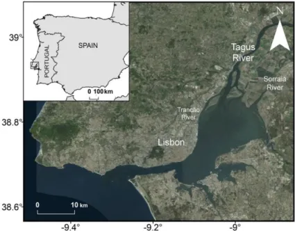
Figure 1: Tagus estuary with the location of the main city (Lisbon) and the main rivers (Tagus, Sorraia and Trancão).

(27)

Study area: characterization of the Tagus estuary|9

The seasonal variability of the river discharge has influence on the residence time of the estuary, which was found to be between 6 and 65 days for a river discharge between 100 m3s-1 and 2200 m3s-1, and 23 days for a river discharge of 350 m3s-1 (Neves, 2010a).

The hydrodynamic conditions are determined by the balance between the inflow of saline water from the Atlantic Ocean and the riverine discharges from the three contributors, Sorraia, Trancão and Tagus Rivers (Figure 1), being the Sorraia and Tagus Rivers the main tributaries and the last the most significant in terms of riverine flow and urban, industrial and agricultural effluent discharges.

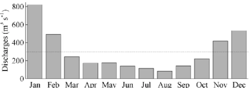
Tagus River is the most important source of freshwater into the estuary. It is located in the middle of the Iberian Peninsula and it runs in a northeast-west direction for 1038 km. The monthly mean Tagus River discharges for the years between 1990 and 2000 are displayed on Figure 2, considering data from Sistema Nacional de Informação de Recursos Hídricos (SNIRH) (http://www.snirh.pt). Generally, discharges show a typical pattern, with high values during winter and low values during summer. Tagus River presents an average discharge of 300 m3 s-1 with variations from summer to winter, being the minimum value of 82 m3 s-1 in August and the maximum value of 820 m3 s-1 in January for the period 1990-2000. According to Neves (2010) variations can range from 30 m3 s-1 for a dry summer, to 2000 m3 s-1 for a wet winter. However, extreme values of about 15000 m3s-1 for instantaneous maximum flows were found (Vaz et al., 2009).

The Sorraia River has an area of 7556 km2, and is considered the largest basin inside the Tagus River basin. The River forms in Couço, because of the confluence of the rivers Sor and Raia and it flows in a west direction towards the Tagus estuary. It has a total length of 155 km and a mean flow of approximately 39.5 m3 s-1, which represents less than 15% of the Tagus river discharge. Sorraia drains a plane known by having an intense agricultural activity (http://www.maretec.mohid.com/portugueseestuaries).

Trancão basin is located at the northern limits of Lisbon, covering an area of 300 km2 and constituting an important tributary to Tagus Estuary (Carreira et al., 1999). It has a flow of about 5 m3s-1 . Although it is a small basin, it is densely urbanized. The region has been modified by industrial, domestic and agricultural discharges in the 70s, however the water from Trancão is an important source for irrigation purposes (Carreira et al., 1999). It has a small natural flow when compared with the other tributaries, Tagus and Sorraia.

(28)

10| Study area: characterization of the Tagus estuary

Figure 2: Monthly mean Tagus River discharge (m3s-1) from 1990 to 2000. The dashed line represents the average.

The limiting nutrients are known to be nitrogen and silica and those are never depleted inside the estuary (Mateus and Neves, 2008). Nutrient limitation is only significant in lower estuarine areas and mostly during summer. Light is believed to be the main factor controlling the primary production on Tagus Estuary, given that the carbon to nutrient ratios only drop below the Redfield ratio, on rare occasions (Mateus and Neves, 2008).

(29)

Numerical model MOHID|11

3. Numerical model MOHID

The present study was performed using MOHID (www.mohid.com), a numerical model developed by MARETEC (Marine and Environmental Technology Center – Instituto Superior Técnico).

MOHID is characterized as a three-dimensional baroclinic finite volume model, designed for coastal and estuarine shallow water application (Leitão et al. 2005; Vaz et al., 2005; Vaz, 2007). The model solves the three-dimensional incompressible primitive equations and assumes the hydrostatic equilibrium as well as Boussinesq and Reynolds approximations (Valentim et al., 2013). Along the Portuguese coast, MOHID has been applied to different environments, from coastal lagoons like Ria de Aveiro (Vaz et al., 2005; Vaz et al., 2007) to estuaries like Sado (Martins et al., 2001) and Tagus and Tagus plume (Vaz et al. , 2009; Vaz et al., 2011) and it as shown a good performance simulating its intricate features (Vaz, 2007). In order to perform the simulations required for this study and given the intense vertical mixing, a validated MOHID 2-D depth integrated model for the Tagus Estuary was used.

Mohid Life is a multi-parameter biogeochemical model based on ERSEM that is used coupled to MOHID and simulates nutrients, primary producers, secondary producers and decomposers. The model is a twelve-component pelagic biogeochemical model which comprises, producers, consumers, decomposers, organic matter (particulate, dissolved labile and semi-labile), nutrients (nitrate, ammonium, phosphate, silicate acid), biogenic silica and oxygen. Trophic interactions are expressed in terms of material flow of basic elements (like carbon and nutrients). Producers, consumers and decomposers are considered as Living Functional Groups (LFG). These are composed by an assemblage of organisms with different roles in the biogeochemical processes (Mateus, 2012).

(30)

12| Numerical model MOHID

3.1. Governing equations

3.1.1. Circulation model

MOHID solves the three dimensional incompressible primitive equations, considering the hydrostatic equilibrium and Boussinesq and Reynolds approximations. The momentum and mass balance equations are given by:

(1) (2)

In these equations, is the velocity vector in the horizontal Cartesian directions (i = 1,2), is the velocity vector component in the three Cartesian directions (j = 1-3), is the atmospheric pressure, is the turbulent viscosity. represents the specific mass and the specific mass anomaly. is the reference specific mass, is the free surface level, is the specific mass on the free surface, g is the acceleration of gravity, t the time, the Earth’s rotation velocity and the alternate tensor.

The free surface equation is obtained integrating equation (2) along the water column, being h the depth.

(3)

A more detailed description of the governing equations for MOHID can be found in Santos, (1995); Leitão, (2003) and Vaz, (2007).

3.1.2. Biogeochemical model

Models working with marine physical and biological interactions have to consider both the physical processes (transport, light and temperature) and the biochemical, because the concentration of the variables is function of both. Transport processes conserve the total quantity of transported variables, while biological and chemical processes are non-conservative (one variable is converted into another). The model complies with the mass

(31)

conservation principle and so, while state variables are not conserved, carbon, nitrogen, phosphorus and silica are. The evolution over time of each variable is described by equation 4:

– phy – bio (4)

In equation 4, C is a given concentration of a state variable as a continuous function of space and time and a generalized flux of the property. This flux is composed by a physical ( phy) and a biogeochemical component ( bio). The first term of the equation 4

represents the alterations to the property concentration caused by physical processes such as vertical and horizontal advection and diffusion effects. The second term represents the changes in the property controlled by biological and geochemical processes.

The water motion dynamics is ruled by the equations of fluid dynamics, linking the transport processes with biogeochemical components. The transport of any given property is given by the advection-diffusion (Equation 5):

– – – (5)

In this equation, Ux,y,z represents the water velocity in a three-dimensional referential,

and Dx,y,z the turbulent diffusion coefficients in each direction. Physical processes are

resolved by the hydrodynamic module in MOHID. Finally, F(C,t) addresses the loss/gain term of the property calculated by the biogeochemical model. The available light energy at the surface I0 (W m

-2

) or incident short wave radiance can be calculated for a given geographic location or a set of measurements can be used to force the model instead. The specific amount of solar radiation available for a control volume is calculated by the model by estimating the absorption of light in the water column above and within the control volume itself. This is obtained knowing the total absorption coefficient and the water column height. The incident radiation is considered when the control volume is at the surface. It is assumed that the light gradient follows Lambert-Beer law (Equation 6):

(32)

(6)

The net extinction coefficient for the photosynthetic active radiation (PAR) in Equation 7 is the sum of each individual contribution of water molecules, chlorophyll, DOMc (labile plus semi-labile) and POMc absorption, each with the respective extinction

factor ɛ* :

(7)

If more than one type of producers is defined, the total chlorophyll a is used, calculated as , where i is a phytoplankton type, the chlorophyll content of that type and n the total number of types.

The canonical equation which describes the net growth of a stadar organism is given by:

(8)

In this expression, Xc represents the carbon biomass of the standard organism which

depends on the specific uptake (up), specific total respiration rate (rsp), specific mortality (mrt), specific total excretion rate (exc), and on the grazing rate. Xc are the producers’ (Pc),

consumers’ (Zc) or decomposers’ (Bc) biomass. Uptake and predation processes are defined

as a linear function response to substrate or prey density and a simple encounter mechanism is used to govern prey consumption kinetics. Mortality rate is density independent. Standard organism biomass is carbon-based and defined by the element content (C, N, P, Si and Chl-a) (Mateus, 2012).

3.2. Model Implementation

In order to perform the necessary simulations for this study, the model was implemented using a downscaling methodology, with nested domains, previously used and explained by Leitão et al., (2005) and Vaz et al.,(2011).

(33)

The model uses three levels of nested grids with different resolutions (Figure 3). The first domain (D1) is a 2D barotropic tidal driven model forced by the FES2004 global solution, which covers up most of the Atlantic Coast (from 33 to 50ºN and 0 to 13ºW) and has a horizontal resolution of ~6 km. The time step used was 180 s. The second domain (D2) comprises a region from 8º30’ to 10º30’W and 36 to 40ºN, with a horizontal resolution of ~1.6 km and a time step of 60 s. Finally, the third domain (D3) includes the whole Tagus estuary area (from 38º30’ to 39ºN and 8º42’W to 9º30’W) and is directly coupled to D2 at the open boundary. It has a numerical grid with 335×212 cells with a horizontal resolution of 200 m. The time step was set to 15 s and the horizontal viscosity to 5 m2 s-1. D3 is forced by the tide from D2. Both D2 and D3 are two-dimensional models.

(34)

Figure 3: Three nested domains used for the numerical simulations, with bathymetry in meters. Location of the calibration stations (S1, S2, S3 and S4) and location of the local station of time series

analysis (white triangles).

Atmospheric forcing consisting in wind direction and intensity, radiation, air temperature, relative humidity and precipitation data was imposed with an hourly temporal resolution. These data were obtained at a nearby meteorological station: Estação Meteorológica da Guia (http://www.mohid.com/tejo-op/).

The Tagus River discharges were provided by Sistema Nacional de Informação de Recursos Hídricos (SNIRH, www.snirh.pt). Due to the lack of data for Sorraia and Trancão rivers, climatological values were imposed .

In order to simulate the biogeochemical features of Tagus estuary, the module Life was coupled to the hydrodynamic model. The biogeochemical model was only considered in D3 domain, following the procedure developed by Vaz et al., (2011) and Mateus (2012).

The ecological model iterates every 3600 s and homogeneous initial conditions for the ecological model properties were derived from National Oceanographic Data Center (NODC) climatological data. Therefore, a one-year run was performed to ensure that the results were independent from the initial conditions. The riverine inputs for biogeochemical variables (including nutrients, biological constituents and dissolved matter) were calculated from SNIRH data sets.

The model was built around the Generic Type Model (GTM) concept, which is a strategy that allows the definition of the number of types inside each LFG, instead of using a fixed trophic structure. For each LFG this arrangement allows the modelling of n types or species different nutrient dependencies, trophic relations mixotrophic behavior, rate values, etc., while sharing the same set of equations. Each type is specified by a set of parameter values, trophic relations and processes (Mateus, 2012). For this simulation, two types of producers were considered. These producers are diatoms and autotrophic flagellates, which are able to perform photosynthesis. The consumers are microzooplankton, which have a predatory action on the producers. This division in two groups of producers was based on nutrient and trophic relations. Parameter values for each GTM are listed in Tables 1 to 3 and are based on Mateus et al., 2012.

(35)

Numerical model MOHID|17 Table 1: Values used as reference for the producers.

Producers (Diatoms and autotrophic flagellates)

Parameter Value Units

Redfield N:C ratio 0.176078 mg N (mg C)-1 Minimum N:C ratio 0.088038 mg N (mg C)-1 Maximum N:C ratio _0.35215536 _{mg N (mg C)}-1 Redfield P:C ratio 0.024342 mg P (mg C)-1 Minimum P:C ratio _0.01217121 _{mg P (mg C)}-1 Maximum P:C ratio 0.04868484 mg P (mg C)-1

Standard Si:C ratio _0.8427 _{mg Si (mg C)}-1

Chla specific initial slope of the

photosynthesis-light curve 0.002 mg C m

2_{(mg Chla W d)}-1

Maximum Chl:N ratio 0.214 mg Chla (mg N)-1

Q10 value 2.0 -

Maximum assimilation rate _1.2;1.7 _d-1

Exudation under nutrient stress 0.05;0.2 -

Basal respiration rate 0.15;0.1 d-1

Respired fraction of production 0.1;0.25 -

Minimum lysis rate 0.05 d-1

Nutrient stress sedimentation rate _5.0;0 _{m d}-1

Minimum sedimentation rate ₀ _{m d}-1

Nutrient stress threshold 0.70;0.75 -

Maximum rate of storage filling 1 -

Affinity for NO3 2.5×10-6 (mg C)-1 l-1 d-1

Affinity for NH4 2.5×10-6 (mg C)-1 l-1 d-1

Affinity for PO4 2.5×10

-6

(mg C)-1 l-1 d-1

Release rate of exces silicate 1 d-1

Silicate uptake Michaelis constant 0.0084 mg Si l-1

DOM fraction diverted to semi-labile

(36)

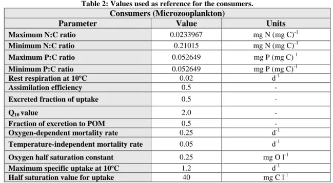
Table 2: Values used as reference for the consumers. Consumers (Microzooplankton)

Maximum N:C ratio 0.0233967 mg N (mg C)-1 Minimum N:C ratio 0.21015 mg N (mg C)-1 Maximum P:C ratio 0.052649 mg P (mg C)-1 Minimum P:C ratio 0.052649 mg P (mg C)-1 Rest respiration at 10ºC 0.02 d-1 Assimilation efficiency 0.5 -

Excreted fraction of uptake 0.5 -

Q10 value 2.0 -

Fraction of excretion to POM 0.5 -

Oxygen-dependent mortality rate 0.25 d-1

Temperature-independent mortality rate 0.05 d-1

Oxygen half saturation constant 0.25 mg O l-1

Maximum specific uptake at 10ºC 1.2 d-1

Half saturation value for uptake 40 mg C l-1

Table 3: Values used as reference for the decomposers. Decomposers

Maximum N:C ratio 0.2762 mg N (mg C)-1

Minimum N:C ratio 0.2333 mg N (mg C)-1

Maximum P:C ratio 0.0516 mg P (mg C)-1

Minimum P:C ratio 0.0339 mg P (mg C)-1

Rest respiration at 10ºC 0.01 d-1

Maximum specific uptake at 10ºC 6.0 d-1

Half saturation constant for DOM uptake 0.001 mg C l-1

Assimilation efficiency 0.3 -

Assimilation efficiency at low oxygen 0.2 -

Q10 value 2.95 -

Fraction of mortality products to POM 0.4 -

Fraction of DOM to semi-labile pool 0.2 -

Density-dependent mortality rate 0.5 d-1

Density independente mortality rate 0.05 d-1

Mortality density dependent reference

concentration 0.05 mg C l

-1

Oxygen half saturation constant 0.01 mg O l-1

Oxygen concentration below which ass = assef low 1.6 mg O l-1 Affinity for NO3 2.5×10 -6 _{(mg C)}-1_l-1_d-1 Affinity for NH4 2.5×10 -6 (mg C)-1 l-1 d-1 Affinity for PO4 2.5×10 -6 _{(mg C)}-1_l-1_d-1

Maximum rate for POM hydrolysis 1 d-1

Maximum rate for DOMsl hydrolysis 1 d-1

POM hydrolysis half saturation constant 0.032 mg C l-1

DOMsl hydrolysis half saturation

constant 0.2 mg C l

(37)

Numerical model MOHID|19 3.3. Validation

The hydrodynamic model of the present implementation was already validated in Vaz

et al. (2011), which obtained differences less than 5% for the semi-diurnal M2 and diurnal

O1 constituents and 5º for the phase. Therefore, it was assumed that the physical

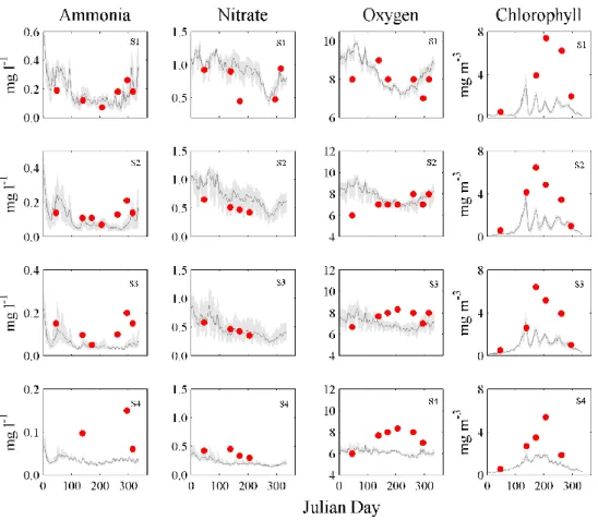
parameters were correctly simulated. Thus, only the biogeochemical parameters are qualitatively compared with available measurements of nutrients, oxygen and chlorophyll. Initially, a simulation covering the period from April 2003 to December 2004 was performed and the biogeochemical properties, including nutrients, Chl-a and oxygen concentrations, were qualitatively compared with measured data at stations S1, S2, S3 and S4 (Figure 2 - D3). The data used for the comparison are described in Mateus et al. (2012) and Mateus and Neves (2008).

Results are presented in Figure 4, where the grey area represents the area comprised between the daily maximum and minimum model predictions of each variable and the dark grey line represents the daily mean of those variables. Measured data are represented by the dots.

The model results reveal a strong seasonality in ammonia concentrations, especially for stations S1 and S2, with higher values in winter and lower in spring and summer (see Figure 4), showing good general agreement with observations. Indeed, despite some differences on ammonia at station S4, the model correctly reproduces the simulated trends. However, predictions are slightly lower than the observations.

Model nitrate concentrations also show a marked seasonality, on stations S1 to S3, with higher values in winter (>1 mg m-3) than in summer (0.5 mg m-3).

According to Figure 4, it can be concluded that the model represents well the nitrate dynamics, however, overestimating observations. In general, predicted oxygen trends reproduces well the data on S1 and S2, with mean values between 8 and 10 mg l-1. For stations S3 and S4, the model underestimates oxygen during summer months with a mean value around 7.5 mg l-1, when the measured data suggest a peak of around 9.5 mg l-1 in oxygen concentration. However, the model is still able to capture and reproduce a slight increase of the oxygen concentration, around the same time that the measure data values start to increase.

(38)

Figure 4: Comparison of model results (grey shadowed area and grey line) of ammonia, nitrate, oxygen (mg l-1) and Chl-a (mg m-3) with measurements for all the calibration stations (S1, S2, S3, S4).

Finally, the predicted Chl-a concentration also show high seasonality, with high values occurring in late spring/early summer, with maxima values of 4 mg m-3. In this case, model results are, in general, lower than observations.

The differences observed between the model and the measured values, are probably because the biogeochemical variables depend on one another, so if the model underestimates one variable, the other variables will also present different values. Furthermore, the differences on S4 can be explained by the fact that this station is located on the estuary mouth channel, the closest to the coastal zone (Figure 3) and thus, in the most dynamic zone of the estuary.

In order to validate a different implementation of MOHID in the study area, Mateus and Neves (2008) used the same data set and similar results were achieved.

(39)

(40)

22| Biological response of Tagus Estuary to climate change

4. Biological response of Tagus Estuary to climate change

In this chapter, the biological response of the Tagus estuary to climate change, considering the effects of torrential episodes and sea level rise, through numerical modelling is evaluated.

4.1. Impact of torrential episodes

As the main goal of this section consisted in investigate the biological response of Tagus estuary to extreme freshwater discharge induced by torrential episodes, three scenarios were set defining extreme values of the main tributaries: Tagus and Sorraia. Trancão river was not included in these scenarios considering that its flow is negligible and consequently without impact in the general biogeochemical patterns of the estuary.

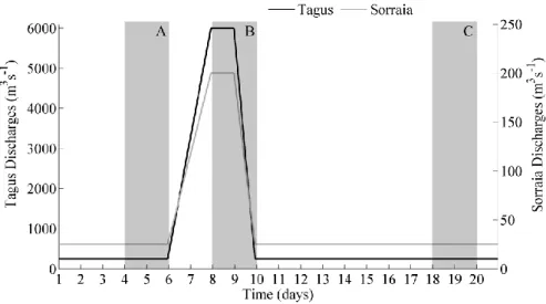
Primarily, a scenario considering one day of extreme discharge for the Tagus (6000 m3s-1) and Sorraia (200 m3s-1) rivers was considered (Scenario #1). Next, in order to assess the impact on the estuarine biogeochemistry of the freshwater discharge from each river separately, two more scenarios were defined: Scenario #2, considering only high discharge from Tagus and Scenario #3, considering only high discharge from Sorraia River, as it is summarized in Table 4. The simulations were conducted for March of 2004.

The freshwater discharges considered in this study are depicted in Figure 5. They were set based on: between days 6 and 8, discharges from both rivers linearly increase from a base flow (250 m3s-1 for Tagus and 25 m3s-1 for Sorraia), to a peak value (6000 m3s-1 for Tagus and 200 m3s-1 for Sorraia).

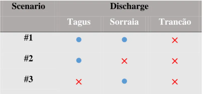
Table 4: Scenarios description for torrential episodes (the blue dots represent the discharges considered and the red crosses represent the discharges neglected, for each scenario).

Scenario Discharge

Tagus Sorraia Trancão

#1

●

● _×

#2

● _×

_×

(41)

Biological response of Tagus Estuary to climate change|23

Figure 5: Discharges imposed on Tagus and Sorraia rivers (m3s-1). A, B and C represent the periods for which the results are evaluated.

Then, they remain constant during a day (from day 8 to 9), and then decrease, during one day, to the base flow again. The mean and maxima values used to impose the discharges, were determined based on 24 years time series (1990-2014). This pattern was defined to assess the estuarine response to torrential episodes and evaluate its behaviour under the relaxation period.

All simulations were performed for 20 days, to evaluate Chl-a and nutrients concentration distribution and temporal evolution as well as the relaxation period to extreme discharges.

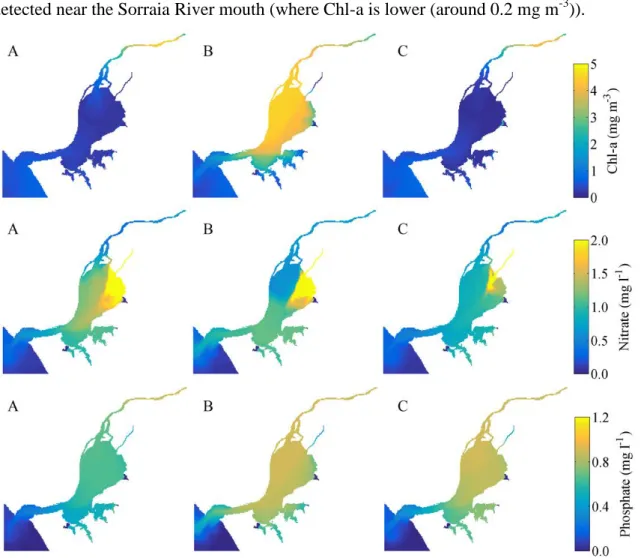
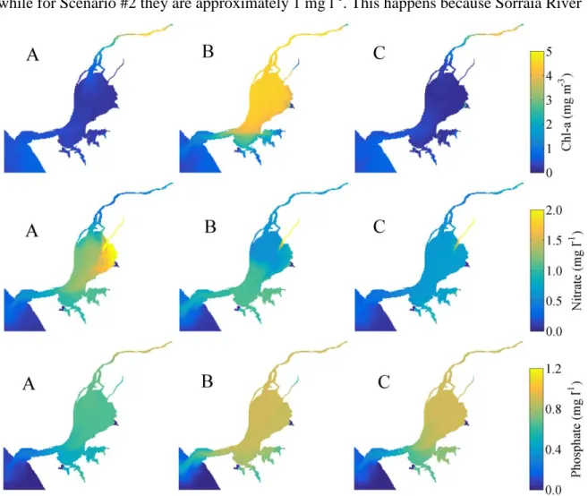
From numerical predictions, Chl-a and nutrients (nitrate and phosphate) maxima concentrations were computed for each cell of the estuarine numerical grid for three different periods: before the peak flow (A), in the peak flow (B) and after the peak (C). The results are primarily analyzed in terms of Chl-a time series, since this variable is assumed to be a natural bio-indicator, considering its complex and rapid response to changes in environmental conditions such as nutrient and/or light availability (Livingston, 2001).

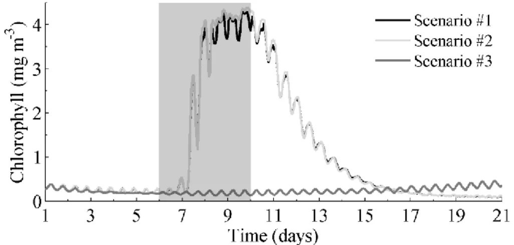
Figure 6 depicts the mean Chl-a concentration time series at six stations located in the central area of the estuary (triangles in Figure 3), in order to understand the general Chl-a trend. Chl-a concentration follows the same trend as the imposed discharges for Scenarios #1 and #2. However, a time delay between Chl-a and the extreme discharge close to one

(42)

day was found (discharges increase from day 6 and Chl-a from day 7 – Figure 6). Two days after the imposed discharge, Chl-a levels remain high, oscillating around 4 mg m-3

Figure 6: Mean time series of Chl-a concentration for the Scenarios #1, #2 and #3 (mg m-3). The shaded area represents the period of extreme discharges.

during approximately 3 days, then it decreases to the base value, with concentrations lower than 0.5 mg m-3 after seven days. It is noteworthy that the mean values of Chl-a concentration after the relaxation period are slightly lower than the ones observed before the imposed extreme discharges. For Scenario #3, when an extreme discharge is imposed only in Sorraia River, the pattern is completely different: Chl-a concentration slightly increase from day 7 to the end of simulation.

From the analysis of the time series, and the extreme discharge period it seems obvious that the discharge has a great influence on the Chl-a behavior in the estuary. The time response of Chl-a to the extreme discharge is of about one day and the relaxation period starts approximately one day after the torrential episode cessation and ends five days later.

Based on these results, Chl-a and nutrients (nitrate and phosphate) maxima were calculated and their values assessed for the three scenarios and for three periods, one before the high discharge (A), other during the peak (B) and a third period after the relaxation period (C).

For Scenario #1, before the extreme discharge (period A) low maxima Chl-a concentrations were found in the whole estuary (Figure 7 – upper panel A), with values ranging from 0.2 mg m-3 on the middle estuary to 1.0 mg m-3 on the upper estuary (right next to the Tagus River mouth) and on the estuary mouth. As the Chl-a concentration is low, nutrients (nitrate and phosphate) are expected to present high values. Indeed, high

(43)

nitrate concentrations are found in the whole estuary, with the highest values (2.0 mg l-1) detected near the Sorraia River mouth (where Chl-a is lower (around 0.2 mg m-3)).

Figure 7: Maxima Chl-a (top panel), nitrate (middle panel) and phosphate (bottom panel) concentrations for periods A, B and C (Figure 4) and for Scenario #1.

Phosphate concentrations are relatively uniform along the estuary, with mean values about 0.8 mg l-1. These results are in accordance with those obtained by Mateus et al. (2012), who found relatively low concentrations during winter in the estuary (ranging from 0.8 to 1.0 mg l-1, except on the Sorraia River mouth where the values reach 1.5 mg l-1 for nitrate and ranging from 0.4 to 0.8 mg l-1 for phosphate), and concluded that the nutrient concentrations tend to be low with the increased distance from the upper estuary areas.

For period B, a significant rise of the Chl-a maxima was observed (Figure 7, top panel, B), with values ranging from 3.5 to 5.0 mg m-3 on the entire estuary, except for the lower areas where minor values are observed (between 1.0 and 1.2 mg m-3). At this period the nitrate concentration (Figure 7 - middle panel, B) significantly decreases on the upper

(44)

estuary (from values higher than 1.0 to 0.5 mg m-3), next to Tagus River mouth, exactly on the same areas where Chl-a concentration increase. Otherwise, the maxima phosphate concentrations (Figure 7 - bottom panel, B) slightly increase in the middle estuary (approximately 0.15 mg m-3), relative to the maxima found for period A, and at the mouth of the estuarine channel (more than 0.4 mg m-3).

Finally, after the relaxation period, Chl-a maxima concentrations (Figure 7 – top panel, C) drop to values lower than the those observed before the extreme discharge, ranging from 0.2 at the Tagus River mouth to 0.5 mg m-3 at the estuary mouth. Regarding nitrate, maxima concentrations drop along the entire estuary, except next to the Tagus River mouth, where an increase of approximately 0.2 mg m-3 (when comparing to period B) is observed. Otherwise, no significant changes are observed in phosphate concentrations from period B to C.

For Scenario #2, before the extreme discharge (period A) results are similar to the ones found for Scenario #1. In fact, maxima Chl-a concentrations were lower in the whole estuary (Figure 8 – upper panel A), with values ranging from 0.1 mg m-3 on the middle estuary to 0.5 mg m-3 next to the Tagus River mouth and on the estuary mouth. Although the situation is similar to the previous scenario, the range of values appears to be slightly higher in this case. Regarding the nitrate concentration (Figure 8 – middle panel A), high values were found along the entire estuary (above 0.8 mg l-1), with the highest values (between 1.5 and 2.0 mg l-1) near the Sorraia River mouth. Generally, the patterns observed when only the Tagus River is considered (Scenario #2) are similar to the ones found when both Tagus and Sorraia Rivers are take into account (Scenario #1), however Scenario #2 presents lower concentrations for the variables analyzed. Phosphate maxima concentration remain constant along the entire estuary with values ranging from 0.6 to 0.8 mg m-3 in the upper and middle estuary and to 0.4 mg l-1 in the lower areas. Thus, these results are consistent with the results of the previous scenario and with the observations from Mateus (2012), which concluded that the nutrient concentrations tend to decline with the increased distance from the upper estuary areas.

For period B, as in the Scenario #1, a significant rise on Chl-a concentration is noticed, with values ranging from 3.5 to 5.0 mg m-3 on the middle and upper estuary, to 2.5 to 3.0 mg m-3 in the lower estuary, and therefore nitrate concentrations fall. The main difference in terms of nitrate concentration relative to the Scenario #1 is observed in the Sorraia River

(45)

mouth region, where concentrations higher than 2 mg l-1 are detected for the Scenario #1, while for Scenario #2 they are approximately 1 mg l-1. This happens because Sorraia River

is an important source of nitrate to the estuary due to the intense agricultural activity that is carried out on its margins. Therefore, once in Scenario #2 the Sorraia River is not considered, the nitrate load in the estuary is lower than in Scenario #1, and then consumed by the increasing existent phytoplankton.

Pertaining to the phosphate concentration a slight increase in the middle estuary to approximately 0.8 mg l-1, and at the mouth of the estuary to approximately 0.4 mg l-1 is observed. After the relaxation period (period C), the Chl-a concentrations clearly drop to values of approximately 0.1 mg m-3 on the upper estuary and 0.5 mg m-3 next to the estuary mouth. It is noteworthy that Chl-a values, for period C after the extreme discharge drop to values slightly lower than the values observed for period A, before the extreme discharge.

(46)

This is corroborated by the time series results depicted on Figure 6 and was also observed in Scenario #1.

For Scenario #3, where only Sorraia discharge is considered, before the extreme discharge, Chl-a concentration is low (Figure 9 – top panel A), between 0.1 mg m-3 on the upper estuary and rising towards the estuary mouth to approximately 1.0 mg m-3. From period A to C a slightly progressively increase is observed in Chl-a concentrations, however this increase is found to be lower when compared to the concentration detected in the other two scenarios.

For nitrate concentration, on period A (Figure 9 – middle panel A) values range from 1.0 to 2.0 mg l-1 on the middle and upper estuary, reaching the highest values next to the Sorraia River mouth 2.0 mg l-1. It is noteworthy that in opposition to the previous scenarios, the nitrate concentration rise after the extreme discharge, which suggests that, despite its small flow when compared to the Tagus River, the Sorraia River is an important

(47)

source of nitrate to the Tagus estuary. As it was said before, this is due to the fact that Sorraia River margins are known by intense agricultural activity

(http://www.maretec.mohid.com/portugueseestuaries/Reports/Portuguese_EUDirectives.pd

f).

For period C (Figure 9 - middle panel C), nitrate concentrations slightly drop on the middle estuary, however, conversely to the other two scenarios studied here, it remains higher (1.2 mg l-1) than on period A (1.0 mg l-1). Phosphate concentration slightly decreases from period A to B and from B to C (Figure 9 – bottom panel). The values range from 0.6 to 0.8 mg l-1 on the upper and middle estuary, to 0.4 mg l-1 on the lower areas for period A (Figure 9 – bottom panel A). For period C (Figure 9 – bottom panel C), the values range from 0.4 mg l-1 on the upper and middle areas, to 0.2 mg l-1 on the lower estuary.

In summary, results show that Chl-a concentration evolution depends essentially on extreme discharges from Tagus River, with a time response of approximately one day after the maximum freshwater flow and a relaxation time of seven days. Under extreme discharge from Sorraia River was found that Chl-a slightly increased along time, but with concentrations much smaller than achieved under Tagus discharge. Therefore, it may be concluded that the biogeochemical characteristics of the estuary are mainly influenced by the Tagus River discharge, while Sorraia River do not induce major changes in the assessed properties.

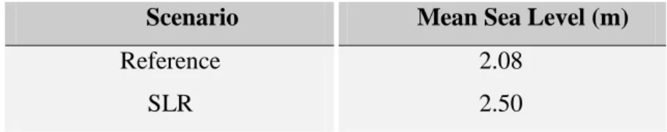
4.2. Impact of sea level rise

The main goal of studying the sea level rise in this context was to research the biological response of the Tagus Estuary to sea level rise, once it is a serious consequence of climate change due to its impact in society and ecosystems (Lopes et al., 2011; Valentim et al., 2013). Analysis of tide-gauge data have indicated a global sea level rise (SLR) during the 20th century and several studies predict that it is going to continue during 21st century, increasing coastal hazards (Lopes et al., 2011). In order to study this issue, two scenarios were set (Table 5). One reference scenario with the actual mean sea level value, and the initial and boundary conditions for March of 2004, and other considering a SLR of 0.42 m, predicted by Lopes et al. (2011). Notwithstanding, the magnitude of sea

(48)

level rise remains controversial among the scientific community and projections still present a large uncertainty (Guerreiro et al., 2015). It is noteworthy that the

Table 5: Scenarios description for Sea Level Rise.

Scenario Mean Sea Level (m)

Reference SLR

2.08 2.50

last IPCC report, suggests a global mean SLR by the year 2100 that vary between 0.26 and 0.98 m (Guerreiro et al., 2015).

Both simulations were performed for 31 days to evaluate Chl-a and nutrient concentration (nitrate and phosphate) distribution along the tidal cycle (spring and neap tide) for four instants: low tide, flood, high tide and ebb periods. The reference situation is characterized for spring tide (Figure 10) and neap tide (Figure 12), and then it is compared with the results that consider a SLR of 0.42 m (Figures 11 and 13). For instant A (Figure 10 – top panel A), which corresponds to the high tide, the Chl-a concentration is high on the lower estuary, reaching values up to 0.4 mg m-3, decreasing gradually upstream, reaching 0.3 mg m-3 on the middle estuary and 0.2 mg m-3 on the upper estuary. When the SLR scenario is considered (Figure 11 – top panel A), it is observed a decrease relative to reference of the Chl-a concentration in the estuary mouth channel and in the upper estuary of approximately 0.020 mg m-3. Otherwise, an increase of approximately 0.025 mg m-3 is observed in the middle estuary, which represents an increase of 8%.

Regarding the reference scenario, from the high tide instant (A) to the ebb instant (B) Chl-a concentration is slightly higher in the mouth channel and lower in the middle estuary (0.4 mg m-3 in the mouth channel and 0.45 mg m-3 in the middle estuary), suggesting that the rich phytoplankton water is being transported towards the estuary mouth. This trend is still observed from instant B to C.

Comparing the results of the SLR scenario with the reference, for instant B (Figure 10 – top panel) the Chl-a concentration slightly increases (4%), on the middle estuary and decrease in the estuary mouth and upper estuary (8%). For the low tide instant (C), the results show that in the upper estuary, differences between the Chl-a concentration for SLR scenario and reference are negative, which means that the concentration considering an