Inputs and yield optimization on irrigated
maize
Otimização da produtividade e dos fatores de produção no milho de
regadio
Anabela Dias Ramalho Vale Leitão Grifo
Tese apresentada à Universidade de Évora para obtenção do Grau de Doutor em Ciências Agrárias na especialidade Agronomia
Orientadores José Rafael Marques da Silva Maria Manuela Melo Oliveira Carlos Alberto de Jesus Alexandre
Évora, setembro de 2015
UNIVERSIDADE DE ÉVORA
Escola de Ciências e Tecnologia Departamento de Fitotecnia
Inputs and yield optimization on irrigated maize
Anabela Dias Ramalho Vale Leitão Grifo
Orientação José Rafael Marques da Silva Maria Manuela Melo Oliveira Carlos Alberto de Jesus Alexandre
Ciências Agrárias Dissertação
“Everything is related to everything else, but near things are more related than distant things.” Waldo Tobler, 1979
Acknowledgements/Agradecimentos
No final deste trabalho gostaria de testemunhar o meu agradecimento a diversas pessoas e instituições que, direta ou indiretamente, contribuíram de forma significativa para sua realização.
Ao meu orientador, Professor Doutor José Rafael Marques da Silva, pela excelente orientação científica, incan-sável ajuda e apoio em todas as tarefas e fases do trabalho. Obrigada pelos seus ensinamentos, pela dinâmica de trabalho e constante estímulo e pela sua pronta e inesgotável disponibilidade. Não posso ainda deixar de referir a sua enorme paciência e compreensão, entusiasmo, simpatia e amizade demonstrada ao longo destes anos e que foram decisivos para ultrapassar algumas situações difíceis. Mesmo nos momentos mais complica-dos fez-me sempre acreditar que era possível.
Aos meus coorientadores científicos, Professora Doutora Maria Manuela Melo Oliveira e Professor Doutor Car-los Alberto de Jesus Alexandre pela orientação, incentivo, esclarecimentos e sugestões, confiança, enorme disponibilidade e simpatia com que sempre me receberam. Há momentos que fazem a diferença.
Ao Professor Doutor Gottlieb, director do curso de doutoramento em Ciências Agrárias da Escola de Ciência e Tecnologia da Universidade de Évora pelo acolhimento no curso de doutoramento.
Ao Instituto de Ciências Agrárias e Ambientais Mediterrânicas (ICAAM) por ter sido a minha unidade de acolhi-mento durante a realização da investigação desenvolvida nesta dissertação.
Ao Engenheiro Castro Duarte e seus colaboradores por todas as condições que me proporcionaram para de-senvolver o trabalho de campo.
À Escola Superior Agrária de Santarém (ESAS) e em particular ao Professor Coordenador José Mira de Villas Boas Potes, diretor da ESAS, ao Professor Coordenador António do Patrocínio Amaral de Azevedo, na qualidade de ex-diretor da ESAS, ao Professor Coordenador Manuel Mendes de Sousa Adaixo, presidente do Departamento de Ciências Agrárias e Ambiente da ESAS e ao Professor Adjunto António Mendes Marques, presidente da Unidade Laboratorial de Ciências Agrárias e Ambiente da ESAS, pela amizade, entusiasmo e por me proporcionarem total liberdade em utilizar a Unidade Laboratorial de Ciências Agrárias e Ambiente.
Ao meu marido, Luís Grifo, um dos pilares da minha vida, por acreditar em mim mais do que eu própria, e ser sempre a minha estrutura de apoio de forma incondicional. Trabalhou de forma incansável na recolha de dados de campo, muitas vezes em condições adversas e sempre com alegria e boa disposição. Conseguiu transformar momentos complicados em momentos felizes. É a minha fonte de força que me incutiu a determinação em querer chegar mais longe.
À Mestre Albertina Ferreira, colega de trabalho e grande amiga, que me acompanhou ao longo de todo este per-curso, me auxiliou em muitos momentos e com quem partilhei algumas lágrimas mas também muitas garga-lhadas e muitas horas de trabalho tornando este trajeto muito mais ameno. Emocionalmente, a boa disposição que partilhámos foi relevante para a realização deste estudo.
À minha irmã, Esmeralda Cristina que, com o seu amor incondicional, me fez a revisão dos textos em inglês, muitas vezes com prejuízo próprio. O seu apoio, carinho e compreensão foram essenciais para tornar os meus dias mais harmoniosos.
Às colegas e amigas, Professora Adjunta Ana Claúdia Charana e Professora Adjunta Ana Ambrósio Paulo que me apoiaram em termos de serviço letivo, ouviram os meus lamentos e me proporcionaram bom ambiente de trabalho e um alegre convívio.
À Mestre Maria Fernanda Rebelo, colega e grande amiga, pelo entusiasmo e preciosa ajuda na determinação, coordenação e orientação de todas as análises de solos. À equipa de funcionários da Unidade Laboratorial de Ciências Agrárias e Ambiente da ESAS (Rute Sales Costa, José Manuel Saragoça, Maria Madalena Mascarenhas e Maria José Maia) e às alunas Ana Catarina Rebelo e Ana Rita Pereira que disponibilizaram o seu tempo para colaborar amavelmente na realização de algumas tarefas, revelando sempre boa disposição.
Ao Laboratório Químico Agrícola (LQA) da Universidade de Évora pela ajuda na determinação de alguns parâme-tros do solo.
Ao meu colega e amigo Mestre Rodrigo Rodrigues que com amabilidade que o carateriza me acompanhou e ajudou em alguns trabalhos de campo.
Ao jovem, Luís Marques da Silva que ajudou na recolha de dados de campo com energia e entusiasmo. Aos meus queridos filhos, Eduardo Grifo e Bruno Grifo pelo seu carinho e amor e por compreenderem as i-númeras ausências. Trabalharam de forma incansável na recolha de dados de campo mostrando sempre com-preensão e entusiamo mesmo em condições hostis. Que este trabalho lhes sirva de motivação e exemplo de que vale sempre a pena investirmos em nós próprios e em novos desafios, independentemente da nossa idade. Aos meus pais, Maria Celeste e António Leitão, pelo seu amor sem dimensão, pelos princípios e valores que me incutiram, por me “mimarem” durante toda a vida, por estarem presentes de forma incondicional nos momen-tos mais difíceis, por me ensinarem a importância dos “estudos” e acreditarem em mim.
À minha família, especialmente sogros, cunhados e sobrinhos por compreenderem o meu afastamento e ausên-cias e por toda a alegria e carinho que me proporcionaram.
Aos meus amigos, Lígia Coelho, Alexandre Coelho e Dra. Maria Pilar Rosinha pela boa disposição, incentivo, amizade e disponibilidade com os meus filhos, dando o apoio necessário sempre que lhes solicitava.
Às minhas amigas Doutora Maria Encarnação Marcelo, Mestre Iris Crispim, Doutora Rita Neres, Doutora Marta Madeira, Professora Adjunta Maria Adelaide Oliveira, Doutora Ana Mafalda Ferreira, Professora Adjunta Paula Lúcia Ruivo, Professora adjunta Rosa Santos Coelho, Especialista José Manuel Carvalho, Professora Adjunta Helena Mira que em muitos dos momentos mais sensíveis me ouviram, compreenderam e incentivaram. A todos os colegas e funcionários da ESAS e amigos que tiveram sempre uma palavra de estímulo.
Ao Professor Doutor Francisco Coelho pelo trabalho e disponibilidade em adequar o “template do latex” à si-tuação desta dissertação.
A todos
Contents
Contents xi
List of Figures xv
List of Tables xvii
Acronyms xix Abstract xxi Sumário xxiii 1 Introduction 1 1.1 Objectives . . . 2 2 Scientific background 3 2.1 Precision agriculture . . . 3
2.2 Spatial and temporal variability . . . 4
2.2.1 Yield . . . 4 2.2.2 Soil . . . 5 2.2.3 Topography . . . 6 2.2.4 Other sources . . . 7 2.3 Management zones . . . 7 2.4 Evaluating variability . . . 8 2.4.1 Grid sampling . . . 8 2.4.2 Sensors . . . 9 2.5 Variable-rate technology . . . 12 xi
3 Exploratory Field Risk Analysis Considering Space and Multi-Year Maize Yield 13
3.1 Introduction . . . 14
3.2 Materials and Methods . . . 15
3.2.1 Collecting and processing yield data . . . 15
3.2.2 Data analysis . . . 16
3.3 Results . . . 18
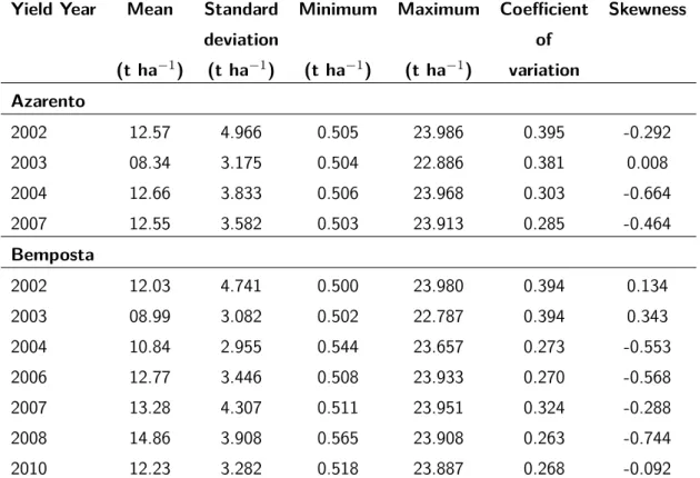
3.3.1 Grain yield descriptive statistics . . . 18
3.3.2 Grain yield spatial dependence . . . 19
3.3.3 Principal Components Analysis . . . 19
3.4 Discussion . . . 21
3.5 Conclusions . . . 28
4 Stochastic simulation of maize productivity: spatial and temporal uncertainty in order to manage crop risks 29 4.1 Introduction . . . 30
4.2 Materials and Methods . . . 31
4.2.1 Details of the field experimental site and the collection of yield data . . . 31
4.2.2 Data processing and analysis . . . 32
4.3 Results and Discussion . . . 33
4.3.1 Exploratory and spatial structure analyses . . . 33
4.3.2 Real Yield Data . . . 36
4.3.3 Yield Stochastic Simulations . . . 36
4.3.4 Yield classes and their occurrence probability . . . 50
4.4 Conclusions . . . 51
5 Maize fertilization: soil phosphorous and potassium optimization - yield/input ratio 53 5.1 Introduction . . . 54
5.2 Materials and methods . . . 56
5.2.1 Study field . . . 56
5.2.2 Digital elevation model . . . 56
5.2.3 Apparent soil electrical conductivity measurements (ECasurvey) . . . 56
5.2.4 Soil sampling and laboratory procedures . . . 57
5.2.5 Data analysis . . . 57
5.2.6 Yield/input ratio . . . 60
5.2.7 Crop budget . . . 60
5.3 Results . . . 60
CONTENTS xiii
5.3.2 Yield/nutrient input ratio of phosphorus and potassium . . . 63
5.4 Discussion . . . 66
5.4.1 Differential fertilization - decision making . . . 66
5.4.2 Differential fertilization - economic aspects . . . 67
5.5 Conclusions . . . 69
6 General Discussion, Future Work and Conclusions 71 6.1 General discussion . . . 71
6.2 Future work . . . 73
6.3 Conclusions . . . 74
A Figures 77
B Maize production costs 87
List of Figures
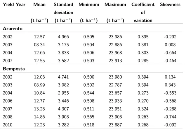
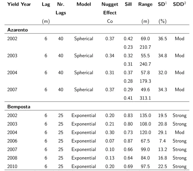
3.1 (a) 2002 yield variogram for the Azarento field; (b) 2006 yield variogram for the Bemposta field. . 19 3.2 Standardized maize yield maps for the Azarento field: (a) yield in 2002; (b) yield in 2003; (c) yield
in 2004; (d) yield in 2007. . . 22 3.3 Azarento field: (a) temporal yield standard deviation; (b) average temporal maize yield; c) first
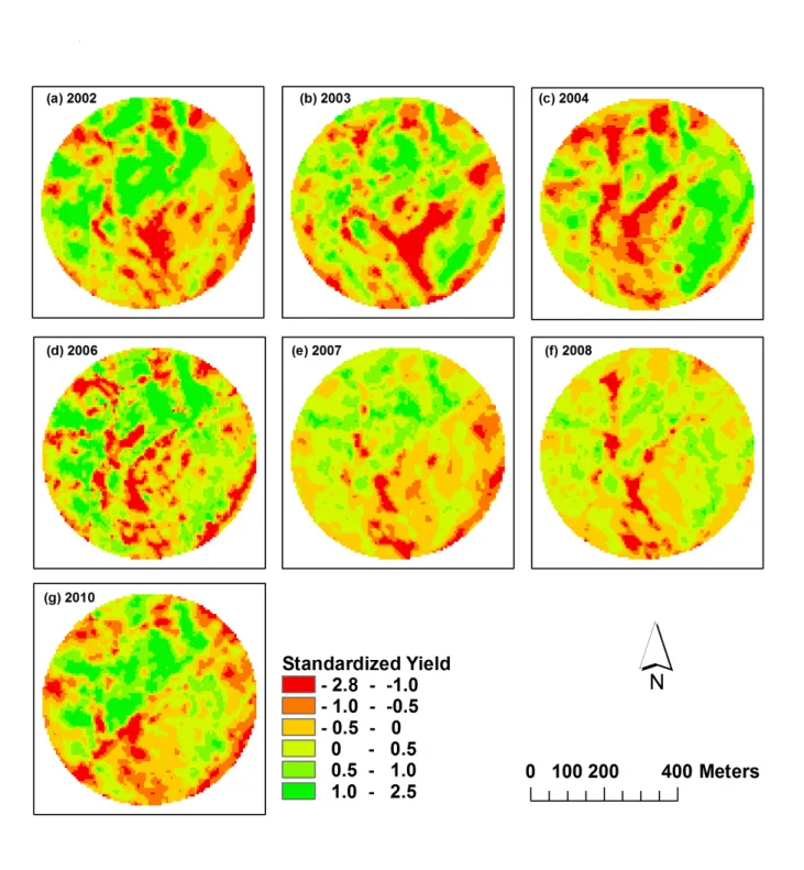
principal component scores; (d) second principal component scores. . . 23 3.4 Standardized maize yield maps for the Bemposta field: (a) yield in 2002; (b) yield in 2003; (c)
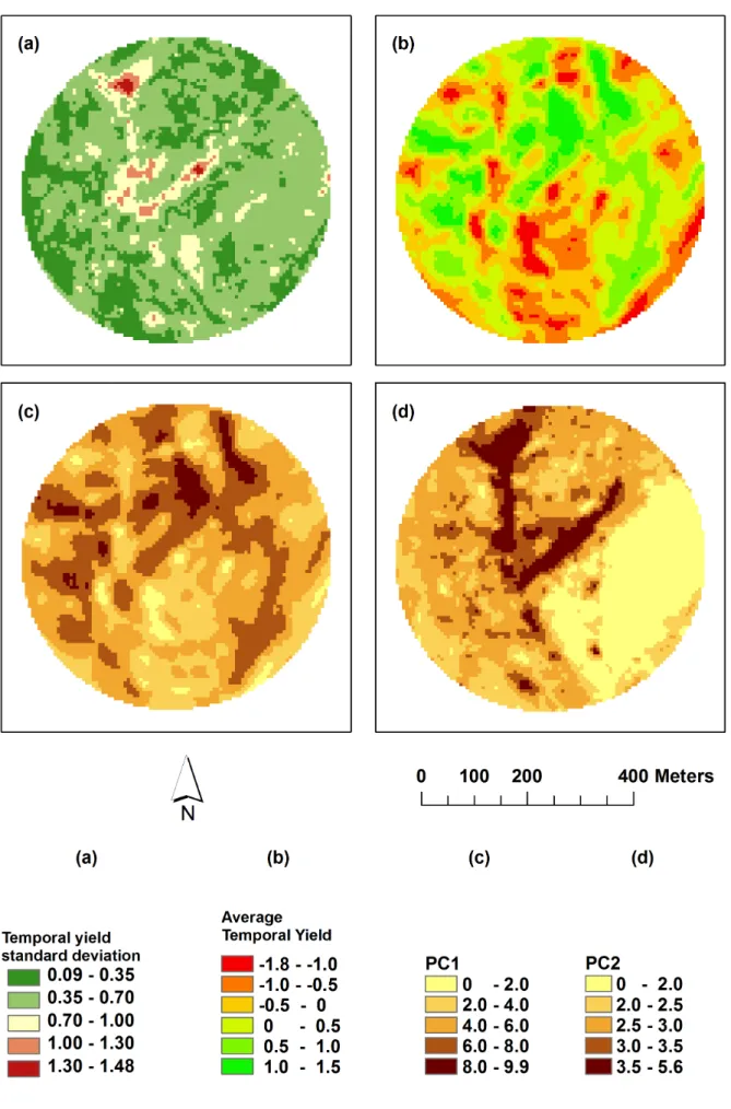
yield in 2004; (d) yield in 2006; (e) yield n 2007; (f) yield in 2008; (g) yield in 2010. . . 24 3.5 Bemposta field: (a) Temporal yield standard deviation; (b) Average temporal maize yield; (c)
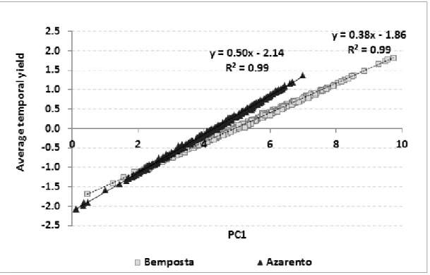
First principal component scores; (d) Second principal component scores. . . 25 3.6 Plot of the first principal component scores (PC1) vs. the average temporal yield of 300 random
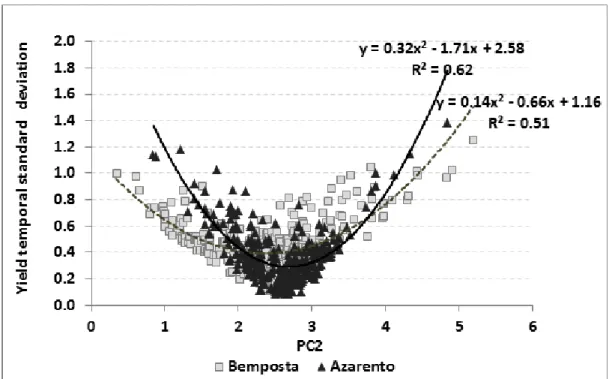
yield observations in the Azarento and Bemposta fields. . . 26 3.7 Plot of the second principal component scores (PC2) vs. the temporal yield standard deviation
for 300 random yield observations in the Azarento and Bemposta fields. . . 27
4.1 Maize yield variogram - 2002. . . 34 4.2 Field area percentage according to different standard yield classes and different initial point
densities for stochastic simulation: (a) Azarento field; (b) Bemposta field. . . 42 4.3 Real and simulated yield (≈ 65% points ha−1) field area percentage according to different
stan-dard yield classes (Azarento field): (a) 2002; (b) 2003; (c) 2004; (d) 2007. . . 43 4.4 Average real yield and simulated yield (≈ 65% points ha−1) field area percentage according to
different standard yield classes and considering 4 years (Azarento field). . . 44 4.5 Below-average yield areas with 80% confidence considering 2002, 2003, 2004 and 2007
simula-tion data analyzed independently (Azarento field). . . 47 4.6 Above average yield areas with 80% confidence considering 2002, 2003, 2004 and 2007
simula-tion data analyzed independently (Azarento field). . . 48 4.7 Below-average (a) and above-average (b) yield areas with 80% confidence considering 2002,
2003, 2004 and 2007 simulation yield data grouped together (Azarento field). . . 49
5.1 (a) Digital elevation model (DEM): contour, slope and soil sampling points; (b) ECaspatial distri-butionm. . . 58 5.2 Maize yield spatial statistics: (a) yield average and (b) yield standard deviation. . . 61 5.3 The soil (a) phosphorus and (b) potassium spatial distribution. . . 62 5.4 Spatial distribution of the yield/input ratio of (a) phosphorus (Pyr) and (b) potassium ((Kyr). . . 63 5.5 Yield/phosphorus ratio zones (Z1, Z2, Z3, Z4 and Z5) according the 2007 maize yield; (Y+ higher
yield; Y- lower yield; P+ higher phosphorus soil concentration; P- lower phosphorus soil concen-tration). . . 64 5.6 One-to-one straight line comparison between yield/phosphorus racio (Pyr) and yield/potassium
racio ((Kyr). . . 67 5.7 Management zones (Z1, Z2, Z3, Z4 and Z5) according to the 2007 maize yield and yield/input
ratio of 0.12 t ha−1(mg Kg−1)−1. . . 68
A.1 DEMs for: (a) Azarento field; b) Bemposta field. . . 78 A.2 Real and simulated yield (≈ 65 points ha−1) field area percentage according to different
stan-dard yield classes Bemposta field: (a) 2002; (b) 2003; (c) 2004; (d) 2006. . . 79 A.3 Real and simulated yield (≈ 65 points ha−1) field area percentage according to different
stan-dard yield classes Bemposta field: (e) 2007; (f) 2008; (g) 2010. . . 80 A.4 Average real yield and simulated yield (≈ 65 points ha−1) field area percentage according to
different standard yield classes and considering 7 years (Bemposta field). . . 81 A.5 Below average yield areas with 80% of confidence considering 2002, 2003, 2004 and 2006,
sim-ulation data analyzed independently (Bemposta field) . . . 82 A.6 Below average yield areas with 80% of confidence considering 2007, 2008 and 2010 simulation
data analyzed independently (Bemposta field) . . . 83 A.7 Above average yield areas with 80% of confidence considering 2002, 2003, 2004 and 2006
sim-ulation data analyzed independently (Bemposta field). . . 84 A.8 Above average yield areas with 80% of confidence considering 2007, 2008 and 2010 simulation
data analyzed independently (Bemposta field). . . 85 A.9 Below average (a) and above average (b) yield areas with 80% of confidence considering 2002,
List of Tables
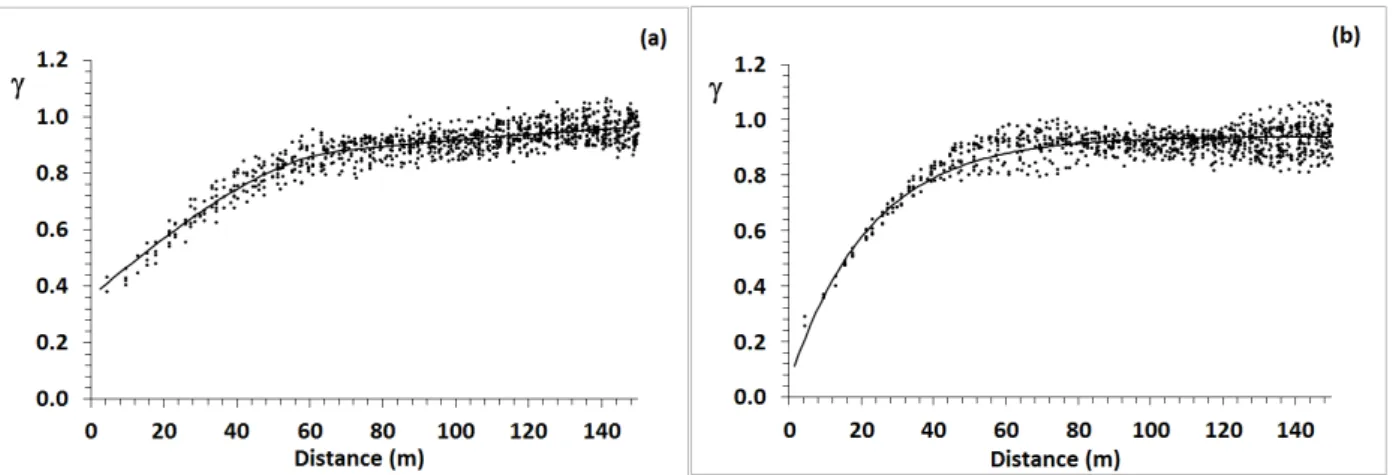
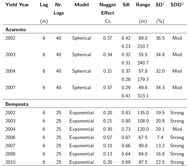
3.1 Summary statistics for grain yield at the Azarento and Bemposta agricultural fields. . . 18 3.2 Maize yield data variogram parameters for Azarento (2 structures) and Bemposta agricultural
fields. . . 20 3.3 Values of the eigenvector loadings for each variable and percentage of explained variance by
the first two axes for Bemposta and Azarento fields. . . 21
4.1 Summary statistics for grain yield in Azarento and Bemposta agricultural fields. . . 34 4.2 Maize yield data variogram parameters for Azarento (2 structures) and Bemposta agricultural
fields. . . 35 4.3 Percentages of yield standard classes for real yield in the Azarento field. . . 36 4.4 Percentages of yield standard classes for real yield in the Bemposta field. . . 37 4.5 Percentages of yield standard classes for the 2002 simulated yield data in the Azarento field
considering 30, 65, 125 and 200 points ha−1of yield data positions randomly. . . 38 4.6 Percentages of yield standard classes for the 2002 simulated yield data in the Bemposta field
considering 30, 65, 125 and 200 points ha−1of yield data positions randomly. . . 38 4.7 Percentages of the yield standard classes for simulated yield data in the Azarento field
consid-ering 65 points ha−1of yield data positions for 2002, 2003, 2004 and 2007. . . 39 4.8 Percentages of yield standard classes for simulated yield data in the Bemposta field considering
65 points ha−1of yield data positions for 2002, 2003, 2004, 2006, 2007, 2008 and 2010. . . 40 4.9 Percentage differences between real yield and yield simulation classes considering ≈ 65%
points ha−1of yield data positions (Azarento). . . 41 4.10 Percentage differences between real yield and yield simulation classes considering≈ 65%
points ha−1of yield data positions (Bemposta). . . 41 4.11 Percentage differences of minimum, maximum and average yield values per yield class between
real yield data and simulated yield data, considering≈ 65% points ha−1of yield data. . . 44 4.12 Field area percentage below the yield average according to 95%, 90%, 80%, 70%, 60% and 50%
confidence levels, considering yield simulations from≈ 65% points ha−1of real yield data. . . 45 xvii
4.13 Field area percentageabove-yield average according to 95%, 90%, 80%, 70%, 60% and 50%
con-fidence levels, considering yield simulations from≈ 65% points ha−1of real yield data. . . 46
5.1 Phosphorus, potassium, apparent soil electrical conductivity and yield of 2007 data variogram parameters. . . 59
5.2 Grain yield summary statistics for the Azarento field. . . 61
5.3 Soil P levels and yield/P racio according to Z1, Z2, Z3, Z4 and Z5 zones. . . 65
5.4 Soil K levels and yield/K racio according to Z1, Z2, Z3, Z4 and Z5 zones. . . 66
5.5 Fertilization scenarios. . . 70
5.6 Fertilizer units applied in each scenario. . . 70
Acronyms
CEC Cation exchange capacity DEM Digital elevation model
DGNSS Differential Global Navigation Satellite System Ca Calcium
CEC Cation exchange capacity ECa Apparent electrical conductivity EMI Electromagnetic Induction ER Electrical resistivity method GIS Geographic Information Systems GNSS Global Navigation Satellite System K Potassium
Mg Magnesium N Nitrogen
NDVI Normalized difference vegetation index PA Precision agriculture
OM Organic matter P Phosphorous
PCA Principal component analysis PC1 1stprincipal componente PC2 2ndprincipal componente SGS Sequential Gaussian Simulation VRA Variable rate application VRT Variable rate technology
Abstract
This dissertation describes efforts to move toward the study of soil and the management of yield variability through research that explored and evaluated the potential of some techniques to provide greater under-standing and knowledge of an agricultural field, even in situations where there is no prior knowledge of its behavior. The first experiment used a principal components analysis (PCA) in the study of the spatial and temporal variability of maize grain yield. The results of this experiment demonstrated that the 1stand 2nd principal components could be used to identify field zones with different spatial and temporal behaviors. The second experiment applied stochastic and sequential Gaussian simulation techniques to spatially and temporally forecast and model maize productivity. This technique enabled the modeling of spatial uncer-tainty in maize productivity based on probabilistic maps with different confidence levels. The third exper-iment examined different fertilization input scenarios based on yield/nutrient inputs ratio and break-even yields to optimize agronomic, economic and environmental support decisions. According to the results, it is possible to reduce agricultural production costs through the differential management of inputs. The outcomes showed that differential management decisions can maximize returns and reduce activity risk without having to implement major changes on the farm.
Keywords: maize yield; yield principal components analysis; yield stochastic simulation; differential inputs dis-tribution; management zones
Sumário
Otimização da produtividade e dos fatores de produção no milho de regadio
O presente trabalho de investigação, que considerou três estudos, explora e avalia o potencial de alguns modelos no estudo da gestão da variabilidade espacial e temporal da produtividade e dos nutrientes no âmbito da produção de regadio. O primeiro estudo focou a utilização da técnica estatística Análise de Com-ponentes Principais (ACP) no estudo da variabilidade temporal da produtividade da cultura do milho na região do Alto Alentejo. Os resultados desta experiência mostraram que as duas primeiras componentes principais permitem identificar zonas da parcela agrícola com diferente comportamento espacial e am-biental. No segundo estudo avaliou-se o desempenho da simulação sequencial Gaussiana na previsão e modelação da produtividade da cultura do milho. Esta técnica permitiu modelar a incerteza espacial da produtividade com base em mapas de probabilidade com diferentes níveis de confiança. O terceiro es-tudo avaliou diferentes cenários de fertilização a partir do rácio produtividade/nutrientes e do breakeven da produtividade de forma a otimizar, em termos agronómicos, económicos e ambientais, as tomadas de decisão. De acordo com os resultados obtidos, foi possível obter uma redução substancial dos custos de produção através da sugestão da aplicação diferenciada da fertilização. Os resultados mostraram que é possível reduzir os riscos, quer económicos quer ambientais, da atividade agrícola sem grandes alterações no processo produtivo da exploração agrícola.
Palavras-chave: produtividade da cultura milho, análise de componentes principais, simulação estocástica, fertilização diferenciada, zonas de gestão localizada
1
Introduction
To produce more food and reduce economic and environmental costs, agricultural activities need to combine smart technologies with smart agro-processes. Traditional farming considers the management of agronomic fields to be uniform despite the spatial variability that can be found within a field. Precision agriculture accounts for the spatial variability of fields and promotes site-specific management to increase economic returns and minimize environmental impacts [BBSM07, MTM10].
In Portugal, little research has been done on the delineation of management zones, and there is a general lack of literature on this subject. However, some researchers have developed studies of variable rate pasture appli-cations (e.g., [PSM+05, SSMds14]), spatial yield variability (e.g., [Mar06, MRSM12]), topography (e.g., [MA05]) and
soil mechanical resistance (e.g., [CaEF+12]).
Every day, agriculture is confronted with numerous challenges, so the adoption of modern technology by global agriculture is inevitable, and Portugal is not an exception. In the future, agriculture will be severely competitive and challenging, and all of the available tools, technology and knowledge will be necessary to sustainably in-tensify this activity.
Geographic information systems and geostatistical tools can be used to develop thematic maps of soils, yields and other parameters, which are extremely important for spatially and temporally efficient agricultural ma-nagement.
The accurate mapping of yield-limiting factors remains a challenge for researchers [CC08]. Topographic at-tributes, soil properties and climate constraints interact to influence the spatial and temporal variability in yields. However, this variability is not an independent phenomenon; it reflects within-field variation of the soil yield potential [PJABa06] and can be an important factor for the delineation of within-field management zones [Bla00, FWWB00, Mar06].
Applying site-specific practices will improve net returns and minimize environmental impacts [LWHT10, SPdS+10,
SSS14]. In other words, modern agriculture is technologically demanding, so there is a need for more research, and farm managers must exercise best practices to achieve yield and environmental targets.
1.1 Objectives
The purpose of this work is to explore several useful strategies that have been developed to assess the spatial and temporal variability in yield. These strategies are intended to improve future agronomical prescriptions and allow for a more accurate estimation of variable rate management to reduce risks and enhance environmental and economic benefits.
This dissertation is divided into three parts:
i) The first part (Chapter 2) is an introduction to the problems addressed in the manuscripts on which this thesis is based, and it provides an overview of the theoretical foundation of the dissertation;
ii) The second part (Chapters 3, 4, 5) is comprised of three scientific manuscripts that have already been pub-lished or submitted for publication in international peer-reviewed journals, and they were developed to answer several research questions:
• a) Chapter 3 describes how the multivariate principal components analysis technique can be simulta-neously used to delineate yield management zones and to identify specific locations inside a field with temporal yield resilience, i.e., to calculate the temporal risk associated with maize yield;
• b) Chapter 4 explores the possibility of using stochastic simulation techniques to forecast maize produc-tivity and model spatial and temporal uncertainty using probabilistic yield maps when there is a lack of data;
• c) Finally, Chapter 5 presents a yield/input ratio approach and yield break-even as potential tools to help farmers and managers 1) optimize agronomic inputs, 2) delineate management zones, and 3) reduce economic and environmental risks from production;
iii) The third part (Chapter 6) integrates all of the scientific discussions and conclusions presented in this docu-ment and considers the implications for further research.
2
Scientific background
2.1
Precision agriculture
Precision agriculture (PA) is also known as precision farming or site-specific crop management. The term first appeared in 1990 as the title of a workshop in Great Falls, Montana, which was sponsored by Montana State Uni-versity, but researchers had previously used the terms “site-specific crop management” or “site-specific agricul-ture” [Oli10].
There are many definitions for precision agriculture (PA), but all of them describe a crop production system with low inputs and high efficiency as well as environmental and economic benefits.
According to Schellberg et al. [SHG+08], PA is “an innovative, integrated and internationally standardized
ap-proach that aims to increase the efficiency of resource use and to reduce the uncertainty of decisions required to control variation on farms”.
Another example is the more detailed definition by Sudduth [Sud99], who defined PA as “a management sys-tem of crop production practices and inputs such as seed, fertilizers and pesticides that are variably applied within a field. Input rates are based on the needs for optimum production at each within-field location. Since
over-application and under-application of agrochemicals are both minimized, this strategy has the potential for maximizing profitability and minimizing environmental impacts”.
In fact, PA is as old as agriculture itself. In the early days, each farmer knew each portion of his land well and cul-tivated and devoted his attention to fields based on their characteristics, thus ensuring enough food to sustain his family. However, in recent decades, the need to produce more food and the growth of cultivated areas has led farmers to treat fields as homogeneous zones, so management is based on the average needs for fertilizer, water and pesticide inputs. For a long time, site-specific crop management was ignored.
The adoption of PA gradually occurred over many years, but PA is currently a fact thanks to a set of technologies such as Global Navigation Satellite Systems (GNSS), geographic information systems (GIS), remote sensing, sen-sors and data-acquisition systems, computer science, simulation models, agricultural machinery, and variable rate application systems (VRT), as well as the interest of humans in better practices .
The spatial and temporal variability of soil and crop factors are the basis for PA [ZWW02]. Spatial variability refers to how soil properties and production vary in space. Temporal variation is a major source of production risk because it is difficult to control; it occurs over years due to weather or seasonal events [Toz09]. However, the power of new technologies in the collection, storage, processing and display of spatial data makes it possible to obtain comprehensive information about yield variability in space and time [ZWW02].
However, the way forward is not to present PA as a solution for all or to impose the system on farmers but to assist them and share information so that they can put questions to PA experts.
As reported by Schellberg et al. [SHG+08], “the key to successful future PA is not only to collect relevant data but
also to convert them into useful information and then derive consequential decisions and rigorously evaluate risks and benefits”.
2.2
Spatial and temporal variability
The spatial and temporal variability of the soil, yield and crop attributes are the basis for PA, and several ap-proaches can be used to study yield variability. It is challenging to identify and comprehend spatial and tem-poral variability because there are many parameters involved in the production process. Therefore, some au-thors consider the spatial and temporal variability of different factors, such as yield variability, crop variability, field variability, soil variability, variability in anomalous factors, and management variability [ZWW02]. Other re-searchers incorporate different types of data sets to define zones with more or less uniform production potential [KZN+14].
2.2.1 Yield
The goal of the spatial and temporal analysis of yield variability is to delineate areas with consistent yield pat-terns to develop practices that can optimize crop production.
The availability of yield monitors equipped with GNSS, which can generate spatially dense data at relatively low cost, has stimulated the study of spatial and temporal yield variability and interest in the site-specific ap-plication of crop inputs [LCD99]. This simple method of data collection has encouraged several researchers to analyze yield variability over space and time. Diker et al. [DHB04] showed that spatial and temporal yield can be analyzed with multi-year data to detect broad patterns that are preserved over time. With only a few years of yield data, a farmer or manager can try to identify the yield-limiting factors in similar and dissimilar zones. If possible, the farmer should amend the problem in the subsequent years of production, but the causes of
vari-2.2. SPATIAL AND TEMPORAL VARIABILITY 5
ability can change with time and the type of crop [VPG03]. As evidenced by Blackmore at al. [BGF03], temporal variability is generally much higher than spatial variability, so care must be taken when defining areas of low and high productivity as potential zones for site-specific management.
According to Diacono et al. [DCT+12], when crops grow in a rain-fed Mediterranean environment, the different
spatial yield distributions from one cropping season to another may be mainly due to the influence of meteo-rological conditions. This conclusion is in agreement with other results, such as those of Link et al. [LGC04] in Germany, who found that maize grain yield was affected by climatic variations from year to year over six years, or those of Basso et al. [BCC+09], who concluded that soil water content was the main factor affecting spatial
variability in yield.
When a temporal trend in yield is identified in a given part of a field over multiple years, its effect can be cal-culated, and Blackmore et al. [BGF03] and Marques da Silva [Mar06] proposed a modified standard deviation function to quantify this variance. This function was able to detect spatial changes over time, e.g., parts of a field where yield is always close to the mean (low temporal variance) and parts that are temporally unstable because they sometimes produce above-average yields but produce below-average yields at other times (high temporal variance). Consequently, Blackmore et al. [BGF03] and Marques da Silva [Mar06] divided their tem-poral variance and spatial variability maps into four homogeneous classes: (1) high yielding areas – zones in which the yield is above the inter-annual mean; (2) low yielding areas – zones in which the yield is below the inter-annual mean; (3) stable areas – zones with low inter-annual spatial variance (based on an arbitrarily de-fined threshold) and (4) unstable areas – zones with high inter-annual spatial variance (based on an arbitrarily defined threshold).
The analysis of different patterns of yield in space and time can be further applied to the analysis of other factors, such as crop density, crop height, crop nutrient stress, crop water stress, crop biophysical properties, crop leaf chlorophyll content, and crop grain quality [ZWW02, DMV07]. Crop models can be used to better understand the effects of these factors, which are directly related to the plants, and the processes involved in crop growth and thus identify the spatial and temporal variability in yield. The study of the daily growth of crops under a few stresses, such as water, nitrogen (N), temperature or pests, with different models has been used to identify the causes of spatial variability in yield [BBP02].
In Italy, Basso et al. [BBSM07] studied the growth of corn, soybeans and wheat (under crop rotation) using models that simulate the responses of crop growth and development to different environmental conditions. These models incorporate different types of information, such as soil data (sand, silt and clay content, bulk density, organic carbon and water limits), the standard deviations of temporal yield data calculated according to Blackmore [Bla00] and Blackmore et al. [BGF03], weather data (incoming solar radiation, air temperature and rainfall), and yield data from yield monitoring systems during different growing seasons. The models were applied to two areas identified as stable, i.e., with higher or lower than average yields and lower temporal vari-ance over time. The difference between the annual simulated and measured yield data was acceptable, but the long-term simulated yield data varied for all crops, which confirmed the influence of climatic data and soil properties on the average yield [BBSM07].
2.2.2 Soil
The spatial variability of crop production reflects the variability in soil fertility, which depends on physical and chemical soil properties [AHMU04, PGZ+07].
Although the geological and pedological processes of soil formation determine the spatial variability in the soil, some physical soil properties can be altered over time due to soil erosion and management practices, such as tillage [ITJ+05, VVS+08]. For example, Iqbal et al. [ITJ+05] identified the higher soil bulk density in subsurface
horizons, which restricts downward water movement, as perhaps being due to the compaction of fine sandy or fine silt layers by heavy machinery.
In 2005, a study of the spatial variability of the physical soil properties of three fields over three years became important to the delineation of different zones with distinct maize yield potentials. Soil properties were re-latively homogeneous inside each zone but were significantly different between zones, so the available water, and thus nutrient uptake, may have differed from zone to zone, reflecting the potential productivity of each area [MKR+05]. Cox et al. [CGWA03] and Guo et al. [GMB12] made similar observations and found that the clay
content was an adequate criterion for dividing fields into areas of equal productivity. These authors suggested that the higher yield in areas with higher clay content is related to the availability of more plant-available water during the dry periods of the growing season [CGWA03, GMB12] because soil texture is one of the most important factors influencing the water-holding capacity of the soil [SSL+04, GMB12].
In addition to the physical soil properties, other researchers have studied chemical properties and/or nutrient status to better understand the variability in yield across fields. Ping et al. [PGZ+07] found low temporal
variabi-lity in pH, cation exchange capacity (CEC), calcium (Ca) and texture over time, and other studies [KB00, LGC04] have found that soil properties, such as organic matter (OM), pH, phosphorous (P), potassium (K), magnesium (Mg) and nitrogen content do not directly explain the spatial variability in yield. In fact, the nutrient response patterns within a field often do not mimic yield patterns, which implies that there are other factors, such as topographic attributes, that affect crop yields [KB00, LGC04].
2.2.3 Topography
Actually, some researches have shown that, in general, the spatial variabilities in soil and yield are very closely associated with their position on the landscape. For instance, Aimrun et al. [AAR+09] studied the distribution
of several chemical soil properties, and the lowest positions in the study area exhibited high total N, available P, exchangeable K, Ca, Mg and total organic carbon values compared with the highest positions, which is probably due to the dynamics of surface runoff water.
Guo et al. [GMB12] found that topography, combined with other factors, explained up to 70.1% of the variability in cotton yield, which agrees with the results of Kaspar et al. [KCJ+03], who, in a study over four dry years in
Iowa, found that topography explained 78% of the spatial variability in maize yield due to the effects of soil properties, soil erosion and water availability.
Curvature is an important topographic factor that determines the movement of water and nutrients in the soil, and the influence of the curvature profile on yield is more obvious in dry years than in wet years [KKKM11, KZN+14]. Usually, a convex curvature is associated with soil erosion, and a concave curvature is associated
with soil, water and nutrient deposition [GMB12]. Although this does not always happen, concave areas should theoretically have greater water and nutrient availability and thus be more productive [KB02, SSL+04, BCC+09,
GMB12].
This conclusion is supported by the work of Kravchenko and Bullock [KB00] and Lund et al.[LWH01], who found that several fields, which were located lower in the landscape and in depressions (concave surface), had higher OM and moisture contents, which are very important during periods of drought. In some fields, these depression zones also had higher P, K and CEC values [LWH01]. On the other hand, the excessive amounts of water that accumulate in concave surfaces during wet periods can reduce yield [KB00]. The same result was observed by Kitchen et al. [KSM+05] and Vitharana et al. [VVS+08], i.e., greater crop productivity occurred lower in the
landscape, although the crops in lower landscape positions could be destroyed during extreme rain events or under predominantly wet climatic conditions. According to Vitharana [VVS+08], crop production is likely to be
2.3. MANAGEMENT ZONES 7
These findings were also similar to those of Marques da Silva [Mar06], who in seven trial fields in a Mediterranean environment, observed that yield stability is related to the distance to flow accumulation lines. Maize yield increased with a decrease in this distance.
Nevertheless, some studies have found inconsistent or insignificant correlations between landscape position and yield, OM, P, K, Mg, Ca and CEC (e.g., [CGWA03, KPF+04, SCMaC08, GMB12]). Presumably, this is due to
changes in the parent material across the landscape [KB00] or to erosion processes at positions higher in the landscape; the additional moisture stored in the clay in the upper layer of eroded soil may produce better yields [LWH01, MS08, GMB12, KZN+14]. Machado et al. [MBA+02] also observed higher productivity in sorghum grain
at high elevations where there was high water availability and higher clay and silt fractions compared with low elevations. These examples show that there are many soil properties that can promote yield variability, and these factors vary from one location to another.
2.2.4 Other sources
There are many other factors that contribute to spatial and temporal variability. For example, between-year variations in solar radiation, air temperature, air humidity, and precipitation may affect the temporal variation in yield.
Crop pests and/or diseases may also play an important role in spatial and temporal yield variability, and di-seases in the soil can have a huge impact on the sustainability of yields and crops. Blackmore et al. [BGF03], Jaynes [JCK05], Di Virgilio et al. [DMV07] and Zhang et al. [ZWW02] also reported that weed infestations, damage from wild animals (birds, wild boars, etc.), and wind damage are factors that can cause anomalous variabilities in crop production.
Other anomalous factors, such as malfunctioning irrigation systems (e.g., a damaged sprinkler) or poorly de-signed irrigation systems can cause a high degree of yield variability as shown by Marques da Silva[Mar06].
2.3
Management zones
A management zone is a part of an agricultural field that is homogeneous in terms of yield-limiting factors and in which a specific crop input is applied at a single rate with the objective of providing economic and/or en-vironmental benefits. The variability in the field determines the size and number of subdivisions that might justify different management regimes [ZWW02]. As opposed to traditional, uniform management, site-specific management is based on a field data set that allows for the differentiation of management practices, such as fertilization, crop-seeding rate, hybrid crops, tillage, and weed and pest control, [ZWW02, OSn07, VVS+08].
Obtaining reliable information about the distribution of soil properties to produce representative maps is the greatest challenge to progress in site-specific management [KO03]. Several studies have evaluated the potential of different approaches (numerous methods based on one or multiple information sources) to identify zones that justify different management strategies to achieve the effective implementation of variable rate applica-tion technology [CLS+08, FWWB00, PCCB13]. For example, in the study by Miao et al. [MMRS05], an approach
that integrated soil and landscape variability, spatial trends in yields and temporal stability proved to be more effective than other strategies in which researchers only used information about the soil, landscape or yield to identify management zones. Kravchenko and Bullock [KB00] and Peralta et al. [PCCB13] also suggested that integrating soil properties with topography was useful for understanding yield variability and delineating site-specific management zones.
infor-mation about yield variability is more comprehensive [MS06], but topography may not be enough to delineate site-specific management units [CGWA03, SSL+04].
Kitchen et al. [KSM+05] reported that the combination of elevation variables and apparent electrical
conduc-tivity were promising for delineating management zones on claypan soil. These variables generated 60-70% agreement between yield productivity and elevation-based productivity zones [KSM+05].
Other authors have proposed the use of detailed soil surveys based on a high density of observations (intensive sampling) or target soil sampling using an appropriate technology, such as ECapatterns, to define the different management zones [LCD99, FB04, TL05].
Diker et al. [DHB04] used only the variability in yield over time and space as the basis for delineating ma-nagement zones; a zone was identified by the number of years in which yield was equal to or greater than the average yield in a given year. The combination of statistically similar yield classes made it possible to define three response zones with low, medium and high yields.
Some authors [ZSJ+10, KKKM11, DCT+12, KZN+14] have also highlighted that integrating remote sensing
im-agery with yield and field data provides reliable tools to support zone management delineation and to estimate the optimal number of zones.
Ortega and Santibáñez [OSn07] proposed three methods based on cluster analysis, principal component anal-ysis and coefficients of variation to delineate homogeneous management zones using manually collected yield samples and soil chemical properties. The three methods were adequate and similar, and because the spatial and temporal variability in yield is affected by several factors, the authors noted that the identification of the variables responsible for this variability is as important as the methodology. Therefore, because it is impossible to determine all of the factors that affect yield, Ortega and Santibáñez [OSn07] suggested identifying and mea-suring only those variables that are most relevant to yield determination when building different management zones.
2.4
Evaluating variability
2.4.1 Grid sampling
Several authors have tested different methods for the management of yield variability (e.g., [HMC03, JCK05, KSM+05, CLS+08]), and the most common approach is the intensive sampling of the field to identify different
soil fertility levels and to estimate the capacity of the soil to supply nutrients. It is important to note that the samples must be representative so that experts can recommend a fertilizer with accuracy and precision. In general, grid sampling is based on the subdivision of a field into a systematic arrangement of small areas or cells, and it can provide an accurate basis for variable rate application. However, there is no grid size that is suitable for the entire extent of a farm with so many diverse features [FWWB00]. For example, some studies [LGC04, LGBC06] have shown that larger grids better describe temporal yield variability, and smaller grids ade-quately describe spatial yield variability . Another study in a cool temperate grassland in Ireland with sandy clay loam soil, demonstrated that to estimate K and P, the optimal sample size for soil K was about twice as large as that for soil P [SWB+00]. Shi et al.[SWB+00] also noted that, in addition to sample size, a combination of field
size, arrangement and shape ought to be considered when developing sampling schemes to map soil nutrient distributions. Because of this, some authors (e.g., [SWB+00, PGZ+07, HABF13, PdJBBA14]) have experimented
with different grid sizes and schemes, such as triangular grids. Fields that express high spatial variability over a small scale may require fine grid-spacing as exemplified by Cambardella and Karlen [CK99] for an organic field. Nanni et al. [NPD+11] evaluated several grid resolutions to sample the soil attributes in a field that was usually
2.4. EVALUATING VARIABILITY 9
cultivated with sugarcane, and a sampling density finer than 1 sample ha−1was necessary to capture the spatial variability of P and K. According to these authors, the need for a higher sampling density for P and K is related to the fact that these attributes are more sensitive to management practices than others (e.g., clay). Taylor et al. [TWEG03], Peralta and Costa [PC13] and Nanni et al. [NPD+11] also suggested partitioning the field into specific
management zones as well as the use of stratified sampling to reduce the number of soil samples or the use of other tools, such as soil electrical conductivity.
2.4.2 Sensors
Monitoring and control systems allow for the assessment of yield or physical-chemical soil characteristics, and they simultaneously reduce the amount of work needed in the laboratory to improve yield efficiency [SKW+].
These systems consist of devices with sensors that can quickly measure a large number of sample points in real time and thus provide a description of the spatial variability of the soil and yield [Ada06]. To improve the quality of the information and to facilitate data acquisition, a wide variety of sensors have been developed with an emphasis on yield and soil sensors [ZWW02]. Maps can be generated from these sensors and processed with other layers with spatial information [AHMU04].
Thus, harvesting equipment with yield sensor systems have been or are being developed, and they are widely available for many of the major crops. Yield sensors can instantaneously record georeferenced yield data at harvest, and the yield monitoring systems permit the yield variability to be displayed. The resulting yield maps represent the interaction between many soil properties and production inputs, so they provide important infor-mation for the development of crop management strategies [DHB04, SD07]. These yield maps make it possible to measure the variability in yield over time and space, and when yield data are collected over multiple years, the maps can be used to measure temporal variability. For example, yield maps enable researchers to identify areas where the yield has been equal, greater or lower than the average yield over time [DHB04].
A wide variety of soil sensors that are involved in the real time (on-the-go) detection and acquisition of data for specific soil attributes have been described in the literature and are commercially available or in development. Adamchuk et al. [AHMU04] and Adamchuk [Ada06] highlighted the following measurement systems: i) electrical and electromagnetic sensors that measure the effect of soil composition on resistivity/conductivity or electrical capacitance; ii) optical and radiometric sensors that use electromagnetic waves to detect the level of energy absorbed/reflected by soil particles; iii) mechanical sensors that measure the resulting forces through a tool that engages with the soil; iv) acoustic sensors that quantify the sound produced by a tool that interacts with the soil; v) pneumatic sensors that assess the ease of injecting air into the soil; vi) electrochemical sensors that use ion-selective membranes that produce voltage in response to the activity of selected ions.
Despite the existence of various soil sensors, the electrical and electromagnetic sensors are commercially avail-able and commonly used in agriculture. These sensors provide measurements that cannot be used directly because their absolute value is dependent on the physical and chemical properties of the soil. However, these sensors provide valuable information about soil differences and similarities that make it possible to divide the soil into management zones with common features [AHMU04].
Soil electrical conductivity sensors
Although the relationship between yield and ECais not simple, measurements of soil ECahave demonstrated a close relationship between soil CEC and soil texture, which influences the water-holding capacity/drainage of the soil. In this way, ECamaps can be a very interesting tool when there is a strong relationship with the crop yield maps [LWH01, PC13].
Traditionally, soil-paste electrical conductivity measurements were used to assess soil conductivity and to de-termine its salinity and moisture content [RMSA89], but this process is slow, labor-intensive, expensive and suf-fers from high local-scale variability associated with small soil core samples [CL05a].
To determine the most accurate and precise fertilizer application, an intensive and representative approach to soil core sampling is required, but this method depends on laboratory analysis of the representative soil samples and is time consuming and costly [EDNW00, HMC03]. Therefore, detailed soil mapping requires the use of more expeditious tools to identify and assess the spatial variability of the soil properties that influence the spatial variability in yield. The fact that ECasensors are fast, simple, accurate and reasonably priced makes them some of the most interesting and widely used tools in the investigation of the relationship between ECaand soil properties [AHMU04, CLOK06]. The theories and principles of the measurement of soil ECaand a description of the methods underlying these sensors are well documented by Rhoades et al. [RCL99], Corwin and Lesch [CL03, CL05b, CL05a, CL05c] and Friedman [Fri05].
The commercially available sensors that enable direct, instantaneous measurements of bulk ECain situ are es-sentially based on two types of methods: direct contact with the soil (e.g., Veris®3100 sensor, Veris Technologies®,
Salina, Kansas, US) and indirect contact with the soil by means of electromagnetic induction (EMI) (e.g., Geonics EM38®, Mississauga, Ontario, Canada) [CL05a, JED+05, RCL99].
The measurement of electrical conductivity by direct contact relies on the creation of an electrical circuit through one pair of coulter-electrodes that injects a known voltage into the soil. Another pair of coulter-electrodes, in direct contact with the soil, measure the voltage from the first pair [AHMU04, CL03, CL05a, GAHT09]. As the coulters roll through a field, the distance between them defines the effective measurement depth [AHMU04], which measures the degree of difficulty that a material imposes on the passage of a given electric current. This method is also called the electrical resistivity method (ER).
The electromagnetic induction method uses a transmitter coil to induce a magnetic field in the soil and a re-ceiver coil to measure the response; there is no direct contact with the soil [AHMU04, CL03, CL05a, GAHT09]. The electrical resistivity method is an invasive technique that is less susceptible to metal interference when compared to EMI. The depth of the measurements can be easily changed by altering the spacing between the electrodes, and it is well suited for field-scale applications and does not require daily calibration. The disad-vantage of this system is that it requires good contact between the soil and the coulter-electrodes, so it may not work properly in dry or stony soils. Furthermore, ER sensors are usually much heavier than EMI sensors [CL05a, GAHT09, LCD00].
The electromagnetic induction method is a non-invasive technique that is well suited for field-scale applica-tions, and it works well in dry or stony soils and is able to collect data on soils covered with vegetation preferably when the crop is not very densely developed. The disadvantages of this system are that i) it needs daily calibra-tion; ii) it is susceptible to outside metal interference, and iii) it is hard to change the depth of the measurements [CL05a, GAHT09, LCD00].
Even though Fleming et al. [FWWB00] documented differences in the conductivity values from both methods, other authors have founds the results of these methods to be similar in terms of conductivity and their rela-tionship with the physical and chemical soil properties [SSM13, SSdS14, SKB+03]. Some studies have found
that the ECavalues measured by direct contact were much lower than those measured by the electromagnetic induction method, which is probably due to i) the complex ECaspatial patterns caused by texture variability; ii) the influence of bedrock weathering; iii) the erosion of certain high-elevation areas of the landscape; iv) different measurement depths;(v) variation in the depth of the clay content and/or vi) variation in the vegetation layer and its moisture content [PCCB13, SSM13, SSdS14, SPC13, SKW+]. Some authors have also observed that the
ER method presents the greatest temporal stability under wide variations in the moisture contents of the soil and vegetative ground cover [SSM13, SSdS14, SPC13, SKW+]. Although both methods measure EC
2.4. EVALUATING VARIABILITY 11
differently, they both provide useful and consistent information about ECaspatial patterns [AES06, PPCA13].
Relationship between ECa and soil properties
Although the first agricultural studies using electrical conductivity were related to the salinity of the soil [CL05a], conductivity has recently been used to successfully measure some physical and chemical soil properties that often determine the productivity of a field [Ame07, HMC03, RPPLS11].
The continuous macro- and micro-pores, which exist between soil particles and are filled with water, are re-sponsible for the transmission of electricity in soils. Thus, soils with more fine particles have a high specific surface area, greater particle-particle contact and a greater number of small pores that retain water for longer periods of time and are better conductors of electricity [CL03, SPC13].
In non-saline soils, ECa is strongly correlated with texture; sands have low conductivity, silts have medium conductivity, and clays exhibit high conductivity [GMB12, LCD99, LWH01]. This finding is consistent with the results of other studies (e.g., [CO05, JCK05, JKS+05, RPPLS11, SPC13, SSdS14]) that showed that ECawas
sig-nificantly correlated with clay, silt, and sand contents, as well as CEC, soil moisture, elevation and slope. In general, CEC and soil moisture strongly correlate with clay and consequently are highly correlated with ECa [BKE09, HYE+04, MF11, SKW+].
Research has shown that stable soil properties, such as clay, sand, exchange cations and subsoil structure, have a greater impact on the spatial patterns of ECathan transient properties, such as soil water and temperature [AES06, FB04]. However, Kachanoski et al. [KWG88] and Hartsock [HMT+00] found that soil moisture had a
greater effect on ECain soils with low clay content.
In non-saline soils, the strong relationship between ECaand texture causes the observed patterns, which remain in place throughout the year [GMB12]. Although the conductivity values change with different soil moisture lev-els, soil temperatures, and topsoil densities, the ECamaps maintain similar patterns over time [FB04, KKKM11, LCD99, SSdS14].
However, some authors have reported weak relationships between ECaand some soil properties such as poros-ity, pH, clay content, and salinity in some fields [BKE09, SPMS10], and Kühn et al. [KBW+09] reported a greater
impact by organic matter and CaCO3than clay in relation to ECa. This is probably due to a combination of sev-eral factors, such as the salt content in relatively dry regions [KBW+09] or by variations in the low clay content
of the soil [MHS+03].
Direct relationships between ECaand the nutrient levels in the soil, such as phosphorous (P), potassium (K), calcium (Ca), magnesium (Mg), manganese (Mn), zinc (Zn), and copper (Cu) are not always consistent [HMC03], so it is hard to define a single relationship between ECaand soil properties and soil nutrient concentrations [HMC03]. According to Heiniger et al. [HMC03], salinity, soil texture or soil moisture can mask the response of ECato changing nutrient levels in the soil, so they suggest dividing a field into small areas with similar texture, which would improve the accuracy of ECafor evaluating changes in the concentration of nutrients in the soil. Rodríguez-Pérez et al. [RPPLS11] and Hartsock et al. [HMT+00] found a strong correlation of sodium (Na), Mg,
clay and sand with the ECameasurements, and Peralta and Costa [PC13] demonstrated a negative correlation between Zn2+, Mn2+, Fe2+and Cu2+concentrations and EC
a. In the study by Jung et al. [JKS+05], 60% of the variation in silt, clay and CEC could be predicted through the ECa, and the findings of Heiniger et al. [HMC03] indicated that the cases with a strongly significant relationship (R2ranging from 0.51 to 0.75) between ECaand
soil nutrients occurred when the nutrient was associated with those properties that directly influence ECa: vol-umetric water content, volvol-umetric content of the soil particles, CEC, and the dissolved salts in the soil solution. For instance, ECawas directly related to the levels of Ca and Mg when they were associated with differences in
CEC across the field or when ECawas closely associated with the level of P when it was linked to salinity due to the application of animal manure [HMC03].
The works of Mueller et al. [MHS+03], Jung et al. [JKS+05] and Peralta et al. [PCCB13] demonstrated a strong
relationship between ECaand Ca, Mg, clay and CEC. Nevertheless, the association between ECaand P was low, perhaps due to the lower conductance of the inorganic phosphorus ions that are more common in soil (H2PO−4
and H2PO24−) compared to other ionic species, such as Ca2+and Mg2+, or as a consequence of the type of
fertilizer and the tillage system [JKS+05, PCCB13]. The strong relationship between EC
aand exchangeable Mg observed by Hedley et al. [HYE+04] reflected the dominant clay mineralogy of the soil, i.e., chlorites weathering
to illites and releasing Mg into the soil solution.
In 2009, Aimrun et al. [AAR+09]found a significant relationship between EC
avalues measured by a Veris sensor and clay, available P and exchangeable K. The highest ECavalues were recorded in the lowest position on the landscape, probably due to the accumulation of soluble salts at these places from surface runoff water and to the higher clay and soil moisture contents [AAR+09]. This behavior is consistent with the results of Serrano et
al. [SPMS10], Basso et al. [BCC+09] and Vitharana et al. [VVS+08]. An inverse relationship, i.e., higher EC
avalues observed in higher positions, was found by Lund et al. [LWH01] and Marques da Silva and Silva [MS08] due to the higher clay content resulting from erosion.
Although productivity is not directly related to ECa, this can be useful in the study of yield variability, especially in fields where productivity is very dependent on the water-holding capacity of the soil. More clay, silt, CEC and less sand are soil properties that are consistently positively related to productivity [MA05, SKW+] due to
the higher capacity of the soil to retain moisture and nutrients [MKR+05]. These properties can be indirectly
measured by ECa[GMB12].
2.5 Variable-rate technology
Variable-rate technology (VRT) refers to any technology that enables producers to vary the rate of crop inputs, and its aim is to increase crop production profitability, reduce negative environment impacts and promote sus-tainable management practices. To achieve these goals, it is crucial to assess the spatial and temporal variabil-ity of crops and soil attributes to delineate different management zones and to determine how to manage the variable rate inputs [FWWB00, PGZ+07].
There are two basic technologies used to implement variable rate application (VRA): sensor-based and map-based. Sensor-based VRA does not require a map or a positioning system; real-time sensors measure soil pro-perties or crop characteristics using sensors “on-the-go”. This information is processed and immediately used to control a variable-rate applicator, so it is not necessary to use a Differential Global Navigation Satellite System (DGNSS) [EMP01, GAHT09].
Map-based VRA is a technology supported by electronic maps, also called prescription maps, and a DGNSS must be used. Therefore, to implement this method, a map of the previously measured target item is required. Thus, the optimal management zone configuration is the key to precision farming because this information is essential to the preparation of the prescription maps used for variable rate inputs.
There are many candidate inputs for variable-rate application, such as N, P, K, lime, seeds, pesticides, manure soil amendments, water and tillage practices. Therefore, spatial variability maps based on a set of field data are important for site-specific farming by variable-rate technology [AKA+11, ITJ+05, PC13, ZWW02].
It is important to note that not all fields and farms economically benefit by using VRA technology, but even in such situations, the environmental benefits and the possibility of increasing crop production should be carefully evaluated [GAHT09].
3
Exploratory Parcel Risk Analysis
Considering Space and Multi-Year
Maize Yield
Grifo, A. R. L., Marques da Silva, J. R., & Oliveira, M.M. (2015). Exploratory Field Risk Analysis Considering Space and Multi-Year Maize Yield.
Submitted to Spanish Journal of Agricultural Research
MULTI-YEAR MAIZE YIELD Abstract
Multitemporal yield maps integrate spatial and temporal variability conditioned by different production processes and factors. This is influential to enhance decision making. This study aims at the development of a tool that may quantify a production risk. The emphasis is on the identification and characterization of the spatial and temporal variability of maize yield by means of a Principal Components Analysis (PCA) multivariate technique. PCA of multitemporal maize yield data allowed for the following: a) the compari-son of the production risk in different agricultural fields; b) the interpretation of the spatial variation of the average temporal productivity; and c) the temporal productivity resilience. The results showed that it is possible to define four management zones for site-specific treatment: i) zones of high productivity (high PC1 values) and stable over time (intermediate PC2 values); ii) zones of high productivity (high PC1 values) and non-stable over time (low or high PC2 values); iii) zones of low productivity (low PC1 values) and stable over time (intermediate PC2 values); and iv) zones of low productivity (low PC1 values) and non-stable over time (low or high PC2 values). This knowledge can assist producers in two ways: i) between-fields compar-ison based on field risk, especially when maize prices decrease; and ii) intra-field comparcompar-ison based on the average temporal yield, indicated by the first PCA axis and temporal yield stability indicated by the second PCA axis.
Keywords: field risk; Principal Components Analysis; maize yield; spatial and temporal analysis
3.1
Introduction
Obtaining georeferenced data of soil physical and chemical properties allows for the delineation of areas with a similar yield (e.g., [AAR+09, AZK07, CL05b, CLOK06, Goo98a, ITJ+05, LCD00]). However, crop yield is not
al-ways correlated with soil physical and chemical properties. The interaction of these factors with i) climate (e.g., [BJCK00, MBA+02]); ii) topography (e.g., [JCK05, KKKM11, MS06, MS08, SSL+04]); iii) nutrition (e.g., [BJCK00]);
and iv) pests and diseases [BJCK00, JCK05] affect the spatial and temporal crop productivity. Thus, multitem-poral productivity maps typically reflect the spatial and temmultitem-poral variability of this set of interactions involved in the production process, thereby constituting a basic tool for decision making. Several studies have been de-veloped to understand spatial variability and its interaction with temporal variability [BGF03, DCT+12, LGC04].
Diker et al. [DHB04] studied the maize yield variability in two irrigated fields and although the spatial yield distribution changed over time, it was possible to classify the area into low, medium and high productivity management zones. Other authors also observed multitemporal yield variations based on the factors of water availability and dry and wet years [BJCK00, KKKM11, SSL+04]. Blackmore et al. [BGF03] and Marques da Silva
and Silva [MS06] analysed the spatial and temporal variability of barley, wheat, rapeseed and maize and found a high degree of inter-annual variability. Marques da Silva and Silva [MS06] proved that the interaction between topography and the irrigation system noticeably affected the spatial and temporal yield variability. These au-thors showed that increasing the watered area by means of a centre pivot led to an increase in the spatial and temporal production instability. Marques da Silva et al. [MRSM12] introduced the Rasch model to study spa-tial and temporal yield variability. These authors showed how this model allows for the development of yield potential probabilistic maps.
One of the great difficulties in analysing these types of spatial databases is their dimension and redundancy of variables. Principal Components Analysis (PCA) is a multivariate statistical technique that decreases the complexity of the data with the least possible loss of information. This technique makes it possible to bet-ter understand the relationships between variables and thus extract information components relevant to the understanding of the phenomenon under investigation.
The PCA method has been used by several authors to study different problems related to yield crops. For exam-ple, Carroll and Olivier [CO05] used the PCA method to study spatial relationships between soil physical
prop-3.2. MATERIALS AND METHODS 15
erties and soil apparent electrical conductivity (ECa), and Islam et al. [IVL+11] and Vitharana et al. [VVS+08]
applied PCA to identify and extract the main factors affecting soil fertility. Several authors applied PCA and mul-tiple regression analysis to predict soybean and rice yield [CGWA03, KWJ89, YLK+01]. Moral et al. [MTM10] used
PCA to study the spatial variability of five well-correlated soil properties.
The goal of this work is to verify whether the use of PCA for these types of multi-spatial-temporal yield data allows us to delineate yield management zones for maize and to simultaneously calculate the temporal risk that may be associated with the yield of a given field or a specific location inside a field.
This paper is organized as follows. In section 2, we present the Materials and Methods where we mention the following: i) the collection and processing of yield data; ii) data and geostatistical analysis; and iii) Principal Components Analysis methodology description. In section 3, we present the results and discussion. Finally, in section 4, we provide some concluding comments.
3.2 Materials and Methods
3.2.1 Collecting and processing yield data
This study was conducted using maize yield data collected from two agricultural fields, Azarento and Bemposta, with an area of approximately 60 ha and 30 ha, respectively, irrigated by centre pivot. The fields are located in Herdade do Cego, at Fronteira (Lat: +39.09307; Long: -7.611332), in the Alentejo region of southern Portugal. According to the FAO [FAO14], the soils of these fields are classified as Luvisols and Vertisols.
The topography of the region can be characterized as undulating. The altitude varies from 196 to 230 m in the Azarento field and from 191 to 220 m in the Bemposta field. The slopes vary from 0 to 12 degrees in the Azarento field and from 0 to 13 degrees in the Bemposta field. The climate of this area is typically Mediterranean (Csa climate according to the Koppen classification). The average annual rainfall is 600 mm (20 years), with a hot dry season from June to September and maximum temperatures that occasionally exceed 40ºC. The winters are mild, with minimum temperatures rarely below 0ºC.
The considered yield years were 2002-2004 and 2007 for Azarento and 2002-2004, 2006-2008 and 2010 for Be-mposta. The maize was sown in late April/early May and harvested in September/October. The farmer used a reduced tillage system, involving a small subsoiler (300 mm in depth) prior to sowing.
A CLAAS Lexion 450 combine harvester (produced by CLAAS, Harsewinkel, Germany) that was equipped with a combine electronic board information system (CEBIS) was used, which provided instantaneous yield and grain moisture data with less than 5% error. The combine harvester was equipped with a 6 m cutting header; a differ-ential GPS Pilot; a grain photoelectric sensing (the magnitude of signal of the light receptor is used to determine the flow rate of the grain); and a grain moisture sensor (by sensing the dielectric properties of the harvested grain), both located near the top of the clean grain elevator. The weight of the collected grain was adjusted for dry grain moisture (140 g kg−1of moisture).
The resulting yield map not only shows the yield variation across the field but also characteristic errors, then it is important the preparation of the yield maps so that these errors are kept to a minimum. Thus, before data analysis it was applied to the raw data a filtering process in accordance with the methodologies of Blackmoore and More (1999): removal of production values located outside the study field; removal of production values with speed records lower than 1 km h−1 and greater than 10 km h−1; removal of output production values below 0.5 t and above 24 t; and elimination of the production points located at a zero distance between them.