Downside risk in commodity and equity markets

(1)

FINANÇAS

DOWNSIDE RISK IN COMMODITY AND EQUITY MARKETS

Joaquim Carlos da Costa Pinho ([email protected]) GOVCOPP – Research Unit on Governance, Competitiveness and Public Policies, Universidade de Aveiro Isabel Alexandra Neves Maldonado ([email protected]) GOVCOPP – Research Unit on Governance, Competitiveness and Public Policies and REMIT – Research on Economics, Management and Information Technologies, Universidade Portucalense

ABSTRACT

The aim of the present study is to analyse the tail risk of global commodities indices and a set of share indexes of several countries and regions. To measure the downside risk we use two tail risk measures, namely the Value-at-Risk (VaR) and the Conditional Value-at-Risk (CvaR), determined by parametric, semi-parametric and non-semi-parametric approaches.

Using daily prices comprising the period from January of 2002 to December 2016 and considering the pre- and post-global financial crisis sub-periods.

A time-varying correlation between stock and commodity markets returns, comparing returns and downside risk measures was carry out.

Overall, our findings indicate that tail risk of commodity markets is higher than stock market over the period, for almost all commodities, but that over the crisis period analysed the tail risk of stock market indices sharply increases to the same levels of commodities tail risk.

The correlations between commodity and stock returns evolve through time. Considering the tail risk measures, for all analysed pairs, commodity and stock returns, we observe very high contemporaneous correlations during the crisis period.

(2)

1. INTRODUCTION

Over the last two decades has been a big and increasing interest of commodities as an alternative to traditional share market investment. Corresponding to several phases of rising and falling price trends, the commodity prices experienced a high volatility.

The relationship between commodity and stock market prices and returns has been analysed in literature. Most of this literature presents evidence on the impact of energy prices on stock prices, for instance, Park and Ratti (2008), find a significant impact of oil price shocks on real stock returns for developed countries over the period from January 1986 to December 2005.

The analysis of the spillover effects, namely the volatility transmission between commodities and stock markets, has been carried out, among others by Malik and Ewing (2009), Choi and Hammoudeh (2010) or Creti, et all. (2013), and the results show that commodity and share markets correlations have increased over time, limiting the hedging in portfolios.

Few studies have examined the relationship between markets, at downside risk level. Powell et all. (2017) study the tail risk of commodities and Asian indexes using measures of tail risk and concluded that that the relationship between equities and commodities is inconsistent in both strength and direction over time.

The high and growing importance of commodities in the formation of portfolios justifies the analysis of tail risk and measure.

This paper is structured as follows: Section 2 presents the models used in this study. The data and empirical results are described in 3 Empirical results. Summary conclusions are presented in Section 4.

2. METHODOLOGY

We estimate the downside risk of share and commodities markets and carry out a time-varying analysis of these measures.

2.1 Downside risk measures

The downside risk, i.e., the potential loss of the value of an asset resulting from declining prices.

Value at Risk, often referred to as VaR, is one of the most used risk measures. The Value-at-Risk (VaR) which measures the largest potential loss over a certain period of time for a particular confidence level. Generally, the (1 − 𝛼) percent VaR of returns is expressed as

𝑉𝑎𝑅𝑥(1 − 𝛼) = −𝜎𝑥𝑞𝑥(𝛼) (1)

where 𝑞𝑥(𝛼) is the α percent quantile of the standardized distribution of returns and 𝜎𝑥 is the standard deviation of asset x.

The Conditional Value-at-Risk (CVaR) is introduced by Rockafellar and Uryasev (2000) and it is usually defined as the conditional expectation of losses exceeding VaR for continuous distributions.

𝐶𝑉𝑎𝑅𝑥(1 − 𝛼) =_𝛼1∫_1−𝛼1 𝑉𝑎𝑅𝑥(𝑥)𝑑𝑥 = −_𝛼1𝜎𝑥∫1 𝑞𝑥𝑥_𝑑𝑥

1−𝛼 (2)

This paper we use as nonparametric method the historical simulation (HS) approach, where no distributional assumption are needed while the semi-parametric estimation for VaR/CVaR is based on the Cornish–Fisher expansion. The Cornish-Fisher expansion is an approximation of the quantiles of a distribution using polynomials in the quantiles of a normal distribution with coefficients depending on the moments of the distribution under scrutiny (see Maillard (2018)).

The Cornish– Fisher approximations for CVaR are expressed as

(3)

where 𝑀𝑖=1

𝛼∫ 𝑥𝑖𝑓(𝑥) 𝑐(𝛼)

−∞ 𝑑𝑥, i=1, 2, 3, 𝑠𝑥 is the skewness of the asset, and 𝑘𝑥 is the kurtosis and 𝑓(. ) is the standard normal probability density function.

2.2 Dynamic Conditional Correlation (DCC) model

Multivariate GARCH processes are a generalization of univariate models. The Dynamic Conditional Correlation (DCC) model of Engle (2002) and Tse and Tsui (2002) is a nonlinear combination of univariate GARCH models.

In the DCC-model, the correlation matrix is time varying and the covariance matrix can be decomposed into:

𝐻𝑡= 𝐷𝑡𝑅𝑡𝐷𝑡 (4)

Where 𝐷_𝑡 is a diagonal matrix of time varying standard deviations from univariate GARCH processes, whose elements are the conditional standard deviations obtained in a previous univariate model.

D𝑡= 𝑑𝑖𝑎𝑔 ��ℎ11,𝑡,

… ,

�

ℎ

𝑛𝑛,𝑡� (5)

The 𝑅𝑡 is the time-varying conditional correlation matrix,

𝑅𝑡= 𝑑𝑖𝑎𝑔(𝑄𝑡)−1/2_{𝑄𝑡 𝑑𝑖𝑎𝑔(𝑄𝑡}₎−1/2 ₍₆₎

Where 𝑄_𝑡 is the 𝑛 × 𝑛 symmetric positive definite matrix, which has the form,

𝑄𝑡= (1 − 𝛼 − 𝛽)𝑄� + 𝛼 𝑢𝑡−1𝑢𝑡−1′ _{+ 𝛽 𝑄𝑡−1} ₍₇₎

where 𝑄� is the unconditional variance-covariance matrix (𝑛 × 𝑛) of the standardized error, 𝑢𝑡 and α and β are scalars.

To ensure a positive definiteness of 𝑄𝑡, as well as stationarity simple conditions on the parameters, are imposed, namely

𝛼 ≥ 0 𝑎𝑛𝑑 𝛽 ≥ 0 and

𝛼 + 𝛽 < 1

The model can be performed by a two-step procedure, where in the first step, the conditional variance is estimated via univariate GARCH model for each series and the second step correspond to estimate the parameters for the conditional correlation.

A review of multivariate GARCH models may be found in Silvennoinen and Terasvirta (2008) as well as in Bauwens, Laurent and Rombouts (2006).

3. EMPIRICAL RESULTS

3.1 Data

We use five S&P GSCI commodity sub-indexes, Energy (EN), Industrial Metals (IM), Precious Metals (PM), Agriculture (AG) and Livestock (LS) and a global index Total Commodities (TC), at daily frequency. We use the MSCI World Index, MSCI U.S. index, MSCI Europe Index and MSCI Japan Index to capture the stock indexes of main developed markets, covering the Europe, America and Asia geographical areas.

The data for the period Jan – 2002 to Dec-2016 was obtained from Datastream database. We consider the crisis period, a period of overall economic instability covering the global financial crisis in 2007-2009 and the sovereign debt crisis 2010-2012, and the sample is divided into pre- and post-crisis sub-periods.

(4)

The daily values of five commodity and four market indexes were transformed into series of returns, by applying the expression 𝑙𝑛(𝑃_𝑡⁄𝑃_𝑡−1), in which 𝑃_𝑡 and 𝑃_𝑡−1 represent the daily values of a given index, 𝑡 and 𝑡 − 1 day, respectively.

3.2 Results

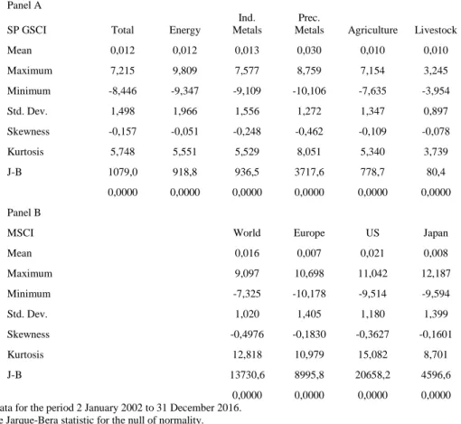
The main descriptive statistics on Stock and Commodity indices are presented in table 1. The analysis of these statistics allows conclude that, without exception the indexes presents a positive, although small, mean return.

The Jarque-Bera test has applied, in order to verify the adjustment of the normal distribution to the empirical distributions of series, whose statistical probabilities are presented in table 1. The results allow us to conclude that the series of logarithmic variations are statistically significant to 1%, clearly rejecting the hypothesis of their normality.

Table 1: Descriptive statistics

Panel A

SP GSCI Total Energy

Ind. Metals

Prec.

Metals Agriculture Livestock Mean 0,012 0,012 0,013 0,030 0,010 0,010 Maximum 7,215 9,809 7,577 8,759 7,154 3,245 Minimum -8,446 -9,347 -9,109 -10,106 -7,635 -3,954 Std. Dev. 1,498 1,966 1,556 1,272 1,347 0,897 Skewness -0,157 -0,051 -0,248 -0,462 -0,109 -0,078 Kurtosis 5,748 5,551 5,529 8,051 5,340 3,739 J-B 1079,0 918,8 936,5 3717,6 778,7 80,4 0,0000 0,0000 0,0000 0,0000 0,0000 0,0000 Panel B

MSCI World Europe US Japan

Mean 0,016 0,007 0,021 0,008 Maximum 9,097 10,698 11,042 12,187 Minimum -7,325 -10,178 -9,514 -9,594 Std. Dev. 1,020 1,405 1,180 1,399 Skewness -0,4976 -0,1830 -0,3627 -0,1601 Kurtosis 12,818 10,979 15,082 8,701 J-B 13730,6 8995,8 20658,2 4596,6 0,0000 0,0000 0,0000 0,0000

Notes: Daily data for the period 2 January 2002 to 31 December 2016. J-B denotes the Jarque-Bera statistic for the null of normality.

In order to estimate the VaR/CVaR we use a non-parametric, a parametric and a semi-parametric approach, at 99% and 95% confidence level and rolling windows of 90, 250 and 520 days.

Tables 2 to 5 present the main VaR/CVaR results for stocks and commodities.

Table 2A

Total Commodities, VaR/CVaR estimated by non-parametric, parametric and semi-parametric models

All period Non-parametric Parametric Semi-parametric

VaR99 CVaR99 VaR95 CVaR95 VaR99 CVaR99 VaR95 CVaR95 VaR99 CVaR99 VaR95 CVaR95

Panel A: 90 days rolling window forecasting

(5)

Max 8,253 8,446 6,428 7,305 9,025 10,236 6,590 8,083 8,292 9,466 6,407 7,539

Min 1,158 1,244 0,808 0,960 1,194 1,358 0,853 1,066 1,111 1,272 0,792 0,992

Std 1,418 1,550 1,012 1,175 1,326 1,506 0,966 1,187 1,375 1,684 0,954 1,204 Panel B: 250 days rolling window forecasting

Mean 3,612 4,126 2,353 3,118 3,273 3,752 2,310 2,900 3,712 4,581 2,332 3,193

Max 7,082 7,836 5,367 6,411 6,903 7,868 4,962 6,152 7,279 8,716 4,978 6,382

Min 1,533 1,702 0,984 1,262 1,440 1,646 1,025 1,280 1,431 1,644 1,006 1,272

Mean 3,856 4,590 2,420 3,306 3,331 3,820 2,348 2,951 3,995 5,092 2,371 3,391

Max 6,482 7,346 4,181 5,519 5,434 6,217 3,860 4,824 6,494 8,570 3,928 5,450

Min 2,080 2,444 1,132 1,649 1,668 1,907 1,189 1,483 1,998 2,478 1,145 1,713

Std 1,256 1,392 0,780 1,030 0,948 1,085 0,673 0,842 1,167 1,567 0,695 0,978

Table 2B

Total Commodities, VaR/CVaR estimated by non-parametric, parametric and semi-parametric models

Crisis

Period Non-parametric Parametric Semi-parametric VaR99 CVaR99 VaR95 CVaR95 VaR99 CVaR99 VaR95 CVaR95 VaR99 CVaR99 VaR95 CVaR95

Mean 4,304 4,602 2,809 3,545 3,826 4,388 2,698 3,390 4,199 5,005 2,774 3,655

Max 8,253 8,446 6,428 7,305 9,025 10,236 6,590 8,083 8,292 9,466 6,407 7,539

Min 1,908 2,036 1,231 1,674 2,031 2,329 1,416 1,793 2,051 2,373 1,369 1,798

Mean 4,390 5,012 2,899 3,856 3,906 4,480 2,753 3,460 4,511 5,533 2,845 3,882

Max 7,082 7,836 5,367 6,411 6,903 7,868 4,962 6,152 7,279 8,716 4,978 6,382

Min 2,427 2,778 1,695 2,325 2,521 2,909 1,742 2,220 2,590 2,995 1,754 2,271

Mean 4,761 5,575 3,006 4,091 4,003 4,590 2,823 3,547 4,823 6,091 2,899 4,105

Max 6,482 7,346 4,181 5,519 5,434 6,217 3,860 4,824 6,494 8,570 3,928 5,450

Min 2,950 3,245 1,809 2,592 2,847 3,275 1,984 2,513 2,923 3,329 2,017 2,576

Std 1,445 1,593 0,836 1,151 1,024 1,166 0,740 0,914 1,350 1,837 0,737 1,121

Table 2C

Total Commodities, VaR/CVaR estimated by non-parametric, parametric and semi-parametric models Pre-Crisis Non-parametric Parametric Semi-parametric

Mean 3,258 3,449 2,227 2,765 3,244 3,727 2,272 2,868 3,152 3,599 2,235 2,797

Max 4,710 4,757 2,933 4,058 4,158 4,757 2,954 3,692 4,577 5,747 3,103 3,982

Min 2,298 2,375 1,392 1,850 2,066 2,388 1,417 1,816 2,108 2,388 1,459 1,855

Mean 3,440 3,728 2,250 2,895 3,285 3,774 2,303 2,905 3,309 3,878 2,262 2,908

(6)

Min 2,829 2,983 1,908 2,531 2,751 3,155 1,938 2,437 2,891 3,200 1,982 2,541

Mean 3,481 4,021 2,350 2,999 3,313 3,807 2,320 2,929 3,414 4,069 2,276 2,982

Max 4,148 4,448 2,568 3,365 3,516 4,040 2,471 3,110 3,770 4,500 2,502 3,287

Min 2,913 3,265 2,177 2,659 3,103 3,566 2,171 2,743 3,051 3,550 2,106 2,698

Std 0,288 0,355 0,109 0,160 0,116 0,134 0,082 0,103 0,160 0,234 0,077 0,126

Table 2D

Total Commodities, VaR/CVaR estimated by non-parametric, parametric and semi-parametric models Pos-Crisis Non-parametric Parametric Semi-parametric

Mean 2,868 3,187 1,728 2,247 2,438 2,782 1,744 2,169 2,740 3,396 1,729 2,362

Max 5,589 6,586 2,627 3,730 4,346 4,939 3,153 3,884 5,422 7,765 3,172 4,428

Min 1,158 1,244 0,808 0,960 1,194 1,358 0,853 1,066 1,111 1,272 0,792 0,992

Mean 2,734 3,329 1,718 2,344 2,406 2,748 1,718 2,140 3,036 3,999 1,709 2,548

Max 4,484 5,369 2,597 3,481 3,870 4,409 2,785 3,450 4,827 7,554 2,729 3,775

Min 1,533 1,702 0,984 1,262 1,440 1,646 1,025 1,280 1,431 1,644 1,006 1,272

Mean 3,011 3,831 1,698 2,553 2,443 2,795 1,736 2,169 3,459 4,766 1,755 2,838

Max 3,964 4,779 2,112 3,270 3,022 3,443 2,177 2,695 4,243 5,912 2,248 3,471

Min 2,080 2,444 1,132 1,649 1,668 1,907 1,189 1,483 1,998 2,478 1,145 1,713

Std 0,657 0,859 0,308 0,500 0,429 0,491 0,303 0,380 0,726 1,061 0,342 0,578

Table 3A

MSCI World, VaR/CVaR estimated by non-parametric, parametric and semi-parametric models All sample Non-parametric Parametric Semi-parametric

Mean 2,342 2,513 1,553 1,953 2,058 2,361 1,450 1,823 2,310 2,815 1,477 1,995

Max 7,302 7,325 6,282 6,941 7,903 8,989 5,719 7,059 8,137 11,453 5,637 7,166

Min 0,820 0,868 0,486 0,709 0,814 0,948 0,543 0,709 0,841 0,885 0,548 0,743

Mean 2,616 2,896 1,590 2,152 2,115 2,426 1,489 1,873 2,638 3,411 1,518 2,223

Max 7,192 7,264 4,399 5,776 5,593 6,384 4,002 4,977 7,288 11,027 4,013 5,936

Min 1,017 1,116 0,678 0,850 1,064 1,230 0,728 0,934 0,968 1,051 0,722 0,872

Mean 2,859 3,495 1,621 2,359 2,232 2,560 1,572 1,977 3,060 4,167 1,588 2,522

Max 6,134 6,941 3,092 4,737 4,243 4,854 3,030 3,774 7,026 11,347 3,011 5,436

Min 1,053 1,163 0,745 0,950 1,129 1,303 0,779 0,994 1,079 1,219 0,769 0,958

(7)

Table 3B

MSCI World, VaR/CVaR estimated by non-parametric, parametric and semi-parametric models

Non-parametric Parametric Semi-parametric

Crisis

Panel A: Rolling window (90 days)

Mean 3,345 3,523 2,334 2,865 3,009 3,444 2,132 2,670 3,352 4,085 2,156 2,901

Max 7,302 7,325 6,282 6,941 7,903 8,989 5,719 7,059 8,137 11,453 5,637 7,166

Min 1,674 1,768 0,942 1,434 1,386 1,594 0,969 1,225 1,566 1,905 0,974 1,347

Mean 3,934 4,219 2,334 3,187 3,051 3,493 2,162 2,707 3,902 5,119 2,195 3,272

Max 7,192 7,264 4,399 5,776 5,593 6,384 4,002 4,977 7,288 11,027 4,013 5,936

Min 1,540 2,096 0,973 1,411 1,253 1,444 0,869 1,105 1,777 2,300 0,980 1,479

Mean 4,124 4,865 2,218 3,314 3,014 3,452 2,134 2,674 4,387 6,139 2,144 3,573

Max 6,134 6,941 3,092 4,737 4,243 4,854 3,030 3,774 7,026 11,347 3,011 5,436

Min 1,591 2,063 1,000 1,402 1,362 1,568 0,949 1,202 1,688 2,139 0,996 1,429

Std 1,715 1,874 0,688 1,198 0,982 1,118 0,708 0,876 1,812 2,848 0,674 1,399

Table 3C

MSCI World, VaR/CVaR estimated by non-parametric, parametric and semi-parametric models Pre-Crisis Non-parametric Parametric Semi-parametric

Mean 1,412 1,534 0,884 1,144 1,271 1,464 0,883 1,121 1,361 1,611 0,903 1,186

Max 2,116 2,515 1,491 1,730 1,981 2,263 1,413 1,761 2,014 2,898 1,392 1,744

Min 0,820 0,868 0,486 0,709 0,814 0,948 0,543 0,709 0,841 0,885 0,548 0,743

Mean 1,481 1,685 0,950 1,239 1,321 1,522 0,917 1,165 1,474 1,794 0,937 1,270

Max 2,178 2,396 1,302 1,746 1,838 2,122 1,269 1,618 2,105 2,642 1,284 1,796

Min 1,017 1,116 0,678 0,850 1,064 1,230 0,728 0,934 0,968 1,051 0,722 0,872

Mean 1,723 2,103 1,091 1,474 1,551 1,784 1,082 1,370 1,755 2,197 1,075 1,501

Max 2,928 3,372 1,812 2,373 2,541 2,912 1,795 2,252 2,883 3,780 1,711 2,430

Min 1,053 1,163 0,745 0,950 1,129 1,303 0,779 0,994 1,079 1,219 0,769 0,958

Std 0,574 0,604 0,340 0,434 0,452 0,517 0,323 0,402 0,527 0,719 0,287 0,440

Table 3D

MSCI World, VaR/CVaR estimated by non-parametric, parametric and semi-parametric models Pos Crisis Non-parametric Parametric Semi-parametric

(8)

Mean 1,921 2,130 1,168 1,529 1,563 1,795 1,097 1,383 1,852 2,306 1,134 1,582

Max 3,372 3,794 2,175 2,742 2,512 2,868 1,802 2,237 3,257 4,305 1,954 2,752

Min 1,071 1,154 0,663 0,880 0,897 1,034 0,621 0,791 1,059 1,224 0,657 0,929

Std 0,628 0,800 0,335 0,458 0,410 0,464 0,300 0,367 0,612 0,848 0,325 0,500

Panel B: 250 days rolling window forecasting

Mean 1,968 2,320 1,224 1,667 1,643 1,887 1,151 1,453 2,092 2,720 1,185 1,756

Max 4,395 4,708 2,290 3,353 3,221 3,684 2,292 2,862 4,074 5,256 2,395 3,443

Min 1,338 1,659 0,832 1,172 1,143 1,315 0,795 1,009 1,417 1,767 0,840 1,202

Std 0,679 0,718 0,333 0,474 0,476 0,543 0,340 0,423 0,599 0,823 0,333 0,496

Panel B: 520 days rolling window forecasting

Mean 2,284 3,033 1,343 1,952 1,855 2,130 1,301 1,641 2,571 3,471 1,348 2,122

Max 3,530 4,395 1,918 2,834 2,648 3,035 1,869 2,347 3,679 5,123 1,953 2,995

Min 1,527 1,783 0,949 1,301 1,291 1,488 0,896 1,139 1,507 1,870 0,929 1,290

Std 0,713 1,006 0,335 0,554 0,516 0,589 0,368 0,459 0,738 1,023 0,374 0,605

Table 4

MSCI World, MSCI Europe, MSCI US and MSCI Japan, VaR/CVaR estimated by non-parametric, parametric and semi-parametric models

all sample Non-parametric Parametric Semi-parametric

Panel A: 520 days rolling window forecasting - MSCI WORLD

Mean 2,859 3,495 1,621 2,359 2,232 2,560 1,572 1,977 3,060 4,167 1,588 2,522

Max 6,134 6,941 3,092 4,737 4,243 4,854 3,030 3,774 7,026 11,347 3,011 5,436

Min 1,053 1,163 0,745 0,950 1,129 1,303 0,779 0,994 1,079 1,219 0,769 0,958

Std 1,600 1,795 0,713 1,173 0,977 1,114 0,702 0,871 1,689 2,569 0,685 1,326 Panel B: 520 days rolling window forecasting - MSCI EUROPE

Mean 3,779 4,578 2,189 3,168 3,080 3,532 2,173 2,729 4,048 5,484 2,141 3,352

Max 6,978 8,300 3,982 5,753 5,560 6,358 3,956 4,939 8,616 13,521 3,708 6,646

Min 1,566 1,720 1,053 1,346 1,537 1,774 1,062 1,353 1,507 1,732 1,050 1,330

Std 1,684 1,935 0,895 1,335 1,242 1,416 0,892 1,106 1,876 2,859 0,801 1,483 Panel C: 520 days rolling window forecasting - MSCI US

Mean 3,219 4,035 1,851 2,696 2,586 2,966 1,822 2,290 3,576 4,929 1,812 2,934

Max 6,575 8,586 3,508 5,505 5,178 5,918 3,691 4,602 8,581 14,226 3,552 6,600

Min 1,486 1,573 0,989 1,261 1,403 1,613 0,978 1,239 1,459 1,707 0,959 1,281

Std 1,658 2,297 0,791 1,359 1,191 1,360 0,853 1,060 2,107 3,267 0,801 1,637 Panel D: 520 days rolling window forecasting - MSCI JAPAN

Mean 3,683 4,978 2,194 3,187 3,195 3,662 2,255 2,831 4,469 6,157 2,263 3,665

Max 6,245 7,637 3,571 5,190 5,144 5,881 3,662 4,571 7,621 11,855 3,524 5,927

Min 2,417 2,848 1,547 2,084 2,250 2,582 1,584 1,993 2,389 2,815 1,519 2,092

Std 1,073 1,212 0,549 0,839 0,793 0,903 0,572 0,707 1,328 2,225 0,489 1,004

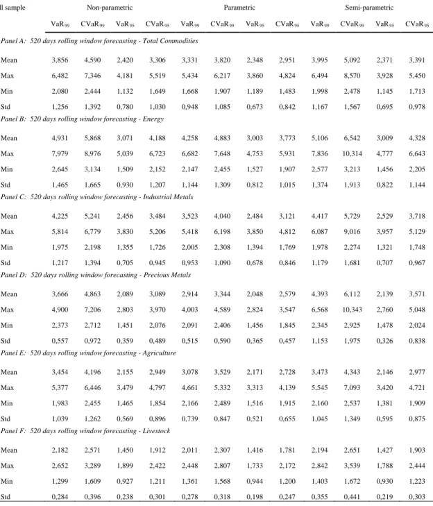
Table 5

SP Total Commodities, Energy, Industrial Metals, Precious Metals, Agriculture and Livestock, VaR/CVaR estimated by non-parametric, parametric and semi-parametric models

(9)

all sample Non-parametric Parametric Semi-parametric

Panel A: 520 days rolling window forecasting - Total Commodities

Mean 3,856 4,590 2,420 3,306 3,331 3,820 2,348 2,951 3,995 5,092 2,371 3,391

Max 6,482 7,346 4,181 5,519 5,434 6,217 3,860 4,824 6,494 8,570 3,928 5,450

Min 2,080 2,444 1,132 1,649 1,668 1,907 1,189 1,483 1,998 2,478 1,145 1,713

Std 1,256 1,392 0,780 1,030 0,948 1,085 0,673 0,842 1,167 1,567 0,695 0,978 Panel B: 520 days rolling window forecasting - Energy

Mean 4,931 5,868 3,071 4,188 4,258 4,883 3,003 3,773 5,106 6,542 3,009 4,328

Max 7,979 8,976 5,039 6,723 6,682 7,648 4,753 5,931 7,836 10,314 4,777 6,643

Min 2,645 3,134 1,509 2,152 2,147 2,455 1,527 1,907 2,577 3,213 1,456 2,205

Std 1,465 1,665 0,930 1,207 1,144 1,309 0,812 1,015 1,374 1,913 0,822 1,144 Panel C: 520 days rolling window forecasting - Industrial Metals

Mean 4,225 5,241 2,456 3,484 3,523 4,040 2,484 3,121 4,417 5,729 2,529 3,718

Max 5,814 6,779 3,830 5,206 5,418 6,198 3,850 4,812 6,087 9,016 3,957 5,129

Min 1,975 2,198 1,355 1,726 2,005 2,308 1,394 1,769 1,978 2,274 1,321 1,748

Std 1,217 1,394 0,705 0,945 0,953 1,090 0,678 0,846 1,179 1,681 0,707 0,967 Panel D: 520 days rolling window forecasting - Precious Metals

Mean 3,666 4,863 2,089 3,089 2,914 3,344 2,048 2,579 4,393 6,112 2,139 3,571

Max 4,900 7,206 2,803 3,970 4,003 4,589 2,824 3,547 6,568 10,343 2,760 5,048

Min 2,373 2,712 1,451 2,076 2,091 2,406 1,456 1,845 2,345 2,925 1,478 2,024

Std 0,557 0,972 0,359 0,489 0,515 0,590 0,365 0,457 1,153 1,975 0,326 0,838 Panel E: 520 days rolling window forecasting - Agriculture

Mean 3,454 4,196 2,155 2,949 3,078 3,529 2,171 2,728 3,473 4,343 2,146 2,977

Max 5,377 6,446 3,479 4,797 4,661 5,332 3,313 4,139 5,545 7,093 3,420 4,721

Min 1,983 2,455 1,465 1,854 2,166 2,489 1,516 1,915 2,160 2,537 1,381 1,909

Std 1,039 1,262 0,569 0,896 0,739 0,847 0,521 0,655 1,045 1,349 0,595 0,875 Panel F: 520 days rolling window forecasting - Livestock

Mean 2,182 2,571 1,450 1,912 2,011 2,307 1,416 1,781 2,194 2,651 1,427 1,903

Max 2,652 3,289 1,899 2,422 2,448 2,807 1,733 2,172 2,842 3,539 1,788 2,444

Min 1,299 1,609 0,927 1,211 1,361 1,568 0,944 1,200 1,403 1,672 0,930 1,223

Std 0,284 0,396 0,238 0,301 0,278 0,318 0,198 0,247 0,355 0,441 0,219 0,303

Nonparametric and semi-parametric methods have performed well during all period. However, the behaviour of the models is not constant over time. During the crisis period all CVaR models included, using nonparametric and semi-parametric methods was accepted at both confidence levels, while almost included VaR models were rejected.

Figures 1a to 1d CVaR show the daily CVaR based on a rolling window of 520 days and a confidence level of 95%, for the pairs formed by each stock market index MSCI World, Europe, US and Japan, and each commodity index.

(10)

Fig. 1b. CVaR 95%. MSCI Europe vs Commodities -.10 -.08 -.06 -.04 -.02 .00 04 05 06 07 08 09 10 11 12 13 14 15 16 Total Commodities MSCI World

CVaR 95% -.10 -.08 -.06 -.04 -.02 .00 04 05 06 07 08 09 10 11 12 13 14 15 16 Energy MSCI World

CVaR 95% -.10 -.08 -.06 -.04 -.02 .00 04 05 06 07 08 09 10 11 12 13 14 15 16 Industrial Metals MSCI World

CVaR 95% -.10 -.08 -.06 -.04 -.02 .00 04 05 06 07 08 09 10 11 12 13 14 15 16 Precious Metals MSCI World

CVaR 95% -.10 -.08 -.06 -.04 -.02 .00 04 05 06 07 08 09 10 11 12 13 14 15 16 Agriculture MSCI World

CVaR 95% -.10 -.08 -.06 -.04 -.02 .00 04 05 06 07 08 09 10 11 12 13 14 15 16 Livestock MSCI World

(11)

Fig. 1c. CVaR 95% MSCI US vs Commodities -.14 -.12 -.10 -.08 -.06 -.04 -.02 .00 04 05 06 07 08 09 10 11 12 13 14 15 16 Total Commodities MSCI Europe

CVaR 95% -.14 -.12 -.10 -.08 -.06 -.04 -.02 .00 04 05 06 07 08 09 10 11 12 13 14 15 16 Energy MSCI Europe

CVaR 95% -.14 -.12 -.10 -.08 -.06 -.04 -.02 .00 04 05 06 07 08 09 10 11 12 13 14 15 16 Industrial Metals MSCI Europe

CVaR 95% -.14 -.12 -.10 -.08 -.06 -.04 -.02 .00 04 05 06 07 08 09 10 11 12 13 14 15 16 Precious Metals MSCI Europe

CVaR 95% -.14 -.12 -.10 -.08 -.06 -.04 -.02 .00 04 05 06 07 08 09 10 11 12 13 14 15 16 Agriculture MSCI Europe

CVaR 95% -.14 -.12 -.10 -.08 -.06 -.04 -.02 .00 04 05 06 07 08 09 10 11 12 13 14 15 16 Livestock MSCI Europe

(12)

Fig. 1d. CvaR 95%. MSCI Japan vs Commodities -.12 -.10 -.08 -.06 -.04 -.02 .00 04 05 06 07 08 09 10 11 12 13 14 15 16 Total Commodities MSCI US

CVaR 95% -.12 -.10 -.08 -.06 -.04 -.02 .00 04 05 06 07 08 09 10 11 12 13 14 15 16 Energy MSCI US CVaR 95% -.12 -.10 -.08 -.06 -.04 -.02 .00 04 05 06 07 08 09 10 11 12 13 14 15 16 Industrial Metals MSCI US

CVaR 95% -.12 -.10 -.08 -.06 -.04 -.02 .00 04 05 06 07 08 09 10 11 12 13 14 15 16 Precious Metals MSCI US

CVaR 95% -.12 -.10 -.08 -.06 -.04 -.02 .00 04 05 06 07 08 09 10 11 12 13 14 15 16 Agriculture MSCI US CVaR 95% -.12 -.10 -.08 -.06 -.04 -.02 .00 04 05 06 07 08 09 10 11 12 13 14 15 16 Livestock MSCI US CVaR 95%

(13)

The analysis of figures allows us to observe the significant difference of magnitude of tail metrics during the crisis period and calm periods.

The CVaR of MSCI World and Total Commodities presented at the top left in Figure 1a shows that tail risk of commodity market is much higher than stock market prior to the crisis period. The crisis period changed the pattern, as the tail risk of stock markets increase significantly, to the same levels of commodity indices. Similar pattern can also be observed for energy, industrial metals, precious metals and agricultural indices.

Not surprisingly, the US case shows as well as the global case that the post-crises display almost the pattern than pre-crises, while the European stock market continuous to present relatively high tail risk values in the post-crises period.

To infer the relations established between the performances of these tail risk measures we carry out the analysis of the dynamic conditional correlations, to stablish a set of co-movements between the two variables.

With the aim of analyse the time-varying correlations of stock markets returns and commodity indices we adopt the DCC model.

Fig. 2. Dynamic Conditional Correlations. -.12 -.10 -.08 -.06 -.04 -.02 .00 04 05 06 07 08 09 10 11 12 13 14 15 16 Total Commodities MSCI Japan

CVaR 95% -.12 -.10 -.08 -.06 -.04 -.02 .00 04 05 06 07 08 09 10 11 12 13 14 15 16 Energy MSCI Japan

CVaR 95% -.12 -.10 -.08 -.06 -.04 -.02 .00 04 05 06 07 08 09 10 11 12 13 14 15 16 Industrial Metals MSCI Japan

CVaR 95% -.12 -.10 -.08 -.06 -.04 -.02 .00 04 05 06 07 08 09 10 11 12 13 14 15 16 Precious Metals MSCI Japan

CVaR 95% -.12 -.10 -.08 -.06 -.04 -.02 .00 04 05 06 07 08 09 10 11 12 13 14 15 16 Agriculture MSCI Japan

CVaR 95% -.12 -.10 -.08 -.06 -.04 -.02 .00 04 05 06 07 08 09 10 11 12 13 14 15 16 Livestock MSCI Japan

(14)

In general, the contemporary conditional correlations between stock markets, measured by the MSCI World and commodities were positive for returns, with the exception of Agriculture and Livestock with a near zero correlation. The global financial crises and the sovereign debt crises clearly increased correlations between MSCI World index and commodities at global level, for energy, industrial metals and agriculture, although livestock remain unaltered, we can see a correlation decrease in precious metals.

At tail level less intense contemporaneous correlations is presented with frequent and strong oscillations suggesting a temporal mismatch. During crisis periods, the tail risk between Market return and commodity indices present higher contemporaneous correlations for all pairwise analysed. We can clearly notice that during the crisis period, especially during the global financial crisis, the highest values of these correlations occurred and settled

We can clearly see that during the crisis period, especially during the global financial crisis, when the highest values of these correlations were found, the correlations at the tails level were clearly higher than the correlations at the mean level.

6. CONCLUSION

This paper analyses the links between commodity and stock markets, considering the total and the tail risk. -1.00 -0.75 -0.50 -0.25 0.00 0.25 0.50 0.75 1.00 04 05 06 07 08 09 10 11 12 13 14 15 16 MSCI World and Total Commodities - CVaR

MSCI World and Total Commodities - Returns

-1.00 -0.75 -0.50 -0.25 0.00 0.25 0.50 0.75 1.00 04 05 06 07 08 09 10 11 12 13 14 15 16 MSCI World and Energy - CVaR

MSCI World and Energy - Returns

-1.00 -0.75 -0.50 -0.25 0.00 0.25 0.50 0.75 1.00 04 05 06 07 08 09 10 11 12 13 14 15 16 MSCI World and Industrial Metals - CVaR

MSCI World and Industrial Metals - Returns

-1.00 -0.75 -0.50 -0.25 0.00 0.25 0.50 0.75 1.00 04 05 06 07 08 09 10 11 12 13 14 15 16 MSCI World and Precious Metals - CVaR

MSCI World and Precious Metals - Returns

-1.00 -0.75 -0.50 -0.25 0.00 0.25 0.50 0.75 1.00 04 05 06 07 08 09 10 11 12 13 14 15 16 MSCI World and Agriculture - CVaR

MSCI World and Agriculture - Returns

-1.00 -0.75 -0.50 -0.25 0.00 0.25 0.50 0.75 1.00 04 05 06 07 08 09 10 11 12 13 14 15 16 MSCI World and Livestock - CVaR

(15)

To this end, we examining two tail risk measures - VaR and CVaR, with several approaches each commodity and stock market index over a period of fourteen years.

We study the consistence of measures over time, namely considering the periods of pre-crises, global financial and sovereign debt crisis and post-crisis. Using the dynamic conditional correlation (DCC) GARCH methodology to establish whether the correlations between commodity and stock market evolve over time and depend on the economy phase situation.

Our main findings can be summarized as follows.

First, in order to measure the tail risk, nonparametric and semi-parametric methods have performed well during all period. However, this behaviour of the considered methods is not constant over time.

Second, the tail risk of commodity markets is higher than stock market over the period, for energy, industrial metals, precious metals and agricultural indices as well as total commodities, but over the crisis period analysed the tail risk of stock market indices sharply increases to the same levels of commodities tail risk.

Third, the correlations between commodity and stock returns evolve through time. Considering the total returns, we can observe an increase of correlation over high volatility periods, particularly between 2007– 2012.

At tail risk level, for all analysed pairs, commodity and stock returns, present a very high contemporaneous correlations during the crisis period.

(16)

REFERENCES

Bauwens, L., S. Laurent and J.V.K. Rombouts (2006). “Multivariate GARCH Models: A Survey,” Journal of Applied Econometrics, vol. 21, pp. 79-109.

Choi, K. and S. Hammoudeh (2010), “Volatility behavior of oil, industrial commodity and stock markets in a regime-switching environment”, Energy Policy, 38 (8), pp. 4388-4399.

Creti, A., Joëts, M. and V. Mignon, (2013), “On the links between stock and commodity markets' volatility”, Energy Economics, vol. 37, pp. 16-28.

Engle, R. (2002): “Dynamic Conditional Correlation: A Simple Class of Multivariate GARCH Models”. Journal of Business and

Economic Statistics, vol. 20, pp 339-350.

Maillard, D. (2018), “A user’s guide to the Cornish Fisher expansion”, Working Paper, p. 18, 2018

Malik, F. and B.T. Ewing (2009), “Volatility transmission between oil prices and equity sector returns”, International Review of

Financial Analysis, vol. 18, pp. 95-100.

Park,J. and R.A. Ratti (2008), “Oil price shocks and stock markets in the U.S. and 13 European countries”, Energy Economics, vol. 30, pp. 2587-2608

Powell, R.J. Vo,D.C. Pham,T.N. and Abhay K. Singh, (2017), The long and short of commodity tails and their relationship to Asian equity markets, Journal of Asian Economics, vol. 52, pp. 32-44,

Rockafellar, R.T. and S. Uryasev. (2000), “Optimization of conditional value-at-risk”, Journal of Risk, vol. 2, pp. 21-41.

Silvennoinen, A and T. Terasvirta (2008), “Multivariate GARCH Models,” Handbook of Financial Time Series. In T.G. Andersen, R.A. Davis, J.P. Kreiss and T. Mikosch, eds., New York: Springer.

Tse, Y.K. and Tsui, A.K.C. (2002), “A multivariate generalized autoregressive conditional heteroscedasticity model with time-varying correlations”, Journal of Business and Economic Statistics, vol. 20 (3), pp. 351-362