Unilever Group : equity valuation

(1)

Equity Valuation

Unilever Group

Candidate:

Susana Pires

152112095

susana.pires@yahoo.com

Supervisor:

Dr. José Carlos Tudela Martins

Dissertation submitted in partial fulfillment of requirements for the degree of MSc in Business Administration, at the University Católica Portuguesa.

(2)

Page | ii 20.00 22.00 24.00 26.00 28.00 30.00 32.00 34.00 01 /2 01 2 04 /2 01 2 07 /2 01 2 10 /2 01 2 01 /2 01 3 04 /2 01 3 07 /2 01 3 10 /2 01 3 01 /2 01 4 04 /2 01 4 07 /2 01 4 Unilever's Historical Prices Dissertation's Target Price J. P. Morgan's Target Price

“UNILEVER: WATCH OUT! TIME TO INVEST”

Unilever is a global warrior fighting its competitors and adverse market conditions mainly in result of the economic crisis. Even in a mature and too competitive market, Unilever has found its way to make it noticeable to consumers and have a very healthy capital structure – being its credit rated at A+ by Standard & Poor’s.

Its wide brand portfolio is segmented into 4 businesses – Personal Care, Foods, Refreshment and Home Care products – being somewhat able to diversify the risk within the market. This year in particular, 2014, has been quite challenging since high expectations and goals were made but the market is the one that dictates its future. Therefore, Unilever has already been rearranging its goals for the year and changing its operational strategy (for instance, increasing its mix of prices according to the inflation behavior). Furthermore, the aligned main priorities for 2014 are to reach a volume growth ahead of its markets, a steady and sustainable improvement in core operating margin, and strong cash flows.

Being all that said, even with the current struggles, an opportunity must be given to Unilever since it is expected to improve ahead. This report is based on thorough research of public information in order to make reliable assumptions regarding Unilever operations. Moreover, a DCF-WACC based methodology was performed estimating a target price of €36.39. Since the market is yielding to a price of €31.86 at 24th_{July of 2014, a buy recommendation will be}

issued.

2014

RECOMMENDATION

BUY

TARGET PRICE

€36.39

CURRENT COMPANY INFO

Price @ 24/07/2014: €31.86 Shares O/S (Million): 2,840

VALUATION TARGET

EV (€M): 108,799

Mkt Value of Equity (€M): 103,356 Target Price (€): €36.39 Shares O/S (Million): 2,840

Date of Price: 24/07/2014

J.P. MORGAN VALUATION TARGET

Target Price: €27.00 52-week range: €32.72 – 26.97

Shares O/S (Million): 2,829 Date of Price: 24/07/2014

CREDIT RATING

(3)

Page | iii

ABSTRACT

The following dissertation has the purpose to value the Unilever Group, but more specifically Unilever N.V. being publicly traded in the Amsterdam Exchange Index. Unilever is seen as a global player and one of most successful and competitive fast-moving consumer goods companies. In order to valuate Unilever’s equity, a Discounted Cash Flow (DCF) approach is first carried out, since it is believed to be the most reliable methodology. The value estimated was €36.39, advising one to buy its shares when comparing to the actual price of € 31.86.

Further on, a relative valuation (selecting a specific peer group and applying multiples) is suggested, as a complementary analysis to the DCF, leading to a target price of €34.15 using a forward enterprise-value multiple for 2014. Meaning, once again, a buy recommendation is issued, since the market currently yields a lower value.

As a final assessment and basing the target price on the present value of future dividends, a Dividend Discount Model (DDM) is performed. This model indicates Unilever’s is priced at €18.65, leading to an overvalued market price and, consequently, a selling opportunity.

Lastly, a comparison is made between these results and the target price reached by a JP Morgan’s analyst, being the last one priced at €27.00 using a DCF-WACC methodology (representing a selling opportunity). All details are further addressed in this Thesis.

(4)

Page | iv

ACKNOWLEDGMENTS

Since this experience has been quite a rollercoaster ride, all the support and motivation received was determinant to accomplish yet another great challenge and get to succeed at the end.

Firstly, I would like to thank my advisor, Professor José Tudela Martins, for all his guidance and availability leading me into the right path.

All my gratitude goes to Horácio Cal, Chief Sales Officer of Olá and Lipton at Unilever Jerónimo Martins, who kindly shared relevant internal information in order to conceptualize my assumptions.

And finally, a special thanks to my parents for the unconditional support and to all my friends who accompanied me in this journey by giving constructive suggestions and supporting me all the way. I believe after this era, I will leave as a wiser and responsible professional, but also a better and stronger individual.

(5)

Page | 5

1 LITERATURE REVIEW

1.1 INTRODUCTION

In order for a company to assess if its future events and strategic decisions might bring success or failure to its activity, a valuation tool is usually used. Luehrman (1997) refers that those decisions are related to resource allocation and it creates a direct impact on the company’s value.

“(…) how a company estimates value is a critical determinant of how it allocates resources” and this allocation is “a key driver of a company’s overall performance”

– LUEHRMAN, 1997

Luehrman (1997) also refers this resource allocation brings three issues into the valuation – operations, opportunities and ownership claims – which must be valued correctly, according to three fundamental factors – cash, timing and risk.

Furthermore, those three issues can be valuated through choosing a tool from a diverse portfolio of valuation approaches. However, a somewhat deep analysis into the structural features and the kind of major decisions managers face must be done in order to find a match in terms of the tool to choose from.

Any analysis, however, is only as accurate as the forecasts it relies on (Goedhart et. al, 2005). Errors while estimating the key ingredients of corporate value ingredients such as a company’s return on invested capital (ROIC), its growth rate, and its weighted average cost of capital (WACC) can lead to mistakes in valuation and, ultimately, to strategic errors.

Young et al. (1999) claims that there are so many valuation approaches that managers might tend to use every single one that fits just because. In fact it is referred that higher number of approaches used leads to a weaker message in terms of final conclusions for the valuation. The paper offers a step-by-step guide in order to cut through this complexity, by stating that every valuation approach are mathematically equal since they represent only a different way of expressing the same underlying model. Therefore, four main practical implications are defended to be relevant for this logical thinking – consistency of the data and of the assumptions; comparison between models; uniqueness of the one single fair value estimation; and, consistency without uniformity, in which all analysts should be free to decide about the valuation approach to use (Young et al., 1999).

In this chapter, several valuation frameworks will be mentioned and explained in order to find adequate ones for this Thesis – including the discounted cash flow based ones, the multiples approach and options, between others – and relevant variables for this purpose will also be clarified. At the end of all sections, a final comment will be made related to the ones which will be used afterwards during the valuation.

(9)

Page | 9

1.2 VALUATION MODELS

1.2.1 THE DISCOUNTED CASH FLOWS METHOD

The discounted cash flow (DCF) method is based upon expected future cash flows discounted at a risk rate according to the type of cash flow associated.

Value of Assets E(CF1) (1+r) + E(CF₂) (1+r)2+ E(CF₃) (1+r)3+…+ E(CF_n) (1+r)n (1) Where:

= Expected Cash Flow in period t

r = discount rate according to the associated risk of each estimated cash flow n = life period of asset

Valuations based on this approach take into account free cash flows, having two different perspectives – Free Cash Flow to the Firm (FCFF) and Free Cash Flow to the Equity (FCFE). The first one is characterized by the sum of the cash flows to all claim holders in the firm, including stockholders, bondholders and preferred stockholders (Damodaran, 2002). The relationship between these two variables can be explained as follows:

( ) ( ) (2) ) Where: = Interest rate Being, (3)

Both approaches would represent at the end the same value, however the methodology behind them is different since the first one (FCFF) is discounted at a constant rate, called weighted average cost of capital (WACC), whereas the latter is at cost of equity.

ACC ( )

(4)

Where:

= Market Value of Debt V= Market Value of the Firm t = tax rate

E = Market Value of Equity = cost of debt

(10)

Page | 10 WACC is a tax-adjusted discount rate since it reflects the interest tax shields’ value while using an operation’s debt capacity. On one hand, using a constant rate such as this one for all expected cash flows of a firm can make calculations quite simple and keep them to a minimum (Luehrman, 1997). On the other hand, this simplicity is not considered suitable for any situation, but only for the simplest and most static of capital structures.

According to Damodaran (2002), this model is proper for companies or assets with currently positive cash flows and for those that can reliably estimate values for future periods. In addition, it can only be used to obtain discount rates when a proxy for risk is available.

However, as every other model, it is not perceived as a perfect one. And DCF has its own limitations to when it comes to: distressed firms with negative earnings and cash flows and/or which expect to lose money for some time in the future; cyclical firms with earnings and cash flows following the economy – rising during economic booms and failing during recessions – which lead to a “smoothed out” of expected future CFs; firms with unutilized assets which means assets that do not produce any cash flows to the firm having then no impact when discounting expected future cash flows; firms with patents or product options (which don’t produce any current CFs and do not expect future ones but they are perceived as valuable) that will lead to a understate of firm value; firms in the process of restructuring (in which may happen some asset sale or acquisition, for example) which may difficult the estimation of those future CFs and also will affect the riskiness of the firm; firms involved in acquisitions due to the difficulty in estimating the value of those synergies; and finally, for private firms since internal and relevant information is not public and therefore the measurement of the risk (used when estimating discount rates) is quite difficult.

1.2.2 THE ADJUSTED PRESENT VALUE METHOD

Since ACC is seen as a limited “opportunity cost” for all cash flows, few corrections might be done in order to achieve a more realistic model. In this case, the adjusted present value (APV) method is the solution. Using this one, WACC can be adjusted beyond tax shields. In fact, APV will now take into account further criterion, such as issue costs, subsidies, hedges, exotic debt securities, and dynamic capital structures.

In addition, these adjustments must be taken into consideration in accordance to the kind of project and period which are being used in each case. Also, as referred previously, a DCF valuation methodology may incur in more mistakes and errors when valuating companies with a very complex capital structures, tax position, or fund-raising strategy – Luehrman, 1997.

This methodology starts by estimating the value of the firm with no leverage (discounting the expected FCFF at the unlevered cost of equity and using an unlevered beta of the firm). Afterwards, the leverage variable will be taken into consideration by estimating the present value of the interest tax savings. This value is described as a borrowed amount of money and its further valuation based

(11)

Page | 11 upon the probability that the firm will go bankrupt and the expected cost of bankruptcy. This probability might be estimated through bond rating or using a statistical approach (for instance a probit(1)_{to estimate the probability of default, taking in to consideration the firm’s observable}

characteristics, at each level of debt).

(5)

All in all, APV model takes a project and breaks it into several managerial parts, values each one according to its properties and then adds them back up – relying on the principle of value additivity – Luehrman, 1997.

Damodaran (2002) considers APV as a more flexible approach. When analyzing bankruptcy costs, this model takes into consideration also the indirect ones which can yield to a more conservative estimation of the value. In addition, the APV model shows tax benefit as a dollar debt value (based on existing debt), whereas DCF estimates tax benefit from debt ratio leading consequently to future borrows of great amount.

To sum up, APV separates the effects of debt into different components and allows using different discount rates for each component, becoming more realistic. And also, APV takes into account that the debt ratio may not stay unchanged throughout time. Instead, it becomes more flexible by keeping the dollar value of debt fixed and calculating its benefits and costs.

Nevertheless, there are also a few limitations to this model, such as the difficulty of estimating probabilities of default and the cost of bankruptcy, and it is not that easy to use when firms are analyzing debt proportions. In the latter case, the DCF method would be more suitable.

1.2.3 RELATIVE VALUATION

Goedhart et al. (2005) stress that using a multiples analysis, can bring many benefits for a company, starting by being a tool to forecast its cash flows and to compare its performance and value creation (by being well strategically positioned, for instance) to other industry players. After all, this kind of analysis can give some insights into the strategy and key factors of a company or even an industry. Yet, multiples are often misapplied and misunderstood.

Damodaran (2002) refers the main advantage of using a relative valuation which is the simplicity and easiness to work with. Furthermore, it becomes quite useful whenever a large number of comparable firms are being traded on financial markets and the market is pricing them, on average, correctly.

1_{Probit is a regression model in which the dependent variable is only able to acknowledge two values, being}

(12)

Page | 12 On the other hand, has a limited use whenever the comparables are not that obvious mainly due to the subjective meaning of “comparable” since perspectives and opinions may differ between analysts. Consequently, it is easy to misuse and manipulate this valuation. In addition, following what was referred previously on this subject, the valuation depends mainly on how the market is pricing those comparable firms, which means this valuation might be built in errors (overvaluation or undervaluation) – Damodaran, 2002.

Furthermore, Goedhart et al. (2005) include three major problems while using multiples for a company’s valuation. Firstly, “investors have different expectations about each company’s ability to create value going forward”. An accurate comparable has to be one with similar expectations when it comes to growth and ROIC variables. Secondly, “different multiples can suggest conflicting conclusions when interpreting and comparing results between different multiples from comparables”. Finally, “different multiples are meaningful in different contexts”. Many corporate managers believe that growth rates and multiples do not follow that same pattern. For instance, one must take into account growth and returns on capital when making conclusions through this analysis. P/E multiple is increased due to a positive growth, but only when there are healthy returns on invested capital. And, this aspect can vary across companies. Therefore, not taking those two variables into consideration, can lead to a situation where a company has achieved its growth objectives but forfeit the benefits of a higher P/E.

Goedhart et al. (2005) explain as well the four basic principles which can help companies to apply multiples properly. Firstly, one should choose peers with similar expectations for ROIC and growth. In order to choose suitable ones, one needs to list a company’s competitors and examine each one regarding operating and financial aspects – for instance, what kind of products they are selling, how they generate profits and revenues, and how is their growth – in order to end up with a smaller number of reliable and comparable peers. Secondly, one should not use multiples based on historical profits, but based on future events. Moreover, P/E multiples may incur in error due to varying according to a company’s capital structure and to being based on earnings which include many non-operating items. Therefore, using enterprise-value multiples is preferable. For example, changes in capital structure do not have a great impact on the enterprise-value-to-EBITDA multiple – except when such change lowers the cost of capital, which will lead to a higher value for this multiple. Also, the latter multiple needs to suffer some adjustments related to non-operating items (such as excess cash and operating leases).

Nevertheless, depending on the type of situation, other multiples can be used. For instance, price-to-sales multiples have their own limitations since it assumes that comparable companies need to have similar perspectives of growth, ROIC and operating margins.

PEG ratios (comparing a company’s P/E ratio with its underlying growth rate in earnings per share) are more flexible since they allow the expected level of growth to vary across companies. Therefore, it becomes easier to valuate companies in different stages of the life cycle – meaning different

(13)

Page | 13 growth rates. However, a standard time frame in order to measure expected growth of a company is hard to achieve with this kind of ratio and they assume a linear relation between multiples and growth – which means a company can have a null multiple or even being undervalued when there is no growth or a low growth rate, respectively.

Furthermore, in case of evaluating a company with small sales and negative profits, nonfinancial multiples may be more suitable, even acknowledging the uncertainty related to the potential market size and to these companies’ profitability or the investments they require. After all, nonfinancial multiples compare enterprise value to a non-operating statistic, however they should be used only when they achieve more realistic values than financial ones do. Also, like all multiples, nonfinancial ones are only relative tools and they merely measure one company’s valuation compared with another’s.

In what concerns multiple estimation, Liu et al. (2002) believes a harmonic average, using all companies within the peer group, needs to be taken into consideration since it yields more reasonable results regarding the performance of the company in analysis.

1.2.4 OPTION PRICING THEORY AND MODELS

When it comes to valuing opportunities within a company, Luehrman (1997) believes this approach to be the best. Being so, a common approach is to value those opportunities only when they reach maturity – the point where an investment decision can no longer be deferred. Not doing so, usually yields to undervaluing the future and hence, to underinvest. In addition, not having a formal valuation procedure may rise to personal and informal statements affecting the evaluation.

In financial terms, an opportunity is comparable to an option. This analogy is due to having the right – but not the obligation – to exercise the option to purchase or sale of an item at a specified price until a determined future date. And corporate opportunities are seen as the same when it comes to investment decisions around those opportunities – the action of investing on some opportunity is analogous to exercise an option (Luehrman, 1997). So, one is able to provide a value to an option which depends on the value of the underlying asset – the stock. Yet, in terms of ownership it is not so linear, since the ownership of a stock has not the same meaning or value of owning the option.

Several variables are taken into consideration, firstly with the cash from the business and the cash needed in case one decides to enter it. In addition, the timing of its flows and the chance of deferring an investment decision and its duration are both of great importance. And, finally, the risk variable must not be forgotten. When investing in a business, one needs to take in to account whether that business is risky or not, and whether its circumstances may or not change before the decision deadline.

(14)

Page | 14 One needs to be able to acknowledge the analogous characteristics of a project and an option. First, an option’s exercise price corresponds to the expected investment in those opportunities. Consequently, exercising a call option and owning afterwards the stock is like the operating assets a company would own after the investment. Following the same logic, the length of time waited for the company to make a decision is comparable to the expiration time of a call option.

As every other project, uncertainty plays a major role in decision-making situations. In fact, the future value of an asset (operating ones or call options, for instance) captures uncertainty which is determined by the behavior of those assets’ returns.

Concerning options valuation, the Black-Scholes model is the most used one. The major limitation of this approach is that it is “designed to value options that can be exercised only at maturity and on underlying assets that do not pay dividends” – Damodaran, 2002.

Therefore, a possibility to overcome this issue is to include the dividends variable whether it is a short- or long-term option. Unquestionably, paying dividends will reduce the stock price leading to an increase in value for put options and the other way around for call options. Being so, in case of dealing with short-term options, the methodology is to estimate the present value of expected dividends that will be paid by the underlying asset and deduct this value to the current stock price (S’ – modified stock price). Otherwise, if a long-term option is being analyzed, one ought to control whether the dividend yield (y – dividends under current value of the asset) on the underlying asset is expected to remain constant during the option’s life.

In case of having long-term scoped opportunities in a business environment suffering with high volatility, a DCF methodology would not be considered wise to use, since no reliable conclusions can be estimated. And in these cases, one does not need to have a very refined and complex option-pricing analysis in order to achieve some meaningful conclusions.

Furthermore, while choosing different valuation methodologies, Luehrman (1997) advises to use option pricing as a complementary analysis, and not as a replacing one. A practical way to use this kind of analysis is to run it afterwards a DCF analysis, since its outputs will become the inputs for option-pricing.

Finally, in terms of costs, this one is costlier and quite accessible. However it is less intuitive leading one to learn more about the tool and further procedures.

1.2.5 DIVIDEND DISCOUNT MODEL

Joint ventures, partnerships, or strategic alliances, or investments using project financing give the opportunity to companies to diversify their investments and share risk with other parties. Furthermore, they are sharing ownership. Thus, the venture value will no longer be the most important value to pay attention for since one needs to be careful with its interest in it. It is based

(15)

Page | 15 on these values that one should make a decision in terms of whether or not to participate, how to structure ownership claims and how to accomplish a good contract at the end.

A straightforward and simple way of valuing a company’s equity is to forecast its share of expected future cash flows and discounting them at the opportunity cost, which is related to the risk based on what it is bearing. This valuation is referred as the equity cash flow (ECF) approach or even flows to equity. In comparison to the APV or the WACC-based approach, both the cash flows and the discount rate are different. For the cash flows, those need to be adjusted for fixed financial claims (for instance, interest and principal payments), and the discount rate ought to be adjusted due to the risk one is bearing of holding a levered company.

Handling leverage properly is an important aspect to take on, mainly when a company has a high leverage, whether it is changing throughout time, or both. Unfortunately, it is not an easy task. Firstly, when facing a high leverage, equity may be perceived as a call option on a company’s assets and owned by its shareholders. henever a business is successful, the “option may be exercised” leading to the lenders’ payment according to what they are owed and the residual value goes to the shareholders. On the other hand, if the business is not quite successful, the borrower may default since the business will be worth less than what was lend, which means, though the company will not be able to repay in full the lenders, they will get ownership of its assets.

Even though the equity can be seen as a call option, an ECF valuation is not option pricing. One of the reasons is that “levered equity is a complex sequence of related options, including options on options” (Luehrman, 1997).

The first step for an ECF valuation is to determine when default risk is no longer high. At that point, one follows the same steps of a DCF analysis, establishing an expected future value for the equity and discounting it yearly taking into consideration eventual changes in risk, reaching at the end a present value for the equity.

As referred previously, making decisions related to the structure of ownership claims can also be helped by doing an ECF analysis since it can predict how changes in that structure can affect yearly cash flows and respective risk for the equity holders. This analysis is quite important since one can predict equity holders behaviors towards those changes.

Besides ECF model, an analyst is able to evaluate equity claims by valuing the entire business through a conventional DCF analysis (a WACC-based one) and then deducting the value of debt claims and other partners’ equity interests. The downside of this methodology is how to know the true value of those other claims. One may apply ECF model to estimate them or apply a price-earnings multiple to a company’s share of the venture’s net income. The latter brings more simplicity to the estimation, however it is difficult to find or create the right multiple.

At the end, Luehrman (1997) concludes that ECF is a more specialized valuation tool than either APV or option pricing because it addresses a more specific question – “ hat is the value of an

(16)

Page | 16 equity claim on this bundle of assets and opportunities, assuming they are financed in this fashion?”. At the end, it requires more insight and inputs from corporate financial and capital-budgeting systems.

1.2.6 ECONOMIC VALUE ADDED METHOD

Using the economic value added (EVA) method, means measuring the dollar surplus value created by an investment or a portfolio of investments.

EVA (ROIC - cost of capital) Capital Invested (6)

After tax operating income (cost of capital capital invested)

The capital invested corresponds to the market value of the firm but just for the assets in place, which might be considered a proxy for the book value of capital – Damodaran, 2002. To estimate this value, operating leases are converted into debt, R&D expenses are capitalized and the effect of onetime or cosmetic charges has to be eliminated. Alternatively, it can also be estimated by looking at the assets owned by the firm, estimating their market value and then cumulating those values. Concerning return on investment cost (ROIC) – which is used to measure the profitability of the overall firm – is an estimation of the after-tax operating income earned by a firm on these investments and the same corrections referred previously must also be taken into account.

The cost of capital is estimated based upon the market value of debt and equity in the firm, rather than book values.

(7) ∑ ( ) ∑ ( ) (8)

1.2.7 ECONOMIC PROFIT METHOD

One major flaw of the DCF model is the lack of insight into a company’s economic performance. Instead, it focuses on the movements of cash flows within the company. Whenever making strategic decisions, one may find useful understanding the impact on a company’s evolution of free cash flows changes. Thus, the economic profit based valuation model explains how and when a company achieves a valuation creation state (Koller et al., 2005).

∑

( )

(9)

The future economic profits are valued as a perpetual value using therefore a constant growth rate to capitalize it (WACC, in this case). The formula above shows that when future economic profits are expected to be zero, the present value of operations turns out to be equal to the capital invested

(17)

Page | 17 initially. On the other hand, when the present value of operations is greater than the initial invested capital means a company’s competitive advantage are impacting future economic profits.

1.2.8 VALUATION IN EMERGING MARKETS

Damodaran (2005) claims that operating in emerging markets and not being assured about the future of the market, the uncertainty is fairly high. Due to the uncertainty of what the market holds for its companies in the future, a long term expected growth rate becomes extremely hard to estimate.

Another input difficult to assess is the cost of debt for emerging market firms. Firstly due to not being rated, leaving to a synthetic rating (and associated costs) estimation. Secondly, this rating may be skewed in accordance to interest rates differences between the emerging market and the United States, in case of Damodaran (2005). Thirdly, one must also take in to account the country default risk level when estimating the cost of debt.

Furthermore, many studies show that the use of CAPM in these markets is not reliable. And even though the emerging market cost of capital is not relevant for a global investor (since the risk is distributed between diversified portfolios), it becomes quite important for local investors (without diversified portfolios investments) or in case of country risk premium approach application. Fernández (2004) claims that estimating the beta for these sort of companies in accordance to the S&P 500 index is an actual error. And it is explained, based on Scholes and illiams’ paper (1977), that companies which are rarely traded – being these ones the case – cannot have low calculated betas.

1.3 MAIN CONCLUSIONS

After weighting in every insight from the several approaches described in the previous chapters and analyzing the company’s (on which the Thesis will be focused) financial performance and key characteristics, the methodologies to be adopted later on, in order to value financially this company and help one make the decision to buy or sell shares, or do nothing in the meantime, will be the Discounted Cash Flow (DCF) approach given that Unilever has currently positive operating cash flows and one is able to reliably estimate its future cash flows. Further on, a relative valuation will be performed as a complementary analysis to the DCF. Lastly, a Dividend Discount Model will be proposed.

(18)

Page | 18

1.4 FURTHER CONCERNS

1.4.1 THE TERMINAL VALUE

The terminal value is one of the most relevant parameters to have into consideration when valuing a company. When estimating future cash flows, due to the uncertainty of those values, one needs to choose a time frame and then calculate the terminal value that reflects the value of the firm at that point (Damodaran, 2002). Afterwards, it is assumed the firm will be facing a steady-state phase with a constant growth rate, giving the opportunity for firms to reinvest some of their cash flows back into new assets – Return on Invested Capital (ROIC).

Damodaran (2002) argues stable growth rate ought to reflect the size of the firm (since smaller ones have more potential to grow within the market), existing growth rate and excess returns (high returns on capital and high excess returns in the current period means sustainability for the next years), and the magnitude and sustainability of competitive advantages (firms are able to maintain high growth for longer periods, in case of being in a market with high barriers to entry and with sustainable competitive advantages).

One of the assumptions an analyst should take carefully into account is the time period. Koller et al. (2005) claims that one should choose a time frame of 5 to 7 years while forecasting future cash flows until the terminal value, however it is sometimes quite difficult to determine when a company reaches that steady-state.

( )

( ) (10)

Where:

CFn – cash flow at year n

g – constant growth rate after terminal value

k – discount rate

Several approaches may be adopted in order to estimate the terminal value (Damodaran, 2002). The first one is through the liquidation of the firm’s assets in the terminal year and estimating the value of assets a company has been able to accumulate until that point and how much others are willing to pay for them. This estimation needs to be based upon the earning power of the assets since their book value is not enough to capture the value as a whole. Secondly, one can also apply a multiple to earnings, revenues or book value to estimate the value in the terminal value, assuming the firm as a growing concern at the time of the terminal value estimation. Finally, the third one assumes a steady-state phase by using a perpetual model.

(19)

Page | 19

1.4.2 THE PRESENT VALUE OF THE INTEREST TAX SHIELDS

One benefit for firms from bearing debt is being able to have tax shield since debt is tax-deductible. Therefore, seen as a benefit, it is added to the company’s value. However, there are also costs attached to bearing debt (for instance, distress costs). Thus, one should only finance with debt when the benefit of tax shield is higher than these costs. As a result, a firm ought to decide which level of debt it should take. Graham (2001) claims firms with greater liquidity may have lower borrowing costs leading to holding more debt.

The present value of the interest tax shields (PVITS) is one of the main parameters of an Adjusted Present Value (APV) valuation.

( ) (11)

The formula showed above is according to Myers’ paper (1974), who also introduced the APV method. It is believed the discount rate to be the same as the cost debt, since the risk of tax saving is ought to be equal to the risk of bearing debt. Nevertheless, there is no consensus on which discount rate to use. In fact, Fernández (2004) claims this is only reasonable when a company does not increase its debt levels. Otherwise, the accurate formula would have to be:

( ) (12)

Cooper et al. (2005) argues that this assumption should be based on the capital structure choice. In case a firm’s debt is growing with the business, according to a target debt-to-value ratio, one should bear in mind that the risk of tax shields ought to be equal to the unlevered cost of equity. On the other hand, if it is not growing, that risk should be the same as the cost of debt.

1.4.3 THE MARKET RISK PREMIUM

The market risk premium (MRP) is an important parameter to calculate both the cost of capital and the cost of equity. It is perceived as the difference between the actual returns on stocks and the actual returns of the default free government bond.

Overall, a firm bears a risk while investing and the riskier those investments are, the higher the expected returns should be. The expected returns ought to reflect the risk-free rate and an incremental return which will compensate one according to a specific level of risk (Damodaran, 2002).

The so called compensation is due to the risk taken under certain firm (internal and diversifiable risk) and market’s (external and non-diversifiable risk) characteristics. Even having these two conditions, there is no consensus on how to estimate risk premiums, since different analysts take

(20)

Page | 20 into consideration different assumptions. These assumptions may vary from a time period perspective (short or long-time horizons), the risk-free security chosen (treasury bills or treasury bonds), and the way average return on stocks, treasury bills or treasury bonds are computed (through an arithmetic or a geometric mean).

1.4.4 LEVERED AND UNLEVERED BETA

In order to assess the volatility of a company related to its market, one uses betas. Since firms bear debt in their capital structure, those betas need to be adjusted according to their level of leverage. As referred in a previous chapter, since debt is tax-deductible, it brings tax benefits to a firm. Therefore, a levered beta has less volatility than the unlevered one.

( ) (13)

Damodaran (2002) considers the formula above as the simplest way to estimate a beta, using a regression of the asset’s returns on the returns of the market portfolio. Also, the formula shows that when the beta is greater than 1, the company ends up being riskier than the market. Whereas, when it is lower than 1, the company is less risky.

Nevertheless, this approach still needs a few improvements, such as related to the market portfolio – Damodaran (2002) believes that using market weighted indexes should bring more accurate results –, the time period (since using longer time frames brings a higher number of observations) bearing in mind a company may not stay steady for the period of time chosen, and the return intervals. The latter is discussed on Damodaran’s paper, stating that for firms listed for more than 3 years, monthly data should be enough to estimate the beta.

According to Fernández (2007), though a firm may expect to suffer changes in its capital structure but remaining a fixed book-value leverage ratio, one should take it into consideration while calculating its levered beta:

( ) ( ) (14)

Furthermore, taking the same perspective as the previous but remaining now a market-value leverage ratio, the formula changes to:

( ) ( )

(21)

Page | 21

1.4.5 COST OF EQUITY

hen investing in a firm’s equity, investors need to be assured a return and somewhat protected. This protection is called cost of equity.

[ ( ) ] (16) The formula above is the result of Capital Asset Pricing Model (CAPM) and is the most common approach when estimating the cost of equity – Damodaran (2001) and Koller et al. (2005). In addition, this method is based on Markowitz’s study on diversification and portfolio theory.

1.4.6 COST OF DEBT

The cost of debt is referring to the cost a company ought to bear when borrowing money from other parties. Damodaran (2001) argues that the cost includes the default risk (considering the probability of a company defaulting) and the level of interest rates in the market. Furthermore, this parameter is used on an after-tax basis, since interest payments are tax deductible.

To compare the pre-tax cost of debt to the yield to maturity (YTM) of the company’s long-term bonds is usually considered as the common technique. However, it is not flawless, given that there are not as many firms with a liquid and widely traded long term straight bonds (Damodaran, 2001). For publicly traded companies, a more robust value can be achieved by estimating a default spread based on the rating of the firm. Damodaran also suggests using a median rating for the firm, given that a company may hold several different bonds. On the other hand, in case of a not traded firm, since there is no public information and no default spread, one may analyze past borrowing situations and instantly presume a rating based on the spreads previously paid. Furthermore, one can estimate the ratings according to the interest coverage ratio:

(17) Damodaran (2001) argues that with the formula above, one can interpret the respective rating and estimate the cost of debt.

(22)

Page | 22

2 UNILEVER

To follow the purpose to this Thesis, all the inputs will be supported by Unilever N.V. and PLC financial data taken from its Annual Report of 2013 (and previous ones) and private information within the company.

2.1 BRIEF PRESENTATION

Unilever was founded in 1930 by two companies focused at the time on soap and margarine production – initially called Lever Brothers and Margarine Unie, respectively. Nowadays, it has a portfolio of 14 brands selling yearly € 1 billion and emerging markets are accountable for a little more than half of the entire business (57%), being considered one of the world’s leading fast-moving consumer goods companies. It is a co-headquartered company, having its corporate HQ – Unilever N.V. – in Rotterdam (Netherlands) and its production HQ – Unilever plc – in London (England).

Its core ambition is to “create a better future every day, with brands and services that help people feel good, look good and get more out of life”(2)_{. Therefore, it has a very wide brand portfolio as it}

follows:

ILLUSTRATION 1 – UNILEVER’S BRAND PORTFOLIO (2013)

Source: Unilever’s webpage

Though the brand portfolio has the above appearance, this past year Unilever has suffered a few structural changes, such as the recent sale of Slim-Fast brand to Kainos Capital this past July but remaining with a minority stake in the business.

However, on the bright side, Unilever has been granted with several awards at the Cannes Lions International Festival of Creativity of 2014, being considered once again the most awarded advertiser.

2

(23)

Page | 23 Moreover, Unilever has been continuously investing in more sophisticated and innovative processes and products to share with its consumers, for instance the introduction of sustainable algal oils in the formula of Lux’s soaps and the pursuit of safeguarding future tea supply using 21st

century plant breeding methods that will result in improved and sustainable tea varieties of tomorrow.

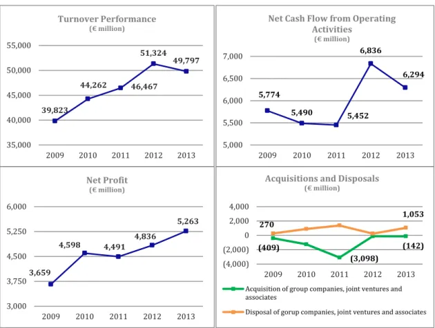
ILLUSTRATION 2 – UNILEVER’S KEY PERFORMANCE INDICATORS (2009-2013)

Source: Unilever’s Annual Reports from 2009 until 2013 and own calculations

From the data showed above, it is perceptible that Unilever has overcome the economic crises. In the past five years, Unilever has shown an annual growth rate of 9.51% on net profit, given that its turnover has increased yearly at a pace of 5.75% and it has been able to take full advantage of its operations since 2011. In addition, the structural changes in terms of acquisitions and disposals of group companies, joint ventures and associates can prove the company has been somewhat investing somewhat, reaching its main value of acquisitions in 2011 (about €3 billion) and profiting few more than €1 billion as disposals last year.

For the purpose of the current Academic Thesis, an equity valuation will be performed on Unilever NV. Therefore, this company will be represented by its publicly traded stock in the Amsterdam Exchange Index – tickers UNA NA and AEX IND, respectively, in Bloomberg. In order to calculate weekly returns of both securities, weekly last prices were taken out from Bloomberg between July of 2009 and July of 2014 (see Appendix 1). In what concerns Unilever’s returns, they have not

39,823 44,262 _46,467 51,324 49,797 35,000 40,000 45,000 50,000 55,000 2009 2010 2011 2012 2013 Turnover Performance (€ million) 5,774 5,490 _5,452 6,836 6,294 5,000 5,500 6,000 6,500 7,000 2009 2010 2011 2012 2013

Net Cash Flow from Operating Activities (€ million) 3,659 4,598 _4,491 4,836 5,263 3,000 3,750 4,500 5,250 6,000 2009 2010 2011 2012 2013 Net Profit (€ million) (409) (3,098) (142) 270 1,053 (4,000) (2,000) 0 2,000 4,000 2009 2010 2011 2012 2013

Acquisitions and Disposals

(€ million)

Acquisition of group companies, joint ventures and associates

(24)

Page | 24 36.3% 27.0% 18.8% 18.0% Personal Care Foods Refreshment Home Care 29.7% 33.3% 19.5% 17.5% Personal Care Foods Refreshment Home Care

suffered major fluctuations during that period, behaving almost the same as its index mainly after July of 2012.

2.2 BUSINESS SEGMENTATION

Being considered one the most successful company within the consumer goods market, it is relevant to discriminate the historical performance between its 4 business segments:

ILLUSTRATION 3 – TURNOVER DISTRIBUTION (2009 VERSUS 2013)

Source: Unilever’s Annual Reports of 2009 and 2013 and own calculations

Analyzing data of 2013, Personal Care (including sales of skin care and hair care products, deodorants and oral care products) is the most important segment given that it is accountable for 36.3% of Unilever’s turnover. Aggregating the Foods segment (including sales of soups, bouillons, sauces, snacks, mayonnaise, salad dressings, margarines and spreads), there are responsible for already 63% of total turnover. Furthermore, when the above structure to the 2009 one, there are no major differences, seeing only a somewhat growth in Personal Care and a slight decrease in Refreshment and Foods segments.

ILLUSTRATION 4 –TURNOVER AND CORE OPERATING PROFIT PER SEGMENT (€M)

Source: Unilever’s Annual Reports from 2009 until 2013 and own calculations

11,846 18,056 13,256 13,426 7,753 9,369 6,968 8,946 5,000 7,500 10,000 12,500 15,000 17,500 20,000 2009 2010 2011 2012 2013

Personal Care Foods

Refreshment Home Care

1,834 3,206 1,840 2,377 731 856 615 577 0 500 1,000 1,500 2,000 2,500 3,000 3,500 4,000 2009 2010 2011 2012 2013

Personal Care Foods

(25)

Page | 25 Regarding now absolute values (as shown in the above graphs) the Personal Care segment is the one with the most visible growth in terms of turnover and core operating profit – around 11% of annual growth rate. All the other segments, have been quite constant, mainly Refreshment (including sales of ice cream, tea-based beverages, weight-management products and nutritionally enhanced staples sold in developing markets) and Home Care (including sales of home care products, such as powders, liquids and capsules, soap bars and a wide range of cleaning products).

2.3 MAIN COMPETITORS

Regarding each business segment, Unilever faces threats as any other company. Nestlé, being the most relevant one since its brand portfolio and respective purposes reach the same market as Unilever, mainly through the sale of Nestea and Nestlé Ice Cream (Refreshment), and Maggi (competing directly with Knorr – Foods).

Furthermore, especially in Home and Personal Care industries, Unilever faces more than one player challenging its products. For instance, the Procter & Gamble Company competes through its Pantene, Head & Shoulders, Fairy and Ariel products. In addition, Henkel, even being one with a smaller brand portfolio, still fights back with its home and hair care products, such as Persil and Schwarzkopf. Beiersdorf is another one but more focused on skin care leading with its well-known Nivea products against Unilever’s Vasenol and Dove. Finally, being almost a home care focused company, Reckitt Benckiser challenges Unilever’s Skip through its brands Calgon and Finish.

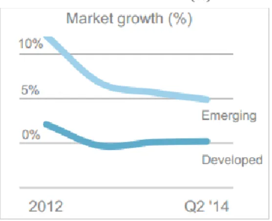
2.4 INDUSTRY INSIGHT

Consumer goods industry, where Unilever is present, is an established mature one. Given that, it is almost unreliable to dream with a large growth in turnover. Nevertheless, due to the economic crisis, consumers purchasing priorities have changed since there is more volatility and uncertainty, leading to an even slower market growth. In the first half of 2014 results presentation, Unilever also adds that according to World Bank, the GDP growth for 2014 will decrease in a worldwide range (except Europe,

which will remain at a constant growth rate – see Appendix 2) resulting in weaker economies. Unilever also accepts the competitiveness within the industry will remain fierce in 2014, leading to a shift of resources into emerging markets and also continuing to make improvements in both processes and products. Moreover, this shift of focus in markets may fight back the lack of growth in the industry, given that it is in a mature phase.

ILLUSTRATION 5 – MARKET GROWTH (%) SINCE 2012

(26)

Page | 26

3 EQUITY VALUATION

3.1 DISCOUNTED CASH FLOW METHODOLOGY

The first Unilever’s equity valuation will be performed under a Discounted Cash Flow perspective. Therefore, the following sections will bring some insight towards the assumptions chosen to forecast relevant variables.

3.1.1 MAIN ASSUMPTIONS

A company’s strategy and managerial decisions impacts its cash flows today and in the near future. Assuming Unilever is under a going concern approach, one needs to determine when all those effects come to an end, reaching afterwards the so called terminal value in perpetuity. Thus, a time frame of 5 years is considered until the terminal value - being after all in accordance to what was referred, in a previous chapter, by Koller et al. (2005).

Moreover, in order to forecast future cash flows, a restructuring needs to be done in the Consolidated Income Statement taking into considerations several assumptions as they will be explained in the following sub-sections.

3.1.1.1 TURNOVER

Since Unilever is a fast-moving consumer goods company, the inflation in consumer prices will be the main variable impacting its turnover. In the 3 years following the economic recession, the annual inflation (worldwide values taken from World Bank Data, since Unilever is a global player) has increased reaching its maximum in 2011 at 5.02%. Successively, it has been re-adjusting itself decreasing to 2.66% last year (see Appendix 3 for historical and future inflation). Since, the era before and after the economic crisis are not the same, I will not take into account the premature values and assume the inflation will remain at a constant rate of 2.66% per year.

ILLUSTRATION 6 – UNILEVER’S TURNOVER THROUGHOUT TIME

Source: Unilever’s Annual Reports, orld Bank Data (inflation rates) and own calculations

48,309 49,592 50,910 52,263 53,652 39,823 44,262 46,467 51,324 _49,797 35,000 40,000 45,000 50,000 55,000

(27)

Page | 27 However, in a more critical manner, the inflation does not have a major impact on consumer behavior in terms of purchasing, given that all products are non-durable ones (promptly consumed) which the price does not have an influent power. Consequently, Unilever might not suffer any impact in terms of volume sales. Nevertheless, given that the consumer goods market is already a mature one, it becomes more difficult for a company to grow.

Furthermore, in 2010, Unilever decided to cut its prices becoming now in need to increase its profit margin. As a result, even though it is in demand to decrease costs, it will behave in accordance to the inflation behavior and increase its prices across every business segment starting in 2014. In fact, in the results for the first half of 2014, the increase in prices has contributed positively at 1.7% for total turnover. Also, the prices change has not negatively affected the volume sales. Instead it has increased 1.9% from last half year.

In addition, having a worldwide presence, exchange rates affects greatly Unilever’s turnover. The following table shows the effect exchange rates have on underlying sales growth (USG) facing the last homologous year:

ILLUSTRATION 7 – EFFECT OF EXCHANGE RATES (%) ON USG 2013 vs.

2012 2012 vs. 2011 2011 vs. 2010 2010 vs. 2009 2009 vs. 2008

Effect of exchange rates (%) (5.9) 2.2 (2.5) 7.3 (2.7)

Source: Unilever’s Annual Reports.

This effect is inconsistent throughout the years only assuming positive impacts every other year and not in the same value. Since 22% of Unilever’s business comes from the United Kingdom, the Netherlands and the United States, a special attention was drawn on the relationship between GBP, EUR and USD. The Appendix 4 shows that the value of EUR facing both GBP and USD has been unstable since the last 5 years, confirming the impact on Unilever’s turnover. Consequently, this variable is extremely difficult to predict in the future, and is not viable to be considered in the analysis.

Furthermore, since first half results of 2014 are already public by the time of the valuation, the turnover behavior during this period will be taken into account as an insight until the end of this year – -5.5% when comparing to the first half of 2013, mainly due to currency movements. As a result, the turnover growth for 2014 will not only depend on the inflation but also on the latter value, leading then to a negative growth of -2.99%. Regarding the following years, it is assumed that Unilever will slowly recover at a constant inflation rate – 2.66%.

ILLUSTRATION 8 – TURNOVER GROWTH RATES (2014-2018)

2014 2015 2016 2017 2018

Turnover Growth (%) (2.99) 2.66 2.66 2.66 2.66

(28)

Page | 28

3.1.1.1.1 TURNOVER ACCORDING TO BUSINESS SEGMENT

The following table represents the distribution of Unilever’s turnover within its 4 segments. The last column shares the compound annual growth rate of each segment’s turnover from 2009 until 2013.

ILLUSTRATION 9 – TURNOVER EVOLUTION ACCORDING TO BUSINESS SEGMENT (%)

Source: Unilever’s Annual Reports and own calculations.

By analyzing Unilever’s turnover structure with its segments, there has been a movement of “strength” from Foods to Personal Care segment, being still the two most profitable segments. ILLUSTRATION 10 – TURNOVER EVOLUTION ACCORDING TO BUSINESS SEGMENT (€M)

The transformation showed in the graph is due to the inflation growth, impacting Unilever as a whole. The assumption to forecast each segment’s turnover is based upon the stability in the turnover distribution already present in 2013 (showed in the table above – 2013 data), meaning there will be no change in the future.

3.1.1.2 COST OF SALES

The assumptions behind the cost of sales forecasting is the same as the one used on turnover – inflation annual rate according to consumer prices. In addition, to forecast the cost of sales, it will be seen as a percentage of the turnover since it has remained somewhat constant (between 58% and 60%) since 2009. Given that 2009 may yet share some residuals from the economic recession, an assumption was made that the cost of sales for future years would be the average of those

2009 2010 2011 2012 2013 CAGR (Absolute values) Personal Care 29.7% 31.1% 33.3% 35.3% 36.3% 11.1% Foods 33.3% 32.0% 30.1% 28.1% 27.0% 0.3% Refreshment 19.5% 19.4% 18.9% 19.0% 18.8% 4.8% Home Care 17.5% 17.5% 17.7% 17.6% 18.0% 6.4% 0 20,000 40,000 60,000

2009 2010 2011 2012 2013 2014E 2015E 2016E 2017E 2018E

(29)

Page | 29 percentages afterwards 2010 (inclusive). At the end, it was reached a fraction of 59.3% of total turnover, used as a constant rate for perpetuity.

Finally, in what concerns the distribution of this variable according to each business segment, the proportions are the same used on the turnover.

3.1.1.3 SELLING AND ADMINISTRATIVE COSTS

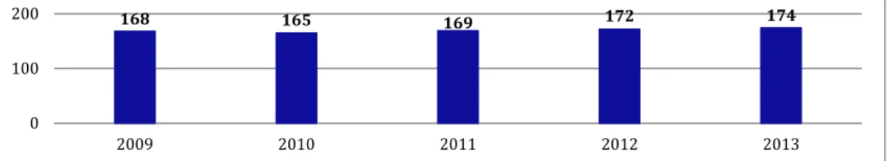
The assumption assumed on forecasting the selling and administrative costs was based upon the average number of employees in the company, as it follows:

ILLUSTRATION 11 – AVERAGE NUMBER OF EMPLOYEES DURING THE YEAR (2009-2013), IN THOUSANDS

Source: Unilever’s Annual Reports.

The graph shows that the staff structure has not suffered any change and its CAGR proves it with 0.88%. Looking at total amounts of selling and administrative costs, I was able to reach unit costs. In this case, the costs per employee have been growing at a yearly rate of 2.01% (CAGR). Using this value, I was able to estimate future unit costs as well for the average number of employees in Unilever, until 2018. Then multiplying these two values led me to the total expenses on selling and administrative costs (see Appendix 6 for restructured income statement).

Since no information regarding this matter accordingly to each segment was shared, the allocation will be performed according to the weight each segment’s gross profit has on the total gross profit.

3.1.1.3.1 RESEARCH AND DEVELOPMENT COSTS

In what concerns the research and development costs, already included in the selling and administrative expenses, they have always been around 2% of Unilever’s turnover. Therefore, this proportion will remain constant towards perpetuity, having consequently no impact on the valuation.

ILLUSTRATION 12 – RESEARCH AND DEVELOPMENT COSTS AS % OF TURNOVER (2009-2013)

168 165 169 172 174 0 100 200 2009 2010 2011 2012 2013 2.1% 2.0% 2.2% 2.1% 2.2% 2013 2012 2011 2010 2009

(30)

Page | 30

3.1.1.4 NET FINANCE COSTS

Regarding net finance costs, these include finance income deducting afterwards finance costs, and pensions and similar obligations. Finance income is estimated assuming that each historical average weight on total earnings before interests and taxes (EBIT) will remain constant throughout time – 1.49%. Whereas, being finance costs more related to the book value of debt, they will change assuming an average weight on total liabilities from last 5 years (1.79%) and liabilities will change according to assumptions made to its items (while estimating net working capital and provisions) – see Appendix 5 for further details.

However, pensions and similar obligations will be dependent on the average number of employees during the year (following the same rationale explained when calculating the selling and administrative costs).

Also, when allocating these values to each segment, it is assumed that both finance income and costs will be proportional to the weight each segment’s EBIT has on total EBIT. On the other hand, since no information is shared regarding the number of employees per business segment, pensions and similar obligations are estimated according to the weight of selling and administrative costs each one has on the whole value (see Appendix 6 for restructured income statement of each business segment).

3.1.1.5 OTHER RESULTS FROM NON-CURRENT INVESTMENTS

In what concerns other results from non-current investments, the behavior is quite difficult to predict and calculating the weight this item has on EBIT (Earnings before Interests and Taxes) confirms it. Leaving behind the year 2009 (given that the weight of 7.3% is too different from the following years), the historical average of this weight is 0.58%, which will be assumed as a constant percentage throughout time. Also, the same assumption is used while allocating values in each Unilever’s segments (considering yearly 0.58% of each EBIT).

3.1.1.6 SHARE OF RESULTS OF JOINT VENTURES & ASSOCIATES

Unilever achieves gains through its participations in joint ventures and associates, needing to state those incomes (or losses) in its Income Statement. In order to forecast these, it was assumed the share of results would depend on the gross profit. Thus, an average of this proportion was calculated using shares of net profits from 2009 until 2013, reaching an average percentage of 0.59%. Consequently, future shares will be 0.59% of estimated gross profit of each year.

The allocation into each business segment is provided in the Annual Report, so the corresponding estimation will be done with last year’s weight of the share of these results on Unilever’s total value.

(31)

Page | 31

3.1.1.7 INCOME TAXES

As stated in Unilever’s Annual Report of 2013, its “effective tax rate remained consistent with 2012 at 26%. Our longer term expectation for the tax rate remains around 26%”. Therefore, the assumption will be made in line with what is expected from the company.

3.1.2 FREE CASH FLOW TO THE FIRM

In the Literature Review, it was mentioned that the enterprise value of a company would be the discounted cash flows of the free cash flow to the firm (FCFF) of each year, following the formula:

(18)

In the following sub-sections, the assumptions used on these variables will be enlightened (see Appendix 8 for complete information regarding calculation of FCFF).

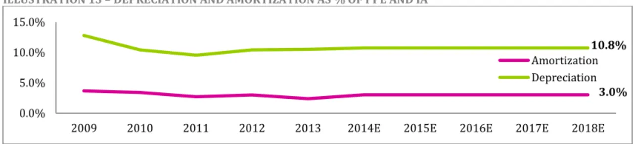
3.1.2.1 DEPRECIATION AND AMORTIZATION

The variables to take into consideration are Depreciation of Property, Plant and Equipment (PPE) and Amortization of Intangible Assets (IA). Therefore, the tendency of these two will be in accordance to historical average of the weight both depreciation and amortization have on PPE and IA. Given that, depreciation is estimated to be 3.0% of forecasted PPE and amortization with 10.8% of IA. In terms of disposals and acquisitions, Unilever is constantly moving and since 2014 is not being an easy one Unilever has sold a few brands in order to not affect so greatly its profits, leaving all open for 2015 and further years. Being that said, future values for both PPE and IA will behave according to Unilever’s turnover.

ILLUSTRATION 13 – DEPRECIATION AND AMORTIZATION AS % OF PPE AND IA

Source: Unilever’s Annual Reports (Balance Sheet and Income Statement) and own calculations.

The disaggregation into business segments is in accordance to the weight each one’s depreciation and amortization had last year on the total amount.

3.0% 10.8% 0.0% 5.0% 10.0% 15.0%

2009 2010 2011 2012 2013 2014E 2015E 2016E 2017E 2018E

Amortization Depreciation

Unilever Group : equity valuation

Equity Valuation

Unilever Group

Candidate:

Susana Pires

152112095

susana.pires@yahoo.com

Supervisor:

Dr. José Carlos Tudela Martins

“UNILEVER: WATCH OUT! TIME TO INVEST”

2014

RECOMMENDATION

BUY

TARGET PRICE

€36.39

ABSTRACT

ACKNOWLEDGMENTS

TABLE OF CONTENTS

1 LITERATURE REVIEW

1.1 INTRODUCTION

1.2 VALUATION MODELS

1.2.1 THE DISCOUNTED CASH FLOWS METHOD

1.2.2 THE ADJUSTED PRESENT VALUE METHOD

1.2.3 RELATIVE VALUATION

1.2.4 OPTION PRICING THEORY AND MODELS

1.2.5 DIVIDEND DISCOUNT MODEL

1.2.6 ECONOMIC VALUE ADDED METHOD

1.2.7 ECONOMIC PROFIT METHOD

1.2.8 VALUATION IN EMERGING MARKETS

1.3 MAIN CONCLUSIONS

1.4 FURTHER CONCERNS

1.4.1 THE TERMINAL VALUE

1.4.2 THE PRESENT VALUE OF THE INTEREST TAX SHIELDS

1.4.3 THE MARKET RISK PREMIUM

1.4.4 LEVERED AND UNLEVERED BETA

1.4.5 COST OF EQUITY

1.4.6 COST OF DEBT

2 UNILEVER

2.1 BRIEF PRESENTATION

2.2 BUSINESS SEGMENTATION

2.3 MAIN COMPETITORS

2.4 INDUSTRY INSIGHT

3 EQUITY VALUATION

3.1 DISCOUNTED CASH FLOW METHODOLOGY

3.1.1 MAIN ASSUMPTIONS

3.1.1.1 TURNOVER

3.1.1.1.1 TURNOVER ACCORDING TO BUSINESS SEGMENT

3.1.1.2 COST OF SALES

3.1.1.3 SELLING AND ADMINISTRATIVE COSTS

3.1.1.3.1 RESEARCH AND DEVELOPMENT COSTS

3.1.1.4 NET FINANCE COSTS

3.1.1.5 OTHER RESULTS FROM NON-CURRENT INVESTMENTS

3.1.1.6 SHARE OF RESULTS OF JOINT VENTURES & ASSOCIATES

3.1.1.7 INCOME TAXES

3.1.2 FREE CASH FLOW TO THE FIRM

3.1.2.1 DEPRECIATION AND AMORTIZATION