Portfolio performance evaluation : the case of the portuguese mutual funds market

WORKING PAPER SERIES

CEEAplA WP No. 14/2009

Portfolio Performance Evaluation: the Case of

the Portuguese Mutual Funds Market

Gualter Couto

Rita Marques Brandão Nuno Roque

Portfolio Performance Evaluation: the Case of the

Portuguese Mutual Funds Market

Gualter Couto

Universidade dos Açores (DEG)

e CEEAplA

Rita Marques Brandão

Universidade dos Açores (DM)

e CEG-IST

Nuno Roque

Universidade dos Açores (DEG)

Working Paper n.º 14/2009

Dezembro de 2009

CEEAplA Working Paper n.º 14/2009 Dezembro de 2009

RESUMO/ABSTRACT

Portfolio Performance Evaluation: the Case of the Portuguese Mutual Funds Market

In this work, we investigate the portfolio performance evaluation of portuguese mutual funds market. For that purpose, we used different models with daily data, where we tested different hypotheses: the existence of alphas with or without selectivity, and the existence of betas with or without timing. There are differences induced by the use of unconditional and conditional models based on non-temporal variation in profitability and risk. The results suggest that fund managers have some capacities of selectivity but not of timing.

JEL classification: G11, G23.

Keywords:Conditional Performance, Mutual Funds, CFG Model, Performance, Selectivity, and Timing.

Gualter Couto

Departamento de Economia e Gestão Universidade dos Açores

Rua da Mãe de Deus, 58 9501-801 Ponta Delgada Rita Marques Brandão

Departamento de Matemática Universidade dos Açores Rua da Mãe de Deus, 58 9501-801 Ponta Delgada Nuno Roque

Departamento de Economia e Gestão Universidade dos Açores

Rua da Mãe de Deus, 58 9501-801 Ponta Delgada

PORTFOLIO PERFORMANCE EVALUATION: THE CASE OF THE

PORTUGUESE MUTUAL FUNDS MARKET

Gualter Couto

Department of Economy and Management, and CEEPLA, University of the Azores, Portugal gcouto@uac.pt

Rita Marques Brandão

Department of Mathematics, University of the Azores, and CEG-IST, Portugal rita@uac.pt

Nuno Roque

Department of Economy and Management, University of the Azores, Portugal nunoroque67@gmail.com

Abstract

In this work, we investigate the portfolio performance evaluation of portuguese mutual funds market. For that purpose, we used different models with daily data, where we tested different hypotheses: the existence of alphas with or without selectivity, and the existence of betas with or without timing. There are differences induced by the use of unconditional and conditional models based on non-temporal variation in profitability and risk. The results suggest that fund managers have some capacities of selectivity but not of timing.

JEL classification:

G11, G23.

Keywords:

Conditional Performance, Mutual Funds, CFG Model, Performance, Selectivity, and Timing.

1 Introduction

From the theoretical point of view the trade off risk versus return has been the main factor to understand the portfolio performance evaluation. The higher the risk of an asset, the higher will be the required premium for assuming that risk, which per si does not mean a better performance evaluation.

The risk variable has been the subject of several studies since the nineteenth-twenties, but it was the work “Portfolio Theory” of Markowitz (1952) that related risk and profitability in a rational way, trying to minimize the risk of the investor to a certain level of expected gain. Sharpe (1964), Lintner (1965) and Mossin (1966), developed a model that describes the relationship between risk and expected return: the Capital Asset Pricing Model (CAPM). The traditional performance approach developed by Jensen (1968) assumes that the risk parameters are constant over the evaluation period. According to the model, the portfolio’s excess of return towards the risk-free rate depends on the parameter beta. Thus, according to Romacho and Cortez (2005), the alpha can be interpreted as the incremental return (positive or negative) obtained in addition to a portfolio under CAPM. To estimate each component of the manager’s contribution to the excess of return, we have the model developed by Treynor and Mazuy (1966) which relates in a non-linear fashion (since they have replaced the linear relationship proposed by the CAPM by a quadratic regression) the portfolio excess of return with the market excess of return. They studied a sample of 57 mutual funds, where they found that the managers have selectivity, but no timing.

One of the conditional measures proposed by Ferson and Schadt (1996) takes into account the portfolio performance evaluation based on investment strategy played by public information. The portfolio performance evaluation of the mutual funds based on the conditional CAPM depends on public information of the macroeconomic variables,

such as: measure of the temporal structure slope of interest rates, dividends growth rate of a market index, indicator of a short-term interest rates, spread between the bond returns of companies with different ratings and a dummy variable for the month of January. These authors assume that the beta of the portfolio is the linear function of the macroeconomic variables vector. Since our investigation is to evaluate the portfolio performance of mutual funds in the portuguese market share, it is worth of notice a study by Cortez and Silva (2002) in which it is used the model of Ferson and Schadt (1996), applied to a sample of 12 funds from national bonds, between April 1994 and March 1998. One verifies that for half of the funds of the sample the alphas are significantly positive. From the implementation of macroeconomic variables results neutral performances.

Christopherson, Ferson and Glassman (1998) created the CFG model, which assumes the existence of a temporal variation of both the conditional betas and alphas. They also apply the portfolio alpha in order to turn it dependable on public information, with macroeconomic mismatching variables, enabling a performance evaluation according to changes in the state of the economy. Christopherson, Ferson and Glassman (1998), conducted an empirical study with a sample of 185 pension funds in the U.S., between 1979 and 1990, and noted the relevance of both betas and alphas with variability over time. In terms of comparison of conditional and unconditional alphas, these are similar, since these funds do not always have large inputs of capital in situations of Bull Market; so that the results of the empirical study are consistent with the interpretation given by Ferson and Schadt (1996).

The purpose of this study is to evaluate and compare the performance of a sample of mutual funds shares of the Portuguese capital market using unconditional and conditional models. The remainder of this paper is organized in four sections. The first

consists of the previous introduction. The second section concerns the methodology which presents the unconditional and conditional models in operational terms. The third section discusses the empirical study, including data, statistics and results. Finally, the fourth section shows the main findings.

2 Methodology

The measure proposed by Jensen (1968) has been taken as a reference for measuring the performance of the portfolio managers. According to Coggins, Beaulieu and Gendron (2004) it is expressed by the following expression:

t c r, = U c α + β_c1r_m,_t +

β

c2Mt+

β

c3uc,t−1 + uc,t (1) where: U c

α

: measure of unconditional performance of the portfolio c;

t c

r_, : excess return (over the risk free rate) of the portfolio c at period ;

t

1

c

β

: measure of market risk of the portfolio c;

t m

r _, : market premium over the period ;t

2

c

β

: parameter associated with the weekend effect of the portfolio ;c

t

M : binary variable that takes the value 1 on the first day of the week and 0 for the remaining days of the week;

3

c

β

: coefficient related to the moving average model of order 1 term for the portfolio ;c and

1 ,t−

c

Expression (1) takes into consideration that the level of risk of the portfolio remains constant over time. So

α

cU means the incremental return from beyond the profitability

at the level of market risk assumed.

The CFG model proposed by Christopherson, Ferson and Glassman (1998) assumes the existence of a temporal variation of both the conditional betas and alphas. In this paper we apply the model adapted by Coggins, Beaulieu and Gendron (2004). The model takes the form:

t c r_, =

α

_cCFG+A′_cz_t−1 +b0_cmr_m,_t+B′cm

(

zt−1rm,t

)

+

β

c2Mt+

β

c3uc,t−1+uc,t (2) where: CFG c

α

: average alpha of the portfolio ;c

: 1 −

t

z vector representing the difference between the realization of the public information variables and their unconditional average; :

c

A′ vector that measures the response of the conditional alpha of the portfolio cto the information variables;

cm

b₀ : average beta (the unconditional mean of the conditional beta) of

the portfolio ;c

:

cm

B′ vector that measures the response of the conditional beta of the portfolio cto the information variables;

the remaining variables were previously defined.

In order to investigate the abilities of the portfolio managers to anticipate market movements, we added the quadratic term r_m2_,t to equations (1) and (2) as in Mazuy and Treynor (1966).

The unconditional model (1) becomes:

t c r_, =

α

cU2+

β

c1rm,t + 2 , 2 4 mt U c r

β

+

β

c2Mt+

β

c3uc,t−1 + uc,t (3)

and the CFG based model (2) becomes: t c r_, =

α

cCFG2+A′czt−1+b0cmrm,t+B′cm

(

zt−1rm,t

)

+ 2 , 2 4 mt CFG c r

β

+

β

c2Mt+

β

c3uc,t−1+uc,t (4)

If the values of

α

_cU2 and

α

_cCFG2 are significant and positive then the portfolio managers abilities to select securities is improved (selectivity ability). A significantly positive

2 4

U c

β

and

β

cCFG₄ 2 indicates that these managers change their exposure to risk in order to

increase its profitability (timing ability).

3 Empirical Study

The period of this research study is from January 2003 to December 2006. We used daily data, corresponding to 994 records for each fund. Our study is composed by 10 Portuguese mutual funds, domiciled in the portuguese market, and classified according to the criteria’s of the Associação Portuguesa de Fundos de Investimento, Pensões e

Patrimónios (PAIFPH) and Fundos de Acções Nacionais (FAN). The FAN invest at least 2/3 of the portfolio in shares (aggressive funds), with assets in Euro currency and issued by national authorities. The mutual funds data were obtained from the Comissão

de Mercado de Valores Mobiliários (CMVM) and from the Sociedades Gestoras de

Fundos de Investimento Mobiliário (SGFIM).

In Table 1 we present the name of the mutual funds analysed in this study. (insert Table 1)

In this study we used three macroeconomic variables or conditional variables: the return rate for the dividend of the market index, the slope of the temporal structure of interest rates and a short-term interest rate. The return rate for the dividend of the market index is calculated based on the Portuguese Stock Index Total Return (PSI₂₀TR). The slope of

the temporal structure of interest rates was found from the difference between the returns of two treasury bonds, a long-term and other short-term. The return of the Treasury bond is also used as an indicator for the macroeconomic variable short-term interest rate, as well as the risk free rate.

The daily return on the capital market is based on the PSI₂₀TR.

The determination of the market return is made according to the following formula and the data for it were obtained from Euronext Lisbon:

t m R _, = ln _       −TR PSI TR PSI t t 1 20 20 (5) where: t m

R _, : daily return of the capital market in the period t under the index

; 20 TR PSI TR PSI t

20 : index value of the capital market in the period ;t and :

1

20 TR

PSI

t− index value of the capital market in the period t−1.

The data required to calculate the returns of the portfolios (funds) were obtained from the CMVM and the SGFIM.

The total return of the portfolio (fund) c in the period t is calculated as follows:

t c R_, = ln _       −1 , , t c t c UP UP (6) where: t c

UP_, : price for the portfolio (fund) c at the end of period t ; and

1 ,t−

c

UP : price for the portfolio (fund) c at the end of period t−1.

In this study we also included a dummy variable that tests the “Monday effect”. This variable takes value 1 on this day and for the remaining days of the week value 0.

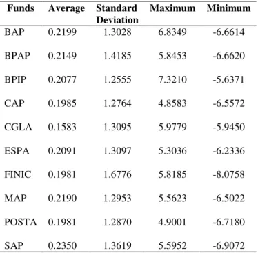
The summary statistics of the funds returns are presented in Table 2. (insert Table 2)

The parameters estimates obtained through the equations (1) to (4), for each performance measure, are presented below. The parameters of each model were estimated by maximum likelihood method using SPSS version 15.0.

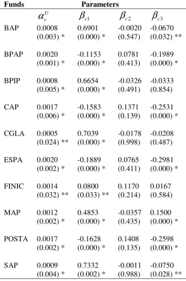
Table 3 presents the results of the unconditional model (1). (insert Table 3)

Considering the period in analysis, the results indicate that fund managers have little capacity to outperform the market. The estimates of U

c

α

are positive, but very close to zero. Eight estimates of

α

cU (BAP, BPAP, BPIP, CAP, ESPA, MAP, SAP and POSTA)

are statistically significant at level 1% and two (CGLA and FINIC) at level 5%.

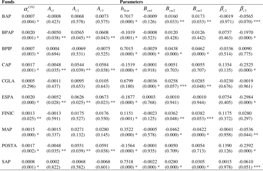
The estimated parameters obtained through the CFG based model are indicated in Table 4.

(insert Table 4)

In this case, the conditional alpha measure suggests a neutral performance of the fund managers (positive alphas but very close to zero). The same eight funds have statistically significant

α

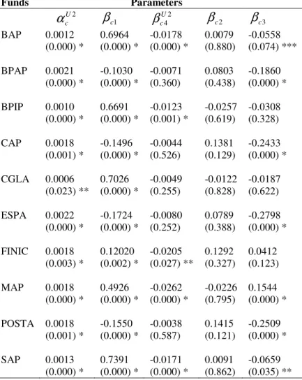
_cCFGat level 1% and one fund (FINIC) at level 5%. The estimate of CGLA is not significant.

Estimates of parameters obtained from equation (3), allows us to analyze the selectivity and timing abilities based on the Treynor and Mazuy (1966) parameterization with unconditional market risk.

(insert Table 5)

According to the results in Table 5, it is notorious that the fund managers present some capacity of selectivity. The values of

α

_cU2 are positive; however they are very close to

present positive significant values of

α

U_c2 at level 1% and the fund CGLA at level 5%. On the other hand, we observe that the managers are incapable to anticipate market developments since the values of

β

_cU₄2 in all funds are negative. Only five funds (BAP, BPIP, FINIC, MAP and SAP) have statistical significant values.

Finally the analysis of selectivity and timing using the CFG based model and the Treynor and Mazuy (1966) performance measure is summarized in Table 6.

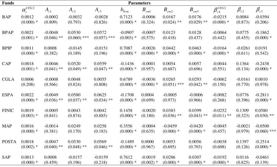
(insert Table 6)

Again we can observe that the fund managers show some selection ability (the values of 2

CFG

α are very close to zero). The estimated values of β_cCFG₄ 2(timing component) lead us to the conclusion that there is no capacity from the managers to anticipate market developments. With the exception of the fund CGLA (with a non significant estimate value of αCFG2) all others present positive and statistically significant values at level 1%.

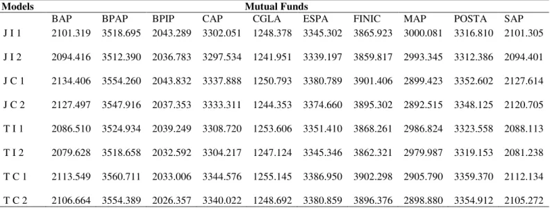
For the timing component, four funds (BAP, BPIP, FINIC and SAP) are negative and statistically significant. The others are also negative but without statistical significance. The results presented in tables 3, 4, 5 and 6 show that the variable weekend effect has no statistical significance in any measure and in any mutual fund. Therefore, we decided to compare the models with and without the variable “weekend effect” to investigate if there is an improvement in the models by excluding this variable. The results that were obtained are reported in Table 7. According to Schwarz‘s Bayesian Criterion (BIC) the models without the presence of the variable “weekend effect” are the best (smaller value of BIC).

4 Conclusion

The values of the 10 Portuguese mutual funds have some ability of selectivity (insignificant) for being extremely close to zero for the 4 measures used. Still, in terms of Jensen's alpha (1968) parameterization with unconditional market risk, the best performance is the BPAP and the ESPA. As for the conditional alpha of Jensen (1968) second CFG, the BPAP and ESPA show the best result. The empirical application of the model of Treynor and Mazuy (1966) parameterization with unconditional market risk, indicates that ESPA has better performance. Finally the model of Treynor and Mazuy (1966) CFG second, gives us indication that the ESPA offers the best result. In terms of timing, no mutual fund presents figures showing the managers’ ability in predicting the market’s development. This happens in both the unconditional and the conditional measure. The found results in terms of selectivity using the unconditional parameterization and CFG with daily data are in part similar to those in the literature that also uses these parameterizations, with monthly data. Regarding the timing it was still not possible to find the unconditional parameterization and CFG with daily data, as in the literature with monthly data.

References

Christopherson, J., Ferson, W., and Glassman, D. (1998). Conditioning Manager Alphas on Economic Information: Another Look at the Persistence of Performance. Review of

Financial Studies, 11 (1), 111-142.

Coggins, F., Beaulieu, M. C., and Gendron, M. (2004). Mutual Fund Daily Conditional Performance: Selectivity and Timing Measurements. Working Paper, Laval University, Faculty of the Sciences of Administration and Sherbrooke University, Faculty of the Sciences of Administration.

Cortez, M.C., and Silva, F. (2002). Conditioning Information on Portfolio Performance Evaluation: A Reexamination of Performance Persistence in The Portuguese Mutual Fund Market. Finance India, 16 (4), 1393-1408.

Jensen, M. (1968). The Performance of Mutual Funds in the Period 1945-1964.Journal

of Finance, 23 (2), 389-416.

Lintner, J. (1965). The Valuation of Risk Assets and the Selection of Risky Investments in Stock Portfolios and Capital Budgets. Review of Economics and Statistics, 47 (1), 13-37.

Markowitz, H. (1952). Portfolio Selection. Journal of Finance, 7 (1), 77-91.

Mossin, J. (1966). Equilibrium in a Capital Asset Market. Econometrica, 34 (4), 768-783.

Romacho, J.C., and Cortez, M.C. (2005). Os Gestores de Carteiras têm Capacidade de Selecção de Títulos e de Previsão da Evolução do Mercado? Um Estudo Empírico para o Mercado Português. Tékhne-Revista de Estudos Politécnicos, 2 (4), 39-58. Schwarz, G. (1978). Estimating the Dimension of a Model. Annals of Statistics, 6 (2),

461-464.

Sharpe, W. (1964). Capital Asset Prices: a Theory of Market Equilibrium Under Conditions of Risk. Journal of Finance, 19 (3), 425-442.

Treynor, J., and Mazuy, K. (1966). Can Mutual Funds Outguess the Market? Harvard

Tables

Table 1 - Mutual Funds

Table 2 - Summary statistics of the funds returns.

Funds of National Shares

Banif Acções Portugal (BAP)

Barclays Premier Acções Portugal (BPAP) BPI Portugal (BPIP)

Caixagest Acções Portugal (CAP) Caixagest Gestão Lusoacções (CGLA) Espírito Santo Portugal Acções (ESPA) Finicapital (FINIC)

Millennium Acções Portugal (MAP) Postal Acções (POSTA)

Santander Acções Portugal (SAP)

Funds Average Standard Deviation Maximum Minimum BAP 0.2199 1.3028 6.8349 -6.6614 BPAP 0.2149 1.4185 5.8453 -6.6620 BPIP 0.2077 1.2555 7.3210 -5.6371 CAP 0.1985 1.2764 4.8583 -6.5572 CGLA 0.1583 1.3095 5.9779 -5.9450 ESPA 0.2091 1.3097 5.3036 -6.2336 FINIC 0.1981 1.6776 5.8185 -8.0758 MAP 0.2190 1.2953 5.5623 -6.5022 POSTA 0.1981 1.2870 4.9001 -6.7180 SAP 0.2350 1.3619 5.5952 -6.9072

Table 3 - Estimates of the unconditional model t c r_, = α_cU+ β_c1r_m,t + β_c2M_t+ β_c3u_c,t−1 + u_c,_t Funds Parameters U c α βc1 βc2 βc3 BAP 0.0008 (0.003) * 0.6901 (0.000) * -0.0020 (0.547) -0.0670 (0.032) ** BPAP 0.0020 (0.001) * -0.1153 (0.000) * 0.0781 (0.413) -0.1989 (0.000) * BPIP 0.0008 (0.005) * 0.6654 (0.000) * -0.0326 (0.491) -0.0333 (0.854) CAP 0.0017 (0.006) * -0.1583 (0.000) * 0.1371 (0.139) -0.2531 (0.000) * CGLA 0.0005 (0.024) ** 0.7039 (0.000) * -0.0178 (0.998) -0.0208 (0.487) ESPA 0.0020 (0.002) * -0.1889 (0.000) * 0.0765 (0.411) -0.2981 (0.000) * FINIC 0.0014 (0.032) ** 0.0800 (0.033) ** 0.1170 (0.214) 0.0167 (0.584) MAP 0.0012 (0.002) * 0.4853 (0.000) * -0.0357 (0.435) 0.1500 (0.000) * POSTA 0.0017 (0.002) * -0.1628 (0.000) * 0.1408 (0.135) -0.2598 (0.000) * SAP 0.0009 (0.004) * 0.7332 (0.002) * -0.0011 (0.988) -0.0750 (0.028) ** *- 1% level of significance ** - 5% level of significance *** - 10% level of significance

Table 4 - Estimates of the conditional model t c r_, = α_cCFG+A_c′z_t−1 +b_0cmr_m,t+B′_cm

(

z_t−1r_m,t

)

+

β

_c2M_t+

β

_c3u_c,_t−1+uc,t. Funds Parameters CFG c α Ac1 Ac2 Ac3 b0cm Bcm1 Bcm2 Bcm3

β

c2

β

c3 BAP 0.0007 (0.004) * -0.0008 (0.423) 0.0068 (0.578) 0.0073 (0.575) 0.7017 (0.000) * -0.0009 (0.126) 0.0160 (0.033) ** 0.0173 (0.033) ** -0.0019 (0.971) -0.0565 (0.070) *** BPAP 0.0020 (0.001) * -0.0050 (0.038) ** 0.0565 (0.045) ** 0.0608 (0.043) ** -0.1019 (0.001) * -0.0008 (0.523) 0.0120 (0.428) 0.0126 (0.442) 0.0757 (0.463) -0.1970 (0.000) * BPIP 0.0007 (0.003) * 0.0004 (0.694) -0.0069 (0.531) -0.0075 (0.525) 0.7015 (0.000) * -0.0029 (0.000) * 0.0438 (0.000) * 0.0462 (0.000) * -0.0336 (0.514) 0.0090 (0.775) CAP 0.0017 (0.001) * -0.0048 (0.035) ** 0.0544 (0.039) ** 0.0584 (0.038) ** -0.1519 (0.000) * -0.0001 (0.918) 0.0051 (0.703) 0.0055 (0.707) 0.1354 (0.135) -0.2525 (0.000) * CGLA 0.0005 (0.296) -0.0011 (0.437) 0.0095 (0.653) 0.0105 (0.643) 0.6799 (0.180) -0.0036 (0.000) * 0.0258 (0.057) *** 0.0285 (0.048) ** -0.0230 (0.676) -0.0019 (0.961) ESPA 0.0020 (0.000) * -0.0052 (0.028) ** 0.0626 (0.025) ** 0.0673 (0.023) ** -0.1877 (0.000) * 0.0003 (0.768) -0.0010 (0.941) -0.0010 (0.944) 0.0754 (0.405) -0.2984 (0.000) * FINIC 0.0013 (0.025) ** -0.0013 (0.591) 0.0175 (0.527) 0.0176 (0.550) 0.1151 (0.001) * -0.0023 (0.125) 0.0362 (0.048) ** 0.0382 (0.053) *** 0.1175 (0.372) 0.0280 (0.297) MAP 0.0015 (0.000) * -0.0015 (0.337) 0.0271 (0.132) 0.0280 (0.145) 0.3522 (0.000) * -0.0005 (0.578) -0.0462 (0.000) * -0.0422 (0.000) * -0.0041 (0.958) -0.0536 (0.044) ** POSTA 0.0017 (0.002) * -0.0048 (0.035) ** 0.0551 (0.039) ** 0.0591 (0.038) ** -0.1564 (0.000) * -0.0001 (0.935) 0.0050 (0.709) 0.0054 (0.713) 0.1390 (0.126) -0.2592 (0.000) * SAP 0.0008 (0.001) * 0.0002 (0.822) -0.0068 (0.582) -0.0068 (0.601) 0.7518 (0.000) * -0.0022 (0.000) * 0.0280 (0.000) * 0.0305 (0.000) * 0.0015 (0.978) -0.0610 (0.051) *** *- 1% level of significance ** - 5% level of significance

Table 5 - Analysis of selectivity and timing using the unconditional model model and the Treynor and Mazuy (1966) performance measure

t c r_, = αU_c2+ β_c1r_m,t +

β

_cU₄2r_m2_,t + β_c2M_t+β_c3u_c,t−1 + u_c,t. Funds Parameters 2 U c α βc1 2 4 U c β βc2 βc3 BAP 0.0012 (0.000) * 0.6964 (0.000) * -0.0178 (0.000) * 0.0079 (0.880) -0.0558 (0.074) *** BPAP 0.0021 (0.000) * -0.1030 (0.000) * -0.0071 (0.360) 0.0803 (0.438) -0.1860 (0.000) * BPIP 0.0010 (0.000) * 0.6691 (0.000) * -0.0123 (0.001) * -0.0257 (0.619) -0.0308 (0.328) CAP 0.0018 (0.001) * -0.1496 (0.000) * -0.0044 (0.526) 0.1381 (0.129) -0.2433 (0.000) * CGLA 0.0006 (0.023) ** 0.7026 (0.000) * -0.0049 (0.255) -0.0122 (0.828) -0.0187 (0.622) ESPA 0.0022 (0.000) * -0.1724 (0.000) * -0.0080 (0.252) 0.0789 (0.388) -0.2798 (0.000) * FINIC 0.0018 (0.003) * 0.12020 (0.002) * -0.0205 (0.027) ** 0.1292 (0.327) 0.0412 (0.123) MAP 0.0018 (0.000) * 0.4926 (0.000) * -0.0262 (0.000) * -0.0226 (0.795) 0.1544 (0.000) * POSTA 0.0018 (0.001) * -0.1550 (0.000) * -0.0038 (0.587) 0.1415 (0.121) -0.2509 (0.000) * SAP 0.0013 (0.000) * 0.7391 (0.000) * -0.0171 (0.000) * 0.0091 (0.862) -0.0659 (0.035) ** *- 1% level of significance ** - 5% level of significance *** - 10% level of significance

Table 6 - Analysis of the selectivity and timing using the CFG based model and the Treynor and Mazuy (1966) performance measure t c r_, = α_cCFG2+A′_cz_t−1+b_0cmr_m,t+B′_cm

(

z_t−1r_m,t

)

+

β

_cCFG₄ 2r_m2_,t +

β

_c2M_t+

β

_c3u_c,t−1+u_c,t. Funds Parameters 2 CFG c α Ac1 Ac2 Ac3 b0cm Bcm1 Bcm2 Bcm3 2 4 CFG c β

β

c2

β

c3 BAP 0.0012 (0.000) * -0.0002 (0.809) -0.0032 (0.793) -0.0028 (0.826) 0.7123 (0.000) * -0.0006 (0.324) 0.0167 (0.024) ** 0.0176 (0.029) ** -0.0215 (0.000) * 0.0084 (0.873) -0.0394 (0.206) BPAP 0.0021 (0.001) * -0.0048 (0.046) ** 0.0530 (0.060) *** 0.0572 (0.057) *** -0.0907 (0.003) * -0.0007 (0.575) 0.0123 (0.418) 0.0128 (0.437) -0.0064 (0.442) 0.0775 (0.455) -0.1862 (0.000) * BPIP 0.0011 (0.000) * 0.0008 (0.382) -0.0145 (0.189) -0.0151 (0.196) 0.7087 (0.000) * -0.0026 (0.000) * 0.0442 (0.000) * 0.0463 (0.000) * -0.0164 (0.000) * -0.0261 (0.611) 0.0191 (0.542) CAP 0.0018 (0.001) * -0.0046 (0.041) ** 0.0520 (0.049) ** 0.0559 (0.047) ** -0.1436 (0.000) * -0.0001 (0.957) 0.0054 (0.687) 0.0057 (0.696) -0.0044 (0.551) 0.1364 (0.134) -0.2438 (0.000) * CGLA 0.0006 (0.208) -0.0008 (0.566) 0.0048 (0.824) 0.0055 (0.808) 0.6789 (0.000) * -0.0036 (0.000) * 0.0265 (0.051) *** 0.0293 (0.042) ** -0.0062 (0.150) -0.0161 (0.770) 0.0010 (0.978) ESPA 0.0022 (0.000) * -0.0049 (0.036) ** 0.0580 (0.037) ** 0.0625 (0.034) ** -0.1708 (0.000) * 0.0004 (0.699) -0.0005 (0.973) -0.0006 (0.966) -0.0082 (0.268) 0.0776 (0.396) -0.2811 (0.000) * FINIC 0.0019 (0.003) * -0.0005 (0.841) 0.0043 (0.874) 0.0042 (0.885) 0.1458 (0.000) * -0.0020 (0.180) 0.0383 (0.036) ** 0.0399 (0.043) ** -0.0252 (0.011) ** 0.1309 (0.323) 0.0580 (0.030) ** MAP 0.0016 (0.000) * -0.0014 (0.381) 0.0249 (0.170) 0.0258 (0.183) 0.3556 (0.000) * -0.0004 (0.635) -0.0459 (0.000) * -0.0420 (0.000) * -0.0045 (0.457) -0.0021 (0.979) -0.0500 (0.060) *** POSTA 0.0018 (0.002) * -0.0047 (0.040) ** 0.0530 (0.048) ** 0.0569 (0.046) ** -0.1489 (0.000) * 0.0000 (0.967) 0.0053 (0.695) 0.0056 (0.703) -0.0038 (0.608) 0.1397 (0.126) -0.2514 (0.000) * SAP 0.0013 (0.000) * 0.0008 (0.459) -0.0157 (0.196) -0.0159 (0.218) 0.7612 (0.000) * -0.0019 (0.002) * 0.0286 (0.000) * 0.0307 (0.000) * -0.0192 (0.000) * 0.0116 (0.825) -0.0461 (0.139) *- 1% level of significance ** - 5% level of significance

Table 7 – Comparison of models by the Schwarz’s Bayesian Criterion (BIC).

Models Mutual Funds

BAP BPAP BPIP CAP CGLA ESPA FINIC MAP POSTA SAP

J I 1 2101.319 3518.695 2043.289 3302.051 1248.378 3345.302 3865.923 3000.081 3316.810 2101.305 J I 2 2094.416 3512.390 2036.783 3297.534 1241.951 3339.197 3859.817 2993.345 3312.386 2094.401 J C 1 2134.406 3554.260 2043.832 3337.888 1250.793 3380.789 3901.406 2899.423 3352.602 2127.614 J C 2 2127.497 3547.916 2037.353 3333.311 1244.353 3374.660 3895.302 2892.515 3348.125 2120.705 T I 1 2086.510 3524.934 2039.249 3308.720 1253.606 3351.410 3868.261 2986.824 3323.558 2088.113 T I 2 2079.628 3518.658 2032.592 3304.217 1247.124 3345.346 3862.321 2979.987 3319.153 2081.238 T C 1 2113.549 3560.711 2033.006 3344.576 1255.145 3386.950 3902.298 2905.790 3359.370 2112.134 T C 2 2106.664 3554.389 2026.357 3340.022 1248.692 3380.859 3896.376 2898.880 3354.912 2105.272

Legend: J I 1 – Jensen Unconditional with variable weekend effect. J I 2 – Jensen Unconditional without variable weekend effect. J C 1 – Jensen Conditional with variable weekend effect. J C 2 – Jensen Conditional without variable weekend effect. T I 1 – Treynor Unconditional with variable weekend effect. T I 2 – Treynor Unconditional without variable weekend effect. T C 1 – Treynor Conditional with variable weekend effect. T C 2 – Treynor Conditional without variable weekend effect.