BUSINESS CYCLE DYNAMICS ACROSS EUROPE:
A CLUSTER ANALYSIS
Daniel Fernandes Gonçalves
Dissertation submitted as partial requirement for the conferral of Master in Economics
Supervisor:
Prof. Doutor Luís Filipe Martins, Assistant Professor, ISCTE-IUL Department of Quantitative Methods for Management and Economics
Co-supervisor:
PhD Candidate Rui Silva, University of Milan, Department of Economics, Management and Quantitative Methods
This dissertation aims to analyze the dynamics of business cycles across European coun-tries between 1960Q1 and 2016Q1. For such purpose we identify country-groups of national
deviation cycles through Hierarchical Agglomerative Clustering with the Ward’s method. The clustering technique suggests the existence of three country-groups, which include,
aside from other countries, France and Spain in Cluster 1, United Kingdom and Denmark in Cluster 2 and Germany and Italy in Cluster 3. We execute an extensive analysis on
business cycle stylized facts, synchronization and turning points detection over the clus-ters’ deviation cycles. Further on, we analyze the propagation of economic shocks through
a VAR model, over which we study Granger-causalities, Impulse Response Functions and Forecast Error Variance Decomposition.
Our results show that both Cluster 1 and Cluster 2 share similar cyclical character-istics when compared to Cluster 3. Nevertheless, Cluster 1 and Cluster 3 appear to be
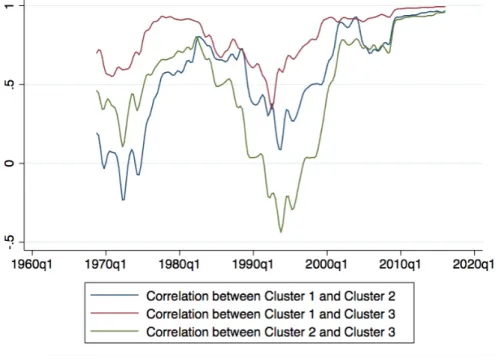
the most synchronous pair, and simultaneously verify the largest proportion of time spent in the same cyclical phase. We show that there has been an increasing business cycle
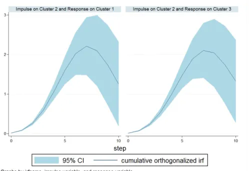
synchronization in Europe since the beginning of the 90’s. The structural analysis shows that Cluster 1 and Cluster 2 have the strongest permanent cumulative shocks, whereas
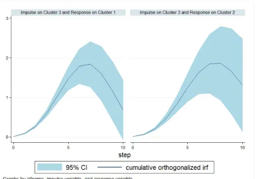
Cluster 3 induces not only the weakest impulses but also explains the smallest fraction of the counterparts’ forecast error variance decomposition. These conclusions question the
"German Dominance" hypothesis and allow the identification of alternative major economic propellers in Europe.
JEL Classification: E32, E37
Key words: Business Cycle stylized facts and synchronization; Hierarchical
A presente tese pretende analisar as dinâmicas dos ciclos económicos na Europa no período compreendido entre 1960Q1 e 2016Q1. Como tal, procedemos à identificação de
grupos de ciclos económicos nacionais através de Clusterização Hierárquica Aglomerativa com o método de Ward. A Clusterização sugere a existência de três grupos que incluem,
além de outros países, França e Espanha no Cluster 1, Reino Unido e Dinamarca no Cluster 2, e Alemanha e Itália no Cluster 3. Analisamos as principais características, sincronização
e cronologia de pontos de inflexão dos ciclos económicos dos clusters. Estudamos ainda a propagação de choques económicos com um modelo VAR, sobre o qual concluímos sobre
causalidade à Granger, funções de impulso-resposta e decomposição de variância.
Os resultados mostram que o Cluster 1 e Cluster 2 apresentam maiores semelhanças
nas características dos seus ciclos quando comparados ao Cluster 3. Simultaneamente, o Cluster 1 e Cluster 3 apresentam quer o maior nível de sincronização quer a maior fração de
tempo partilhada na mesma fase cíclica. Concluímos também que o nível de sincronização dos ciclos económicos na Europa apresenta uma tendência crescente, especialmente após
os anos 90. A análise estrutural conclui que o Cluster 1 e Cluster 2 produzem os choques permanentes mais fortes, enquanto que o Cluster 3 induz os impulsos mais fracos, além
de explicar a menor parte da decomposição de variância do erro de previsão dos restantes. As presentes conclusões questionam a hipótese de "Domínio Alemão" e permitem a
identi-ficação de outros propulsores económicos na Europa.
Classificação JEL: E32, E37
Palavras-Chave: Sincronização de Ciclos Económicos; Técnicas de Clusterização
Hi-erárquica Aglomerativa; Funções Impulso-Resposta; Erros de Previsão e Decomposição de
In the first place, I thank Professor Luís Martins for the guidance, suggestions and help throughout the development of this dissertation.
To Rui Silva, for the long conversations, discussions and shares of thoughts. I especially
thank him for all the dedication, persistence, resilience and patience, that proved to be the most important in all aspects. Grazie per tutto my dear friend!
To Kina and Kiko, for all their love and kindness. The real meaning of life to me is present
in their words, pursuits and dreams. From the bottom of my hearth I thank them, with these simple pages, for all the efforts that they have made for me.
To Jéssica, for the unconditional presence, support and love. For all the words and shared
dreams. May I have all of you in everyday of my life. 273
To all my family, here and abroad, that always stand by my side. Ensemble, ma petite rose!
And finally to André and all my friends, from kindergarten to ISCTE, from Vienna to Washington D.C., for the all the experiences and lifetime memories.
1 Introduction 1
2 Literature Review 3
2.1 Business Cycle Theories . . . 3
2.1.1 From the Classicals to the Austrian School of Thought . . . 3
2.1.2 Schumpeter’s Revolutionary Business Cycle Scheme . . . 5
2.1.3 The behavior of economic agents and its implications on Business Cycles . . . 6
2.1.4 The Real Business Cycle . . . 8
2.2 Business Cycle Dynamics in Europe . . . 9
2.2.1 Business Cycle Synchronization in Industrialized Countries . . . 9
2.2.2 Major Institutional Events in Europe and Business Cycle Synchro-nization . . . 10
2.3 Shocks and propagation mechanisms . . . 13
2.4 Core-Periphery aggregations and country-clusters analysis . . . 15
3 Methodology 19 3.1 Hierarchical Agglomerative Clustering . . . 19
3.2 Turning Points Dating and Business Cycle metrics . . . 20
3.3 Econometric Framework . . . 24
4 Data and Business Cycle Estimation 27 5 Empirical Findings 30 5.1 Cluster Analysis . . . 30
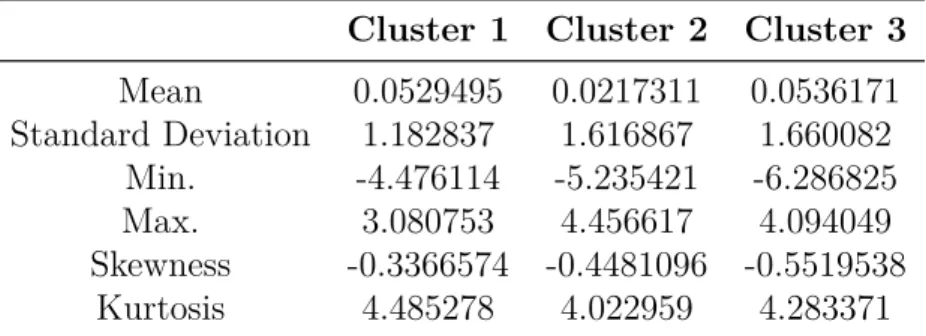
5.2 Stylized facts of the Deviation Cycles . . . . 35
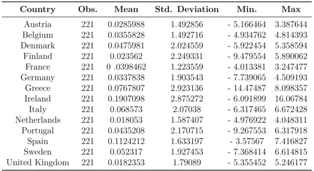
5.2.1 Descriptive Statistics . . . 35
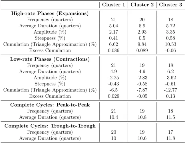
5.2.2 Dissecting the Deviation Cycles . . . . 37
5.3.2 Granger-causality . . . 48
5.3.3 IRF and FEVD analysis . . . 48
6 Concluding Remarks 55 References 58 A Appendices 72 A.1 Descriptive Statistics . . . 72
A.2 Cross-Correlations between National Deviation Cycles . . . . 73
A.3 Stationarity Tests . . . 74
A.4 Graphical representation of Domestic time-series . . . 75
A.5 MATLAB routine for HAC analysis . . . 76
A.6 Stationarity Tests for the identified Clusters . . . 76
A.7 Econometric Framework for Cluster 1 VAR Model . . . 77
A.8 Econometric Framework for Cluster 2 VAR Model . . . 80
A.9 Econometric Framework for Cluster 3 VAR Model . . . 82
A.10 Turning Points, Phases and Cycles per Cluster Deviation Cycle . . . 84
A.11 Statistical Significance for the Index of Concordance . . . 87
A.12 Econometric Framework for all Clusters VAR Model . . . 88
A.13 FEVD for all Clusters VAR Model . . . 91
List of Figures
Figure 1 Dendrogram for Hierarchical Agglomerative Clustering with Ward’s method . . . 31Figure 2 Geographical location of the identified Clusters . . . 33
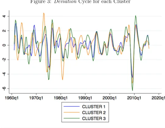
Figure 3 Deviation Cycle for each Cluster . . . 41
Figure 7 Impulse on Cluster 3 IRF and responses on Cluster 1 and Cluster 2 52 Figure 8 Graphical representation of the National Business Cycles (GDP
Quar-terly Growth, Cyclical Component and Trend Component) . . . 75 Figure 9 National Business Cycles in Cluster 1 . . . 77
Figure 10 Roots of the Companion Matrix for Cluster 1 VAR Model (6 lags) . 78 Figure 11 National Business Cycles in Cluster 2 . . . 80
Figure 12 Roots of the Companion Matrix for Cluster 2 VAR Model (8 lags) . 81 Figure 13 National Business Cycles in Cluster 3 . . . 82
Figure 14 Roots of the companion matrix for the 3 Clusters’ VAR model (13 lags) . . . 88
Figure 15 Roots of the companion matrix for all Clusters VAR (7 lags) . . . . 90 Figure 16 Impulse on Cluster 1: FEVD for Cluster 2 and Cluster 3 . . . 91
Figure 17 Impulse on Cluster 2: FEVD for Cluster 1 and Cluster 3 . . . 92 Figure 18 Impulse on Cluster 3: FEVD for Cluster 1 and Cluster 2 . . . 92
List of Tables
Table 1 Some Literature Review on Business Cycle Cluster Analysis . . . 18
Table 2 Deviation Cycle Characteristics per Cluster . . . 36 Table 3 Business Cycle Characteristics in cycles and phases per Cluster
devi-ation cycle . . . . 38 Table 4 Relationship Amplitude-Duration per phase . . . 40
Table 5 Synchronization Metrics: Cross-Correlations and Index of Concordance 43 Table 6 Descriptive Statistics for Domestic deviation cycles . . . . 72
Table 7 Cross-Correlations between National Business Cycles . . . 73 Table 8 ADF Test Results for Domestic Quarterly GDP Growth series . . . 74
(lag 1-10) . . . 77
Table 12 Granger Causality for Cluster 1 VAR Model (6 lags) . . . 79
Table 13 Lagrange-Multiplier test for Autocorrelation in Cluster 1 (lag 1 to 6) 79 Table 14 Optimum Lag Criteria - VAR for Cluster 2 National Business Cycles 80 Table 15 Granger Causality after Cluster 2 VAR Model (8 lags) . . . 81
Table 16 Lagrange-Multiplier test for Autocorrelation for Cluster 2 VAR Model (8 lags) . . . 82
Table 17 Optimum Lag Criteria - VAR for Cluster 3 National Business Cycles 83 Table 18 Granger Causality for Cluster 3 National Business Cycles VAR . . . 83
Table 19 Lagrange-Multiplier test for Autocorrelation in Cluster 3 National Business Cycles VAR . . . 84
Table 20 List of Turning Points . . . 84
Table 21 List of Phases and Cycles for Cluster 1 Deviation Cycle . . . . 85
Table 22 List of Phases and Cycles for Cluster 2 Deviation Cycle . . . . 86
Table 23 List of Phases and Cycles for Cluster 3 Deviation Cycle . . . . 87
Table 24 OLS Regression for each pair of Clusters’ Index of Concordance . . . 87
Table 25 Optimum Lag Criteria for the 3 Clusters Var (15 lags maximum) . . 88
Table 26 Eigenvalue Stability Condition for all Clusters’ VAR model (7 lags) . 89 Table 27 Lagrange-Multiplier test for Autocorrelation in all Clusters’ VAR model (7 lags) . . . 90
ADF: Augmented Dickey-Fuller AIC: Akaike Information Criterion AT: Austria BB: Bry-Boschan BBQ: Bry-Boschan Quarterly BC: Business Cycle BEL: Belgium BK: Baxter-King
COIRF: Cumulative Orthogonal Impulse Response Function DEN: Denmark
ECB: European Central Bank EMU: European Monetary Union ERM: Exchange-Rate Mechanism ESS: Error Sum of Squares
FEVD: Forecast Error Variance Decomposition FIN: Finland
FRA: France
GDP: Gross Domestic Product GER: Germany
GRE: Greece
HAC: Hierarchical Agglomerative Clustering HP: Hodrick-Prescott
IRF: Impulse Response Function IRL: Ireland
ITA: Italy
MA: Moving Average
OECD: Organization for Economic Co-operation and Development OLS: Ordinary Least Squares
POR: Portugal
PPP: Purchasing Power Parity RBC: Real Business Cycle SPA: Spain
SSR: Sum of Squared Residuals SWE: Sweden
UK: United Kingdom
VAR: Vector Autoregression
1
Introduction
The creation of the European Monetary Union (EMU) considering Optimum Currency Area (OCA) theories (introduced by Mundell (1961), McKinnon (1963) and Kenen, 1969),
seek for an higher level of economic integration. As a consequence, the interdependence between domestic rose due to an increase in trade relations, labor market mobility and
financial activities.
The analysis of business cycle synchronization helps understanding if European economies
minimize the costs of belonging to an OCA area (namely the loss of monetary policy) and helps to understand in this specific case, the success of the EMU as an OCA. There are
some constraints in this process, such as the loss of monetary policy, as European economies are dependent on central guidance that may not suit their own growth perspectives. The
literature is not consensual on whether the membership on the EMU leads to a higher degree of economic association between European cycles. While Afonso and Furceri (2007)
consider that the EMU creation increased the degree of synchronization in Europe, Mink
et al. (2007) show that there is no upward behavior in domestic cycles co-movement. We consider that our research contributes to the literature in several aspects, namely:
i We identify country-clusters with through a Hierarchical Agglomerative Clustering
technique with the Ward’s algorithm, and further on estimate the deviation cycle for each identified country-group;
ii We assess the behavior of business cycles throughout time, its main stylized facts and co-movement. We provide a turning point schedule, which is compared with some
real economic events occurrences;
iii Lastly, we present a novel to previous works by analyzing the economic shock
prop-agation within the country-clusters through a VAR model that includes as variables the deviation cycles of each cluster, with the objective of observing which are the
This research is organized as follow. Section 2 includes a broad literature review on business cycles, namely several theoretical approaches and empirical works concerning
busi-ness cycle synchronization in industrial countries, institutional events, shocks, propagation mechanisms and core-periphery analysis. Section 3 presents an econometric framework and
statistical metrics applied in the analysis and identification of business cycle stylized facts, synchronization and turning points detection. Section 4 describes the dataset and provides
the estimation of the business cycle. Section 5 exposes the main results on the analysis of the business cycle, its stylized facts and synchronization, and structural relations through
Granger-causality, IRF and FEVD. The work is concluded with Section 6, on which we resume the main findings and suggest clues for future research.
2
Literature Review
2.1
Business Cycle Theories
Amid different conceptualizations and empirical characterizations of the concept of business cycle, the one proposed by Burns and Mitchell (1946) is set as the most prominent, as it is
broadly considered a benchmark definition in the literature. In this definition, the business cycle is defined as a "type of fluctuation found in the aggregate activity of nations" which
implies co-movement among some macroeconomic variables and allows its division into distinct phases such as expansions, recessions, contractions and revivals, that would merge
into the expansion phase of the next cycle (Burns and Mitchell, 1946).
2.1.1 From the Classicals to the Austrian School of Thought
The concept of Business Cycle has been approached by each of the Economic Schools of Thought.
Classical economists did not explored on their works the issue regarding the existence of "economic fluctuations", as they would disappear on the long-term equilibrium.
Jean-Baptiste Say (1803) and David Ricardo (1817) introduced on their works the concept of "economic fluctuations", although only considering it in the absence of external shocks
(e.g. wars). Contemporaneous of these former authors, Sismond di Sismondi (1819) on his work "Nouveaux Principes d’economie politique" refutes the dominant paradigm of that
period, as a situation of non equilibrium could be driven by either external shocks (e.g. war) and overproduction or underconsumption. This contradicts Say (1803) since it allows
to the possibility of a mismatch between aggregate supply and demand. Ricardo (1817) recognized that the Law of the Market 1 may be distorted by crisis and overproduction,
and managed to explain it through the existence of exogenous events. These events would deviate the natural state of an economy from the equilibrium, forcing it to enter in a period
of re-adjustment. Juglar (1862) extends the debate on the importance of endogenous events
deviating the economic activity from the normal pace, as he linked different crisis’ events and identified the existence of a cyclical component. For Juglar (1862), crisis were the result
of turning points of prosperity 2 into depression, for which the periodicity of fluctuations he managed to approximately calculate. He then relates crisis’ events as a result of a
expansion in credit cycles, as an increase in credit lending volumes would alter the agent speculative behavior causing over-investment tendencies, even though such situation would
be "beneficial from an evolutionary perspective of capitalist development" (Legrand and Hagemann, 2005). Juglar (1863) stated that the agent speculative behavior would alter
the price levels, having shown in a later work (Juglar, 1896) that price levels are exposed to endogenous dynamics . Juglar (1862) identified a business cycle composed by 3 phases
(prosperity, crisis and liquidation) with a length of approximately seven to eleven years. Economic recessions are also considered by the Austrian School, although under a
dif-ferent perspective. The works of Mises (1912) and Hayek (1931) consider over-investment
3 as the major determinant of business cycles dynamics, on which central banks play a
major role. When the monetary base increases, low interest rates stimulate private in-vestment leading to a "mismatch between the economy’s productive capacity and consumers
intertemporal spending plans" (Oppers, 2002). The agent intertemporal decisions influence equilibrium interest rate levels, a potential intervention from monetary policy makers may
create a disruption between present investments and future expected gains, violating the law of the market and prompting an economic crisis. For the English economist Pigou
(1927), too optimistic expectations (enlarged by consumption/investment impulses due to new information, in order to build capital in expectation of future demand) will enhance
an economic boom. As economic agents may not find similarities between expectations and results, an economic crisis takes place, affecting "systematically" all the economy, as
2The concept of "prosperity" was later introduced by Schumpeter (1954) while emphasizing
the work of Clement Juglar.
3Austrian scholars also name over-investment as "mal-investment". As monetary policy
mak-ers’ policies stimulate a liquidity injection in the economy not considering economic agent’s pref-erences, wrong interest-rate signals would be set. In this way, demand for goods materializes even before goods are available to be consumed (Oppers,2002).
firms are intrinsically related4.
2.1.2 Schumpeter’s Revolutionary Business Cycle Scheme
Schumpeter (1912, 1939) contradicts the Austrians on what concerns the role of
"mal-investment" on the explanation of economic recessions, as he considered that economic fluctuations are intrinsically related with economic growth and "the phenomenon becomes
understandable only if we start with the neighborhood of equilibrium preceding prosperity and end up with the neighborhood of equilibrium following revival". Schumpeter (1939) also believed that the cause of economic recessions was the increase of the price level of investment goods during an economic boom - as the demand for new innovative products
decreases, its price level consequently increases forcing entrepreneurs to pay back their credit loans and leading to a credit deflation. In order to reestablish equilibrium,
Schum-peter (1939) contrary to Keynes (1936) considered that no exogenous interventions should be taken (e.g. monetary or fiscal policies). From all of his theoretical contributions,
Schum-peter (1954) was mainly responsible for the introduction of a revolutionary business cycle scheme, distinguishing four different economic cycles as he stated: "it is possible to count
off, historically as well as statistically, six Juglars to a Kondratieff and three Kitchins to a Juglar – not as an average but in every individual case".
Kuznets contributed to this topic due to the use of mathematical functions to forecast business cycles, having analyzed intensively different types of time-series (as in Kuznets
1934, 1937, 1949). Through the study of such linkage, Kuznets (1930) was able to prove the existence of economic fluctuations with a length varying between 15 and 25 years,
enhanced by the birth of an innovative good. As its demand increases, the mismatch between supply and demand drives the economy to a peak of production, imposing to
firms the necessity of innovating in order to continue in the market. As consequence firms lower its prices and an economic recession takes place. Innovation and technological
changes were also approached by Kondratieff as determinants of economic booms, although
4Bikhchandani et al. (1992), Chamley and Gale (1994) or Zeira (1994) also focus on the role
paired with monetary reserves and countries economic strength. According to Rostow (1975), Kondratieff is "regarded as the father of the notion that capitalist economies are
subject to cycles of fifty years in length", as he dated three long cycles between 1790 and 1920 (see Kondratieff, 1935)5. In addiction, Kondratieff (1925) defended that the major
economic cycles were not completely tied with economic processes (such as innovation and technological progress) but also dependent of other endogenous phenomena related with
social and historic events. Schumpeter (1954) also identified the short-term inventory cycles introduced by Kitchin (1923), provided his conclusions on market asymmetries resulting
from information time lags. On a scenario of overproduction, Kitchin (1923) considered that a readjustment in price levels would be effective in order to normalize production and
to put her back in an equilibrium level. The "economic fluctuations" during the equilibrium process were distinguished between minor cycles (with an average length of forty months)
and major cycles or trade cycles (which may include several minor cycles and with a length of eight years, dependent on the money supply in the economy).
2.1.3 The behavior of economic agents and its implications on Business Cycles
The Keynesian Revolution had set up an effort to explain business cycles, as it was "directed at identifying institutional sources of instability" that would be corrected by immediate
policy decision-making, leading the economic activity from an undesirable state to a better one (Lucas, 1977). Indeed, Keynes (1936) stated that an equilibrium theory could not be
attained as he was not neither able to link unemployment as a consequence of economic agents’ choices nor agreed in fluctuations in wages (as pointed by the classical economists).
The role of rational expectations is further approached in Muth (1961), as agents would react to cyclical movements as an increase in the risk, and would use simultaneously the
available information in order to forecast the future "free of systematic and easily correctable
5Kondratieff (1935) also presented one of the first econometric research works, having collected
data on which he smoothed its deviations from the trend with a 9-year moving average in order to keep only long cycles in the series, although "turning points of the long cycles were dated not
biases" (Lucas, 1977). For Lucas (1977), as there are different information sets possessed by firms and workers, the explanation of business cycles supported on systematic real wage
movements may may not be possible to be done.
The combination of Schumpeter (1939) and Kondratieff’s (1925,1935) long cycle
con-sideration with "medium term Keynesian dynamic embodied in the Samuelson (1939)-Hicks (1950) approach to the business cycle" motivated Minsky’s Financial instability hypothesis (Minsky, 1993). As it relates the medium-term business cycles with long-term swings, Min-sky’s hypothesis was highly considered by Post-Keynesians, especially through his three
stages of financing: hedge, speculative and Ponzi schema. The economic process, which evolves in stages, registers instability as it fails and collapses with a repetitive dynamic.
The emergence of financial fragility at the firm level characterizes the Basic Minsky Cy-cle, on which companies strangle its economic activity due to reduced liquidity and low
solvency, triggering a downturn in economic activity. As a process of de-leveraging takes place another upswing is initiated, and a progressive optimistic behavior from economic
agents lead to higher asset valuations resulting in the elimination of the "Market Disci-pline"6 (Palley, 2009). The consecutive recurrence of the Basic Minsky Cycles is called
Super Minsky Cycle on which a process of transformation of business institutions and structures governing the market takes place (named as "thwarting institutions" as in Ferri
and Minsky, 1993). In this process of transformation, that has the purpose of "ensuring stability of capitalist economies", the long-cycle begins with a "regulatory relaxation" and increased risk taking" on which financial institutions see their activities restricted facing a profit reduction (Palley, 2009). During a period of deep financial activity, the thwarting
institutions become eroded and an uncontained cyclical bust takes place (Palley, 2009). Under a new phase of renewed regulation, the economic activity is triggered.
6Market Discipline consists on the existence of transparency over the risks associated with
entrepreneurship, businesses or other economic activities. This happens with regulatory policies and institutions that seek market safety and risk avoidance.
2.1.4 The Real Business Cycle
The equilibrium analysis is further explored by Lucas(1973, 1975) and Barro (1980) who have studied the impact of exogenous shocks in aggregate demand, related to unpredictable
changes in monetary and fiscal policy. The Real Business Cycle Theory (RBC) introduces real shocks in productivity as being mainly technological shocks that improve the marginal
productivity of labor and capital, increasing wages ceteris paribus. As introduced by Kyd-land and Prescott (1982), whose theory was based on Lucas and Prescott (1971), the
authors considered that"business cycle models must be consistent with the empirical reg-ularities of long-run growth" (Rebelo, 2005). Kydland and Prescott (1982) studied the volatility of macroeconomic variables, finding substantial persistence and pro-cyclical and co-movement behavior, although they have not considered the role of monetary policy
(contrary to Friedman, 1968). Several authors studied more profoundly the importance of technology shocks as a business cycle impulse such as King et al.(1998) and Gali (1999),
although they obtained different results on the role of technological shocks as an economic enhancer. Either way, King and Rebelo (1999) show that a reduction in Total Factor
Pro-ductivity plays a minor role on recessions, broadening the debate to other determinants such as Finn (2000) on oil shocks, Baxter and King (1993) on fiscal shocks and Fisher
(2003) on investment-specific technological changes (among others). Lucas (1977) con-sidered that"business cycles are driven by aggregate shocks" and not by singular sectoral
shocks (Rebelo, 2005). Rebelo (2005) stresses that the RBC Theory also considers mon-etary shocks, provided the "role of credit in influencing the response of the economy to
both technology and monetary shocks", as the expansionary role of technology to enhance economic production requires an adequate monetary policy (also studied by Altig et al.,
2004). Economic agents’ expectations are also approached in Reichlin (1997), that stresses the importance of future beliefs’ shocks on determining economic cycles.
2.2
Business Cycle Dynamics in Europe
2.2.1 Business Cycle Synchronization in Industrialized Countries
Nowadays, advanced economies experience an increasing interdependence and integration, stimulated through economic and financial linkages. The analysis of how business cycles in
the main industrial countries co-move provides a deeper knowledge of how, consequently, European domestic cycles behave. Several authors have approached this issue, considering
different geographical aggregations. Gerlach (1988), through the use of spectral methods, has found evidence of a high level of cross-correlation in industrial production between
OECD countries, whether Backus et al. (1995) also proved the existence of a high level of synchronization between the US cycle and the European aggregate cycle. For what concerns
the G7, it was proven that major industrialized countries have similar cycles (Baxter, 1995). In a later work, Kose et al. (2008) verified an increase on industrial countries’
cycles correlation, mainly due to a common endogenous factor (decomposed after key macroeconomic aggregates such as output, consumption and investment) which explained
a greater part of output volatility. On the contrary, Doyle and Faust (2002) suggest little tendency on an increase in cross-correlation in growth rates of output, consumption and
investment within the G7-group for the period comprised between 1960 and 2002, while Stock and Watson (2005) discovered through a structural VAR model that an increase in
trade and economic openness did not generate a higher level of synchronization for those countries.
Despite the lack of agreement in the literature concerning the existence of a unique business cycle among industrial countries, other authors have found several cyclical
aggre-gations within OECD and G7-group members. Artis et al. (1997) considering industrial production classical cycles, found the existence of two main coherent groups, one
compris-ing Euro-zone countries and the other English-speakcompris-ing countries. Helblcompris-ing and Bayoumi (2003) analyzed G7 economies and found an English-speaking group (composed by US,
Canada and UK - and Germany to a lesser extent) business cycle and stressed that "the strength of business cycle linkages is far from being uniform and varies noticeably" on the
major industrialized countries (other works on the subject include Artis and Zhang, 1997 and Del Negro and Otrok, 2003). Considering a wider sample, Kose et al. (2003b) applied
a Bayesian dynamic latent factor model to a 60-country sample covering seven regions "providing evidence of a world business cycle", confirming the results of Lumsdaine and
Prasad (2003), whom instead relied on a weighted aggregation procedure to determine an increase of cross-correlation in 17 OECD countries. Considering the same sample size, Otto
et al. (2001) pointed to an increase in cross-country economic integration, which resulted on similar responses to common shocks (other authors approached this issue recurring to
different econometric methods, also finding similarities in cycles across developed countries such as Blackburn and Ravn (1992), Backus and Kehoe (1992) and Gregory et. al, 1997).
2.2.2 Major Institutional Events in Europe and Business Cycle Synchroniza-tion
The approach to business cycle dynamics in Europe implies taking into consideration some
institutional events, which led to the economic and financial integration between Euro-pean countries. Among others, the establishment of the Exchange Rate Mechanism in
1979 (henceforth ERM), the Maastricht Treaty (1992) and the creation of the European Monetary Union that began in 1990 (henceforth EMU) have been highly regarded in the
literature due to their economic and financial relevance on business cycle synchronization. As this paper considers countries which belong to the EMU, one may have a closer look into
the theories on Optimum Currency Areas (OCA), which provides a pertinent introduction to cross-correlation study within European countries.
As stressed by Mundell (1961), McKinnon (1963) and Kenen (1969) 7, a high level of
7Relevant studies on Optimum Currency Areas can be found in Tavlas (1993), Bayoumi and
Eichengreen (1996) or Dellas and Tavlas (2009). Other branch of the literature devoted interest on the criteria that should be fulfilled in order to support the creation of an OCA, such as Friedman (1953) on price and wages flexibility; Mundell (1961, 1973) on labor mobility and financial integration respectively; Fleming (1971) on inflation rates and terms of trade; and political integration on Mintz (1970) and Haberler (1970). For another important review on OCA theories, see Mongelli (2002).
economic inter-dependency between countries would suit the implementation of a common monetary policy, which in the case of the Euro Area is regulated by the European Central
Bank (ECB). Concerning the creation of the EMU system, Christodoulakis et al. (1995) stated that its establishment was a success as it generated a higher degree of business cycle
synchronization among European economies. Frankel and Rose (1998) consider that even though the adherence to a monetary union implied the loss of a macroeconomic "potentially
stabilizing tool" it enhanced economic integration within its member states (Rose and Engel, 2002). Camacho et. al (2006) also refer that external countries showing strong economic
and financial linkages to members of the Euro Zone will also see themselves "restricted to the achievement of close-to-balance budget constraints" has they are quite influenced by
the ECB’s policies.
The literature does not share a total agreement on whether business cycles in Europe
had become more synchronized with the establishment of the European Monetary System (EMS) and its ERM. Nevertheless, the authors agree on the timing of classical recessions
across euro area countries, as it can be seen in Artis et al. (2004b) and Harding and Pagan (2006). The satisfaction of the Maastricht criteria justified the application of an
homo-geneous fiscal and monetary framework, even though this is not sufficient to justify the emergence of the European business cycle if we take into consideration the importance of
supra-national relations in trade and finance (Artis, 2003). The works of Artis and Zhang (1997,1999) introduce the debate, showing that the membership in the EMU system
pro-moted the synchronization of domestic business cycles, which led to the emergence of an European Business Cycle, which had decoupled from the US cycle and converged to the
German one after early 80’s. Lumsdaine and Prasad (2003) stated that the emergence of the European business cycle occurs in 1973, whether Canova et al. (2007) and Massman
and Mitchell (2004) conclude that this synchronization only takes place in the 90’s after the German reunification. Even though the creation of the ERM implied an
exchange-rate stability system, Inklaar and de Haan (2001) do not link it with the increase of the synchronization within the business cycles. This topic is also approached by Wynne and
synchroniza-tion, finding a more accurate relation in the US census regions than inside the European countries. In the same line, Bergman (2006) shows that European Business cycles are
more synchronized during periods of more flexible exchange rates (having changed consid-erably since the early 1960s), although other authors do not find any relationship between
exchange rate regimes and business cycle synchronization 8.
Other authors show that one cannot state the existence of an European Business Cycle
since national business cycles do not exhibit an upward tendency (Mink et al. ,2007), nor move in the same direction (Artis, 2003)9. Although a great branch of the literature focuses
on the effects of ERM and the early stages of EMU on European Business cycles, a far more contemporaneous list of economists approached the effects that resulted from the creation of
the Euro currency. Considering the effects of the Euro changeover (2002), Lehwald (2012) found out that the Euro increased disparities between the core and peripheral business
cycles within the Euro Area, contrasting with the endogeneity argument of the OCA from Frankel and Rose (1998). For instance, Canova et al. (2012), which considered a VAR
model with quarterly data in six variables for ten European countries, found out that the establishment of the ECB and the Euro changeover did not have deep consequences on
national real business cycles, as the present level of synchronization was the result of a "general process of convergence" that started in the 80-90’s. These authors also underline
the ambiguity on the effects from the Maastricht Treaty as its effects were in some sort predictable by economic agents. Furthermore, Gayer (2007) finds the existence of an
euro-area distinct business cycle but pointing that the Euro changeover explains little of the recent increase in the synchronization level, contrasting with Furceri and Karras (2008)
whose results show that Euro Area countries register a higher level of synchronicity with the EMU-wider area after joining the Euro. Altavilla (2004) reaches the same results,
proving that adhering to the common currency leads to stronger synchronization of business cycles of countries belonging to the EMU-wide area. Nevertheless, Afonso and Sequeira
8For instance Baxter and Stockman (1989), Sopraseuth (2003), Baxter and Kouparitsas (2005). 9Baxter and Kouparitsas (2005) and Camacho et al. (2006) also highlight the fact that
(2010) show an increase in the synchronization of business cycles for 27 EU countries during the period 1970-2009, as Koopman and Valle e Azevedo (2003) find an increasing
resemblance between national business cycles in Europe. In another perspective, Clark and Wincoop (2001) analyzed US census regions and European countries and came to the
conclusion that there is more synchronization in the United States than across European countries. They have also confirmed the existence of a "border effect" in Europe, as
"within-country correlations are substantially larger than cross-"within-country correlations". Contrary to these results, Fatás (1997) considered that national borders have lost importance with
the creation of the EMS, as cross-border relations have increased and within-border co-movements have decreased.
2.3
Shocks and propagation mechanisms
The literature presents different driving forces that explain business cycle synchroniza-tion. Artis (2008) enhances the fact that regional business cycle affiliations across Europe
are superseded by wider business cycles, provided the increase in international trade and economic and financial integration. The importance of the world factor in the European
business cycles has been approached by Kose et al. (2003a), that have shown that regional-specific factors play a minor role in explaining economic fluctuations 10. In another
per-spective, the works of Forni and Reichlin (2001) and Croux et al. (2001) came to the conclusion that regional-specific components explains largely national business cycles in
Europe. Another branch of the literature focuses on the importance of Euro Area specific driving forces, which largely explain business cycle synchronization, for instance Giannone
and Reichlin (2006) conclude that a large part of the members’ business cycle can be ex-plained by common European-specific shocks (other references include Mansour (2003),
Del Negro and Ottrok (2003), Artis et al. 2004a). Contrasting with all of these results, Camacho et al. (2006) conclude that there is no evidence that the European business cycles
are driven by a common force.
In what concerns the main determinants for business cycle synchronization, trade ap-pears to be on the top of the list. As countries are more connected via intra-industry trade,
their business cycles will achieve a higher level of synchronization (as referred by Frankel and Rose (1998), Canova and Dellas (1993) and Imbs, 2004). These results are shared by
Bower and Guillemineau (2006), although these authors claim that trade as lost importance on explaining synchronization upon the Euro changeover, noticing that the determinants
of business cycle synchronization vary depending on the different phases of the European Union construction. Furthermore, Krugman (1993) relates the inter-industry trade
be-tween countries and increasing specialization, which allied to industry specific shocks can lead to business cycles divergence.
Although Baxter and Kouparitsas (2005) considered that bilateral trade is more impor-tant to the explanation of synchronization when compared with industrial specialization,
some authors enhance the importance of the latter. For instance, Otto et al. (2001), Kalemli-Ozcan et al.(2001) and Imbs (2001) present positive relation between sectoral
spe-cialization and business cycle synchronization, whether Calderón et al. (2002) assures that asymmetric production structure lowers co-movements between business cycles. Imbs
(2001) stresses that a common structure in employment and manufacturing will justify co-movements between business cycles. On a later study, Kalemli-Ozcan et al. (2003) found
that idiosyncratic shocks smoothed by the financial system throughout risk-sharing in the euro area were limited even though there is a high level of financial integration 11.
Fiscal policy effects are also approached in the literature. Mongelli (2002) distinguishes the different roles of fiscal policy as a driver of the business cycle. Among others, fiscal
pol-icy ensures a smooth cycle inside the framework of the Stability and Growth Pact. Bower and Guillemineau (2006) stated that fiscal policy harmonization has played a major role on
the business cycle synchronization in the EMU countries. De Grauwe (2007) highlights the importance of spillovers from indebted countries, as interest rates might increase inside the
11Kose et al. (2003b) and Imbs (2004, 2006) also have also studied the positive link between
financial integration and co-movement of business cycles. Imbs (2006) further explains that the effects of financial integration on sectoral specialization remains ambiguous.
monetary union. Afonso and Furceri (2007) found evidence of a "shock-smoothing role" of fiscal policy enhanced inside the enlarged EMU. Crespo-Cuaresma et al. (2011) found that
fiscal policy coordination and trade integration are both great determinants of business cycle synchronization, suggesting that there should be a greater concern on fiscal policy
inside the European Union.
2.4
Core-Periphery aggregations and country-clusters analysis
The literature appears to be divergent on the determination of the major economic trigger
at the European economy. The importance of the US cycle has been approached by many
12, but the seminal work of Artis and Zhang (1997) resembles a changeover from the US
cycle to the German one, under the creation of the EMU, as the major leading cycle to the rest of domestic European cycles, results shared by Inklaar and de Haan (2001).
In a later study, Sopraseuth (2003) considers that the establishment of the EMS forged a higher degree of synchronization between the member states with the German cycle,
decoupling from the US cycle. Perez et al. (2007) examined lead and lag relationships and found an increasing level of synchronization with the German cycle, although reporting
the role of the US cycle especially since 1993 (after a decrease in importance due to the German reunification). Nevertheless, other studies highlight the fact that the importance
of German shocks in other European countries is decreasing since the EMU regime, in some cases even considered insignificant (Canova et al. (2012) and Fichtner, 2003) as country
specific shocks are more effective than other common shocks (Karras, 1996) 13.
Provided these diverging results on the importance of the German cycle in its
homolo-gous in the European context, a branch of the literature focuses instead on the existence of core and periphery groups within the continent, amid the consideration of more than one
cycle of major importance. Camacho et al. (2006) do not expand the debate as they do not
12Agresti and Mojon (2001), Canova et al. (2006), Del Negro and Otrok (2008) and Giannone
and Reichlin (2006, 2010)
13Karras (1996) also states that a common currency in Europe will not have a stabilization
find strong evidence that could support the existence of a core group and a periphery group in Europe, as there is no concrete economic attractor. Bayoumi and Eichengreen (1996)
considering 12 European countries discovered a core group composed by Germany, France, Benelux and Denmark. This result is replied extensively across the literature as normally
economists find a core group always with Germany as the attractor economy 14. Darvas and Szapary (2005) have explored intensively the core-periphery groups, considering that
the position of a country relative to the central core is relevant to determine the potential gains and losses of supranational policies or interventions. These results highlight the fact
that those decisions should be optimal due the subset of countries related to the core, a subject that can be pertinently raised upon supranational policies implemented by
Euro-pean institutions and the EuroEuro-pean Central Bank. For instance, Camacho et al. (2008) reject the existence of an "European business cycle" reinforcing the results of de Haan et
al. (2008), proving that there is a "difficulty of choosing an appropriate monetary policy stance given the actual differences in business cycle features".
Other branch of the literature focus on determining country clusters, applying a wide variety of methods and econometric methodologies in order to identify core and periphery
regions. Artis and Zhang (2001) determined the existence of a core group within Europe, driven by Germany, and a northern and southern periphery groups. These authors
consid-ered a cyclical component of the German series, showing that this country was actually the largest and the most influential among all countries analyzed, suggesting that the monetary
policy of the "Bundesbank" is a leader for the ERM and EMS wide area. In a following work, Artis and Zhang (2002) used fuzzy clustering techniques replicating the same
previ-ous results. Crowley (2008) using model-based cluster analysis to a sample of European members and other countries according with their correlations to the German cycle,
con-cluded that macroeconomic variables are diverging inside the Euro Area, although he had registered an increase in convergence for the Central and Eastern Europe countries.
Ap-14Examples of works considering core-periphery analysis finding a core group leaded by
Ger-many include Artis and Zhang (1997,1999), Artis et al. (1997), Christodoulakis, et al. (1995), and Dickerson et al. (1998)
plying a different method, Lopes and Pina (2008) use fuzzy clustering and rolling window techniques, comparing the evolution of synchronization and core-periphery distinctions in
Europe with two other monetary unions - Canada and the United States of America. They have found that the common currency in the Euro Area enhanced synchronization among
its members and that the EMU is economically viable as cyclical correlations have de-veloped positively. Papageorgiou et al. (2010) provides more recent results on clustering
analysis in Europe, on which he has considered business cycles in the 1960-2009 time span and four data breaks according to institutional events. They have found the existence
of a core and periphery groups in Europe but concluded that the degree of synchroniza-tion is decreasing and the number of clusters increases throughout the considered period.
More recently, Aguiar and Soares (2011) examined synchronization across the EU-15 and the Euro Zone countries through spectral approaches and found a core in the Euro area,
composed by France and Germany.
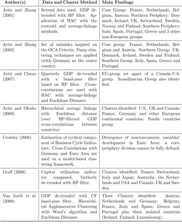
Table 1 includes some references on the application of clustering techniques in business
Table 1: Some Literature Review on Business Cycle Cluster Analysis
Author(s) Data and Cluster Method Main Findings Artis and Zhang
(2001)
Several data used: GDP de-trended with HP filter. Ap-plication of HAC with the centroid and average-linkage methods.
Core Group: France, Netherlands, Bel-gium, Austria; Northern Periphery: Den-mark, Ireland, UK, Switzerland, Sweden, Norway and Finland; Southern Periphery: Italy, Spain, Portugal, Greece and 2 other non-European groups.
Artis and Zhang (2002)
Set of variables inspired on the OCA Criteria. Fuzzy clus-tering techniques are applied (with Germany as the center country.
Core group: France, Netherlands, Bel-gium and Austria. Northern Group: UK, Denmark, Ireland, Sweden and Finland. Southern Group: Italy, Spain, Greece and Portugal.
Artis and Claeys (2007)
Quarterly GDP de-trended with a band-pass filter based on HP filter. Cross-correlations are used with HAC with average-linkage and Euclidean Distance.
EU-group set apart of a Canada-U.S. group. Scandinavian Group also identi-fied.
Artis and Okubo (2009)
Hierarchical average linkage with Euclidean distance (over HP-filtered GDP cross-correlations between countries)
Clusters identified: U.S., UK and Canada; France, Germany and other European continental countries; Nordic countries group.
Crowley (2008) Estimation of cyclical compo-nent of Business Cycle Indica-tors. Cross-Correlations with Germany and Euro Area are used on a model-based clus-tering framework.
Divergence of macroeconomic variables’ development in Euro Area; a core-periphery division cannot be fully defined.
Graff (2006) Capital utilization indica-tor composed, furtherly de-trended with HP filter.
Clusters identified: France, Switzerland, Italy and Japan; Australia, the Nether-lands and USA and Canada, UK and Swe-den.
Van Aarle et al. (2008)
GDP de-trended with CF band-pass filter. Hierarchi-cal Agglomerative Clustering with Ward’s algorithm and Euclidean Distance.
Three Clusters identified: Austria, Netherlands and Germany; Belgium, France, Italy and Spain; Greece and Portugal plus three isolated countries (Ireland, Finland, Luxembourg).
3
Methodology
This thesis investigates how European Business Cycles can be grouped into country-aggregate clusters, assessing its level of synchronicity, interdependence and response to
economic permanent shocks. Through the emprical analysis made in the present work, we have chosen a specific econometric and statistical framework, which is based in the following
features: Hierarchical Agglomerative Clustering (HAC), detection of Turning Points, met-rics for Business Cycle Synchronicity, stationarity analysis, Vector Autoregressive Model
(VAR), Granger-causality, Impulse Response Functions (IRF) and Forecast Error Variance Decomposition (FEVD).
3.1
Hierarchical Agglomerative Clustering
Having as a goal the identification of synchronous and identical groups of countries we
have pursuit a cluster analysis based on the Hierarchical Agglomerative Clustering (HAC) approach. The approach can be briefly described as follows: at first, each individual
country belongs to its own cluster; then, the algorithm groups the different countries in pairs that are the "most similar" (i.e. that have the smallest dissimilarity level); the process
is repeated iteratively until all countries in the sample belong to a unique cluster. Given our aims, we can say that the algorithm combines pairs of "most-synchronous" countries.
Albeit the variety of algorithms applied and explored in the literature, we chose to use the Ward’s algorithm introduced by Ward (1963) and the Euclidean distance as the metric
distance (dissimilarity measure). As it maximizes the homogeneity within the clusters, the Ward’s algorithm is considered a suitable tool for BC synchronization research (Van Aarle
et al., 2008).15.
The Ward’s algorithm calculates the distance for each pair of countries’ cyclical
com-15Other approaches to the Ward’s algorithm in Business Cycle research include Graff (2006),
Van Aarle et al. (2008) and Ductor and Leiva-Leon (2015). For robustness check, we have also tested the group-average and centroid algorithms following Artis and Zhang (2001). These methods were unable of grouping all countries into distinct clusters at some stage, and therefore were discarded due to the purpose of the present research.
ponents yi and yj based on the root of the quadratic linear Euclidean distance: d(yi, yj) = s X i (yi− yj)2 , yi 6= yj (1)
then the Ward’s algorithm proceeds to calculate the clusters on the basis of the min-imum increase in d(yi, yj). After merging two clusters into another, the algorithm then
calculates the distance between two other clusters as the increase in the error sum of the squares (ESS), i.e., the sum of squares of the deviations from the mean value, expressed
as ESS(X) = Nx X i=1 |xi − 1 Nx Nx X j=1 xj| 2 (2)
where X is a set of Nx values, xi represents the observation i from the set X, and xj
represents all the observations included in X used for the calculation of the mean value. The linkage function that expresses the distance between two clusters X and Y is
d(X, Y ) = ESS(XY ) − [ESS(X) + ESS(Y )] (3)
where XY stands for the new cluster formed by the merge of the cluster X and the cluster Y 16.
A variable (or in our case, a country deviation cycle) belongs to its own initial cluster at the last stage whenever it displays such a high level of dissimilarity to is counterparts
that the algorithm could not assign it to a specific group.
3.2
Turning Points Dating and Business Cycle metrics
The choice for the application of a filtering methodology (as described in section 4) to
estimate a deviation cycle has further implications on the dating of turning points in the series (Artis et al., 2004a). For dating the turning points we consider the Bry-Boschan
Quarterly (BBQ) algorithm developed by Harding and Pagan (2002), a modified version of the Bry-Boschan (BB) algorithm from Bry and Boschan (1971). Although initially
designed to be applied on classical business cycles (on series in levels or in growth rates),
16The Ward’s algorithm is applied with a MATLAB routine. The codes and execution steps
there is no impediment on its extension to de-trended series 17.
The BBQ algorithm defines peaks and troughs in the data as the local minima and
maxima. Considering zt as the cyclical component at time t a peak is defined as:
zt−2− zt < 0, zt−1− zt< 0; zt+1− zt< 0, zt+2− zt < 0 (4)
and a trough is defined as:
zt−2− zt > 0, zt−1− zt> 0; zt+1− zt> 0, zt+2− zt > 0 (5)
The BBQ considers a window over which local minima (trough) and maxima (peak) are calculated as being two quarters. The minimum phase length is set on two quarters and the
minimum full cycle length on five quarters in order to avoid spurious turning points. The BBQ algorithms also requires that phases alternate (a peak is always followed by a trough
and vice-versa)18. The STATA outcome from the BBQ algorithm is -1 for a trough, 1 for a peak and 0 otherwise.
After the turning point dating, we pursuit stylized measures to assess dis(similarities) between the clusters business cycles on frequency, duration, amplitude and slope. The
outcome of the STATA BBQ algorithm is substituted manually into a binary variable St
that assumes the value 1 whenever there is an expansion (i.e. between a -1 and a 1 ) and
0 whenever there is a contraction (i.e. between a 1 and a -1 ). We measure the average duration of a contraction between a peak and a trough as
DP T = PT t=1St PT −1 t=1(1 − St+1)St (6)
and the average duration of an expansion between a trough and a peak as
DT P = PT −1 t=1(1 − St) PT −1 t=1(1 − St)St+1 (7)
The numerators in (16) and (17) measure respectively the time spent in contractions
and expansions, and the denominators measure respectively the number of peaks and
17Examples of the BBQ application for growth cycles can be seen in Altissimo et al. (2001),
Zarnowitz and Ozyildirim (2006), Massman and Mitchel (2004) and an adaption in Artis et. al (2004b), among others
18We apply the BBQ algorithm on STATA with the code sbbq developed by Philipe Bracke
troughs. The amplitude of a phase Ai is the total growth between a peak (trough) and a
trough(peak), expressed as
Ai = zi(t+d)− zit (8)
where d is the total duration of a phase, zt the value for the growth cycle at a
peak(trough) and zt+d the value for the growth cycle on the succeeding trough(peak).
The average amplitude of an expansion phase is given by
AT P = PT t=1Ai(1 − St) PT −1 t=1(1 − St)St+1 (9)
and the average amplitude of a contraction phase by
AP T = PT t=1AiSt PT −1 t=1(1 − St+1)St (10)
Following Harding and Pagan (2002), we may consider Ai and Di = d as being the
height and base of a triangle, respectively. The area of such triangle provides the welfare
(or cumulative) loss(gain) of output in a recession(expansion), expressed as
CT i =
AiDi
2 (11)
Further we can consider an index of excess cumulated movements measure Ei given by
Ei = (CT i− Ci) Ci (12) with Ci = Ai 2 + d−1 X s=1 (yt+s− yt), s = 1, ..., d (13)
Ci represents the actual output cumulative movements, as CT i is the triangular
approx-imation for such. The excess cumulated movements Ei are calculated as the phase does
not evolve linearly between two extreme points.
We also consider a measure for the deviation cycle steepness for both expansionary and
contraction phases which represents the slope of the triangle. The steepness of phase i is given by:
Steepnessi =
Ai
Di
(14)
In order to measure synchronicity between the estimated deviation cycles, we calculate the Index of Concordance, the Pearson correlations and the Spearman’s rank correlations.
The Index of Concordance, introduced by Harding and Pagan (2002a), calculates the percentage of phases on which two series are synchronized, express as 19:
cxy = T−1 T
X
t=1
[Sx,tSy,t+ (1 − Sx,t)(1 − Sy,t)] (15)
where Si,t is the business cycle phase of the country i at time t (the same applies for
Sj,t) and T is the number of quarters considered in the sample. Si,t and Sj,t assume the
value of 1 whenever there is an expansion (growth is above trend) and 0 whenever there is a contraction (growth is bellow trend). As censoring rules were applied for the detection
of turning points, the distributional properties of cij are unknown. Therefore, the Index
of Concordance may be transformed into an empirical correlation between Si,t and Sj,t as
follows:
cxy = 1 + 2ρsσSxσSy+ 2µSxµSy− µSx− µSy (16)
where µsi and σsi, with i = x, y, represent respectively the mean and standard deviation
of Si,t. Further on, there is a linear relationship between cxy and ρS expressed as:
Sy,t σSy = η + ρS Sx,t σSx + ut (17)
where η is a constant and ut the error term. Equation (17) is estimated through OLS
with robust-standard errors to ensure that the estimator is consistent, since ut includes
serial correlation from Syt under the null hypothesis ρs = 0. This metric may be used
whenever pair is considered.
The Spearman’s rank correlation (1904) measures the strength and direction of the
monotonic relationship between two variables. It is calculated as the same as Pearson’s correlation but on the ranks and average ranks as follows:
r = 1 − 6 P
di2
T3− T (18)
on which di is the difference of ranks from the two variables for each observation, and
T the total number of observations.
19The Index of Concordance is also used in several works, for instance McDermott and Scott
(2000), Harding and Pagan (2002), Krolzig and Toro (2005) and Harding and Pagan (2006), among others.
3.3
Econometric Framework
The existence of stationarity on a time-series ensures the robustness of the statistical inference, avoiding spurious regressions. In fact, the to-be-executed econometric framework
based on the VAR model requires that all variables are stationary. The unit root test indicates if the time-series verify a time-invariant mean, variance and autocovariance, i.e.
if they are a stationary process.
The Augmented Dickey-Fuller (ADF) test is an extension of the Dickey-Fuller tests and
assume that residuals are serially correlated (Dickey and Fuller, 1979). The ADF test has the null hypothesis of the presence of a unit root, against the alternative of a stationary
process. Assuming Dtas a vector of deterministic terms, p the lagged difference terms and
∆yt−j an approach to an ARMA structure, the ADF test can be formulated as follows:
yt= β0Dt+ ϕyt−1+ p
X
j=1
ψ∆yt−j+ εt (19)
where the coefficient ϕ is the parameter of interest and included in a test statistic DF = ˆϕ/SE( ˆϕ), analyzed after the critical values of the DF t-distribution.
Amid the identification of the country-clusters on the first-stage, the VAR methodol-ogy is applied to both validate the component countries within and Cluster, and to assess
further on the economic impacts from the structural analysis. The VAR methodology, introduced by Sims (1980), consists on a n-equation, n-variable linear model in which
each variable is explained by its own lagged values and the past values of the remaining n-1 variables. Considering its reduced form, each variable is assigned with a linear func-tion estimated by OLS (Ordinary Least Squares) or Maximum Likelihood, on a dynamic simultaneous-equation economic model. A VAR of lag length equal to p - a VAR(p) - is a
process that evolves according to:
yt= Φ0+ Φ1yt−1+ Φ2yt−2+ ... + Φpyt−P + εt, t = 1, ..., T (20)
where yt is a n by 1 vector stochastic process, Φ0 is a k by 1 vector of intercept
parameters and Φj, j = 1, ..., p is a k by k parameter matrix. The white noise process is
denoted by εt. Moreover E[εt] = 0 and E[εtε0t−s] =
P
= 0, where P
time-invariant covariance matrix 20.
To determine the optimum lag length of each country-cluster VAR we proceed to use
the Akaike Information Criterion (AIC) through the minimization of the estimated number of lags j on the following equation:
min log(SSRj/T ) + (j + 1)C(T )/T (21)
Where SSRj is the Sum of Squared Residuals for the autoregression of j lags and j + 1
denotes the inclusion of the intercept term.
We also test the presence of autocorrelation of disturbances after computing the VARs with a Lagrange Multiplier test (LM Test). The LM test statistic is defined as:
LMs= (T − d − 0.5)ln
|cP|
|gPs|
(22)
where T is the total number of observations, d is the number of coefficients estimated,
c P
is the maximum likelihood estimate of P
and gPs the maximum likelihood estimate
for the variance-covariance matrix P
in the augmented VAR. The null hypothesis of the LM test is the non-existence of autocorrelation at an ex-ante defined lag order, and its
asymptotic distribution is a χ2
K2.
Amid the VAR specification, we initially verify its stability in order to proceed to
structural inference analysis, as covariance stationarity is not a sufficient condition to do so. A VAR is said to be stable if it can be re-written as a vector moving average (VMA),
which means that its respective polynomials are invertible. As such, IRF and FEVD results are keen to be interpreted. In this process, a matrix of eigenvalues A is computed, on which
the stability is confirmed whenever the modulus of each eigenvalue in A is strictly less than 1 (Lutkepohl, 2005 and Hamilton, 1994).
On the next step we pursuit a Granger-causality analysis, introduced by Granger (1969). Assuming a VAR(p) as in (20) it is said that yj,t does not Granger cause yi,t if all the
20More detailed information on VAR theory can be read in
Hamil-ton, J. D. (1994) chapter 11 or at chapter 5 of Sheppard, available at https://www.kevinsheppard.com/images/5/56/Chapter5.pdf.. Further equations and method-ologies were retrieved from the latter source.
coefficients of coefficient values of the latter on the first’s equation are zero. The Likelihood Ratio Test for Granger-causality is
(T − (pk2)).(ln|dX
r
| − ln|dX|) ∼Aχ2
P (23)
where P
r represents the estimated residual covariance matrix for the null hypothesis
of no Granger-causality and P
u is the estimated covariance of VAR(p).
Next we compute the IRF as the second approach of analysis. An IRF is a function of derivative/change of yi (an element of y) with respect to a shock in εj (an element of e) for
any j and i. Given that yt is covariance-stationary, the stable VAR(p) can be re-written
as a VMA process such
yt= µ + εt+ Ξεt−1+ Ξεt−2... = µ +
∞
X
i=0
Ξiεt−i (24)
where µ is a k x 1 time-invariant mean of yt and Ξi represent the IRFs. Ceteris paribus,
a one-unit standard-deviation increase in the kth element of εt−i on the jth element of yt
after i periods is given by the j, k element of Ξi. Given the contemporaneous correlation
between the terms ε, a matrix P is calculated to orthogonalize εtwhere P is the Cholesky
decomposition of P
for the Orthogonal IRFs (such that P
= P PT), which is dependent on the variables’ order in the VAR.
The third instrument we rely on for the structural analysis is the FEVD. It measures the part of the error of the variable’s j forecast variance after h periods that is due to the
orthogonalized innovations in the kth variable. The FEVD depends on the choice of the matrix P. Re-writing the forecast errors as orthogonalized, the FEVD will measure the
4
Data and Business Cycle Estimation
In order to estimate the national business cycles we consider quarterly GDP retrieved from the OECD Quarterly National Accounts. The series are volume estimates in chain,
measured in US Dollars and constant prices with fixed PPPs (with OECD reference year equal to 2010). The data is already seasonally adjusted and expressed at annual levels 21.
The choice of the VPVOBARSA database was mainly due to the harmonization of each national series in the same currency (US Dollar), which allows the estimation of further
country-cluster aggregates without the need of using exchange-rates for such a long period. As the data is presented in volumes, we transform it into logarithms and proceed to
calculate the growth rates of each quarter compared to the same quarter of the previous year. The dataset comprehends a time span between the first quarter of 1960 (1960Q1)
and the first quarter of 2016 (2016Q1). Given our research purpose, we only consider European countries that were part of the European Exchange Rate Mechanism (ERM) at
some point of time, which accounts for the majority of Western, Northern and Southern European countries. Norway is not considered as it was never part of the ERM system nor
belongs to the Euro Area and European Union. The countries included are:
Austria (AT)
• • Belgium (BEL) • Denmark (DEN)
Finland (FIN)
• • France (FRA) • Germany (GER)
Greece (GRE)
• • Ireland (IRL) • Italy (ITA)
the Netherlands (NTH)
• • Portugal (POR) • Spain (SPA)
Sweden (SWE)
• • United Kingdom (UK)
In the words of Harding and Pagan (2002), to depict a cycle one first needs to define it. Here we deal with the deviation (or growth) business cycle in the light of the work of Lucas
21The database measure code is VPVOBARSA, available at the OECD Quarterly National