Repositório ISCTE-IUL
Deposited in Repositório ISCTE-IUL:
2019-01-18
Deposited version:
Post-print
Peer-review status of attached file:
Peer-reviewed
Citation for published item:
Martins, L. F. (2018). Bootstrap tests for time varying cointegration. Econometric Reviews. 37 (5), 466-483
Further information on publisher's website:
10.1080/07474938.2015.1092830
Publisher's copyright statement:
This is the peer reviewed version of the following article: Martins, L. F. (2018). Bootstrap tests for time varying cointegration. Econometric Reviews. 37 (5), 466-483, which has been published in final form at https://dx.doi.org/10.1080/07474938.2015.1092830. This article may be used for non-commercial purposes in accordance with the Publisher's Terms and Conditions for self-archiving.
Use policy
Creative Commons CC BY 4.0
The full-text may be used and/or reproduced, and given to third parties in any format or medium, without prior permission or charge, for personal research or study, educational, or not-for-profit purposes provided that:
• a full bibliographic reference is made to the original source • a link is made to the metadata record in the Repository • the full-text is not changed in any way
The full-text must not be sold in any format or medium without the formal permission of the copyright holders. Serviços de Informação e Documentação, Instituto Universitário de Lisboa (ISCTE-IUL)
Bootstrap Tests for Time Varying Cointegration
Luis F. Martins
Department of Quantitative Methods, ISCTE-IUL, Portugal, and
Centre for International Macroeconomic Studies, University of Surrey, UK
May 27, 2015
Abstract
This paper proposes wild and the i.i.d. parametric bootstrap implementations of the time-varying cointegration test of Bierens and Martins (2010, Econometric Theory 26, 1453-1490). The bootstrap statistics and the original likelihood ratio test share the same …rst-order asymptotic null distribution. Monte Carlo results suggest that the bootstrap approximation to the …nite-sample distribution is very accurate, in particular for the wild bootstrap case. The tests are applied to study the purchasing power parity hypothesis for twelve OECD countries and we only …nd evidence of a constant long-term equilibrium for the U.S.-U.K. relationship.
Keywords: Time-Varying Cointegration, Bootstrap, Likelihood Ratio Test, Pur-chasing Power Parity Hypothesis.
J.E.L. Classi…cation: C12, C32.
Av. das Forças Armadas, 1649-026 Lisbon, Portugal. Telephone: +351 21 790 3439. E-mail: [email protected]. Comments from the editors and two referees, participants at the Conference in Honor of Herman Bierens and the 10th BMRC-DEMS Conference on Macro and Financial Eco-nomics/Econometrics and …nancial support under grant PTDC/EGE-ECO/122093/2010 from the Fun-dação para a Ciência e Tecnologia are gratefully acknowledged.
1
Introduction
Structural change is of key importance in economics and econometrics, especially for coin-tegration analysis, as it normally involves long term historical trends, which, consequently, are likely to display breaks in their equilibrium relationship. In a recent paper, Bierens and Martins (2010) proposed a vector error correction model in which the cointegration vec-tors change smoothly over time and, from that model, a likelihood ratio test for standard time-invariant cointegration. Despite the simplicity of the test, the asymptotic chi-square distribution appears to be a poor approximation to the relevant …nite-sample distribu-tion. In particular, the test falsely indicates the existence of time-varying cointegration too often.
To address this problem, we propose in this paper a bootstrap algorithm for obtain-ing critical values and show that this alternative approach does lead to test procedures that have, approximately, the correct size. As in many other estimation and inference contexts, in our case the bootstrap distribution is also an accurate approximation to the …nite-sample one under the null hypothesis of constant cointegration vectors, as initially presented by Johansen (1988, 1991 and 1995).
It has extensively been shown in the literature that bootstrap methods provide higher order asymptotic re…nements and, thus, better results in bias reduction, con…dence inter-val construction and hypothesis testing in …nite-samples, even in the cases where analytical results are known. See, for example, Jeong and Maddala (1993), Horowitz (2001), as well as Li and Maddala (1996) and Härdle, Horowitz and Kreiss (2001) surveys, the last two in the time series context. As an example in the structural breaks literature, Diebold and Chen (1996) demonstrate the bene…ts of bootstraping the ‘supremum’tests of Andrews (1993).
The likelihood ratio bootstrap tests we suggest follow very closely those already pro-posed in the literature for testing and determining the cointegration rank in VAR models. Swensen (2006) consider an i.i.d. bootstrap version of the pseudo LR trace test statistic whereas Cavaliere, Rahbek and Taylor (2010a) advocate the usage of the wild bootstrap instead as it provides better results under conditional heteroskedasticity when compared to the i.i.d. procedure. Moreover, Cavaliere, Rahbek and Taylor (2012) propose a bootstrap scheme that improves Swensen’s approach to create bootstraped data once the VECM is
estimated under the null hypothesis and not under both hypothesis as in Swensen (2006).1
The contents of the paper are as follows. In Section 2, we review the time-varying VECM and the original LR test for time-invariant cointegration and introduce the wild and i.i.d. parametric bootstrap versions of the pseudo LR test, showing their consistency because the three share the same chi-square asymptotic distribution. Section 3 sets out the designs of the Monte Carlo experiments and suggests that the bootstrap approximation to the …nite-sample distribution is very accurate, especially for the wild bootstrap. Finally, Section 4 discusses the purchasing power parity hypothesis in the context of time-varying cointegration and reports results from an application of the methodology to international prices and nominal exchange rates.
2
Bootstrap Time-Varying Cointegration Tests
2.1
The Time-Varying Cointegration Model
As in Bierens and Martins (2010), consider the time-varying VECM(p) with a drift,
4Yt= + 0 tYt 1+ p 1 X j=1 j4 Yt j+ "t; t = 1; :::; T; (1)
where Yt 2 Rk; "t2 Rk; ; ; and the j’s are …xed coe¢ cients, the t’s are time-varying
(TV) k r matrices of cointegrating vectors, and T is the number of observations. 2 The
initial values Yt; t = 0; 1; :::; p + 1; are assumed to be …xed. The LR test is de…ned
for the null hypothesis of standard time-invariant (TI) cointegration, t = for all t;
1In the context of cointegrated VAR models, see also the bootstrap approaches of Trenkler (2009) - i.i.d.
bootstrap where in a …rst stage the deterministic terms are estimated by a feasible GLS procedure - and Cavaliere, Rahbek and Taylor (2010b) - wild bootstrap under non-stationary volatility. van Giersbergen (1996), Harris and Judge (1998) and Mantalos and Shukur (2001) focus on the properties of the bootstrap by means of Monte Carlo simulations. For bootstrapping methods in standard unit root testing, see, for example, Park (2003) and Paparoditis and Politis (2003).
2In this Bierens and Martins (2010) baseline model, there is a drift in Y
twhich is denoted by : This
does not cover all the usual leading cases for the deterministic components within standard cointegration test frameworks. In particular, we do not consider the cases of the intercept being absorbed into the cointegration relation and the existence of a linear trend. Accounting for a trend is not straightforward in time-varying cointegration as pointed out by Bierens and Martins (2010).
against time-varying cointegration (TVC) in which the cointegrating relationship varies smoothly over time, maintaining the number of cointegration relations as equal to r < k: In this test setup, there must exist a …xed certain number of cointegration relations, r > 0: Time-varying cointegrating systems do not necessarily generate time-varying cointegration spaces. The conditions for the existence of time-invariant or time-varying cointegration spaces can be found at Martins and Gabriel (2013). Assuming that the function of discrete
time t is smooth (see Bierens and Martins (2010) for details), it can be written as
t= m(t=T ) =
m
X
i=0
i;TPi;T (t) (2)
for some …xed m < T 1;where the orthonormal Chebyshev time polynomials Pi;T (t)are
de…ned by P0;T (t) = 1; Pi;T (t) =
p
2 cos (i (t 0:5) =T ) ; t = 1; 2; :::; T; i = 1; 2; 3; :::; mand
i;T = T1
PT
t=1 tPi;T (t) are unknown k r matrices.
Similar to Johansen (1988, 1991 and 1995), model (1) can be speci…ed more conve-niently as
4Yt=
0
Yt 1(m)+ Xt+ "t; (3)
where 0 = 00; 01; :::; 0m is an r (m + 1)k matrix of full rank r, Yt 1(m) is de…ned by
Yt 1(m) = Y0 t 1; P1;T (t) Yt 10 ; P2;T (t) Yt 10 ; :::; Pm;T (t) Yt 10 0 and = ( ; 1; :::; p 1) and Xt = 1;4Y 0 t 1; :::;4Y 0 t p+1 0
:Under the null hypothesis, 0 = ( 0; 0r;k:m) ;where is the
standard k r matrix of TI cointegrating vectors, so that then 0Yt 1(m) = 0Yt 1(0)
0Y
t 1: Therefore, given m and r; the LR test takes the form
LRtvcm;T = T r X j=1 ln 1 b0;j 1 bm;j ! ; (4)
where 1 > bm;1 bm;2 ::: bm;r ::: bm;(m+1)k are the ordered solutions of the
generalized eigenvalue problem deth S11;T(m) S10;T(m)S00;T1 S01;T(m)i = 0 with
S00;T = 1 T T X t=1 4Yt4 Y 0 t 1 T T X t=1 4YtX 0 t ! 1 T T X t=1 XtX 0 t ! 1 1 T T X t=1 Xt4 Y 0 t ! ; (5) S11;T(m) = 1 T T X t=1 Yt 1(m)Yt 1(m)0 1 T T X t=1 Yt 1(m)Xt0 ! 1 T T X t=1 XtX 0 t ! 1 1 T T X t=1 XtY (m)0 t 1 ! ; (6)
S01;T(m) = 1 T T X t=1 4YtY (m)0 t 1 1 T T X t=1 4YtX 0 t ! 1 T T X t=1 XtX 0 t ! 1 1 T T X t=1 XtY (m)0 t 1 ! ;(7) S10;T(m) = S01;T(m) 0: (8)
The b0;j’s are similarly de…ned by imposing m = 0 (standard cointegration).
Assuming that the errors are i.i.d. Gaussian, i.e., "t i:i:d: Nk[0; ] ; Bierens and
Martins (2010) show that, given m 1and r 1; under the null hypothesis of standard
cointegration, LRtvcm;T is asymptotically 2mkr distributed. They also concluded that, for
small T and large m; the test su¤ers from size distortions and tends to overreject the correct null hypothesis of standard cointegration. Given this result, we propose in the
next Section two bootstrap versions of LRtvcm;T along the lines of Cavaliere, Rahbek and
Taylor (2010a, 2012) and Swensen (2006).
Following the seminal work by Johansen (1988, 1991, 1995), Bierens and Martins
(2010) take the normal distribution for "t and from that derive the exact likelihood
func-tion and LR statistic. Actually, imposing normality is not necessary for deriving the
asymptotic distribution of LRtvc
m;T under the null hypothesis. By simply assuming i.i.d.
errors, a straightforward but tedious exercise would be to show that the pseudo LRm;Ttvc
statistic is also asymptotically 2
mkr distributed when based on the pseudo Gaussian
like-lihood function.3
In terms of the bootstrap approach, we relax the original assumptions by taking those at Cavaliere, Rahbek and Taylor (2010a) under our context of standard cointegration:
Assumption 1.
(a) For m = 0; the usual conditions related to the characteristic roots and the
nonsin-gularity of matrix 0(I
k 1 ::: p 1) are taken to be true.
(b) The innovations f"tg form a martingale di¤erence sequence with respect to the
…ltration Ft; where Ft 1 Ft for t = :::; 1; 0; 1; 2; :::; satisfying (b1) the global
ho-moskedasticity condition 1 T T X t=1 E ("t"0tjFt 1) p ! > 0 (9)
3In this case, the exact likelihood function and the pseudo Gaussian likelihood function would coincide
and therefore the last piece of the proof of Bierens and Martins (2010)’ Theorem 1, where a Taylor expansion around the MLE of a particular function, would follow through.
and (b2) E k"tk4 K <1:
Remark. Here, f"tg is serially uncorrelated and possibly conditionally heteroskedastic.
Instead, Cavaliere, Rahbek and Taylor (2012) and Swensen (2006) assume i.i.d. innova-tions. See Cavaliere, Rahbek and Taylor (2010a) for more details about the underlying di¤erences and the functional central limit theorem and the law of large numbers that apply to martingale di¤erence sequences.
2.2
Bootstrap Tests
The parametric bootstrap versions of the TVC test statistic we consider are the wild boot-strap and the i.i.d. bootboot-strap. They both are implementations to TVC of the Cavaliere, Rahbek and Taylor (2010a, 2012) (wild and i.i.d.) and Swensen (2006) (i.i.d.) bootstrap procedures for testing the cointegration rank. Next, we de…ne the bootstrap procedures
using the unrestricted residuals (and b; b) as in Cavaliere, Rahbek and Taylor (2010a)
and Swensen (2006) and at the end of this Section we de…ne the alternative procedure
based upon the restricted residuals (andb; b) as in Cavaliere, Rahbek and Taylor (2012).
As in Cavaliere, Rahbek and Taylor (2010a), we construct the pseudo Gaussian like-lihood function and the pseudo LR test by assuming i.i.d. Gaussian errors. For the
unrestricted TVC model (3), m > 0; let b; b denote the pseudo maximum likelihood
(ML) estimate of ( ; ) and b"t; t = p + 1; :::; T; the pseudo ML residuals. Moreover, let
b; b denote the restricted pseudo ML estimates of ( ; ) under the null hypothesis of standard cointegration, m = 0: The bootstrap algorithms are described as follows:
Wild bootstrap test for TVC using the unrestricted residuals First, generate
B bootstrap pseudo-disturbances "b
t; t = p + 1; :::; T and b = 1; :::; B; from residuals b"t
according to "b
t =b"twtwhere fwtgTt=p+1is an independent N (0; 1) scalar sequence. Second,
construct the bootstrap sample 4Ytb
T
t=1 recursively from the equation
4Ytb =b + bb 0 Yt 1b + p 1 X j=1 bj4Yb t j+ " b t; t = 1; :::; T; (10)
with initial values Ytb = Yt; t = 1; :::; p: Third, using the bootstrap sample, 4Ytb
T t=1;
construct the bootstrap LR test statistic, LRb
m;T = T Pr j=1ln 1 bb0;j 1 bbm;j ; where the bb’s
denote the bootstrap versions of the ordered generalized eigenvalues b’s. Fourth, the bootstrap 95% percentile of the resulting distribution is used as the 5% critical value
for the bootstrap test procedure. In a similar manner, bootstrap p-values pb
m;T for the
test statistic LRtvc
m;T are computed as pbm;T = 1 Fm;Tb LRtvcm;T ; where, conditional on
the original data fYtg ; Fm;Tb ( ) denotes the cumulative distribution function of LRbm;T:
Because the bootstrap distribution Fb
m;T is a complicated function of fYtg, in practice, pbm;T
is obtained through the numerical approximation: peb
m;T = B1
PB
b=11 LR b
m;T > LRtvcm;T :
Fifth, for a signi…cance level ; reject the null hypothesis of standard cointegration if e
pb
m;T < :
As pointed out by Cavaliere, Rahbek and Taylor (2010a), an alternative could be
drawing from equation (10) but without the estimate of the deterministic part, b; and
setting initial values to zero, Yb
t = 0; t = 1; :::; p:See Cavaliere, Rahbek and Taylor (2010a,
2012), Swensen (2006) but also Cavaliere, Rahbek and Trenkler (2013) for a discussion on
why the rank statistic is invariant with respect to and recall that Bierens and Martins
(2010) showed that LRtvc
m;T has the same distribution whether or not there is an intercept
in the model.
Swensen’s i.i.d. bootstrap test for TVC Same as the wild bootstrap approach
except that the bootstrap pseudo-disturbances "b
t; t = p+1; :::; T;are drawn randomly with
replacement from the residualsb"t: Following the same argument as in Cavaliere, Rahbek
and Taylor (2010a), obtain instead the centered residuals nb"t T1p
PT
i=p+1b"i
oT
t=p+1 if
drawing from equation (10) without the intercept term.
The number of bootstrap pseudo-samples B must be "large enough" since peb
m;T
con-verges to pb
m;T as B increases. In their numerical experiments, Cavaliere, Rahbek and
Taylor (2010a, 2012) set B = 399 and Swensen (2006) considers B = 5000: In the next Theorem we show that the …rst-order asymptotic distributions of the bootrastrap TVC test statistics and the Bierens and Martins (2010) original TVC test statistic are the same. Moreover, in the next Section, we provide, by means of simulations, evidence that the bootstrap approximation to the …nite sample distribution seems to be much more accu-rate, as opposite to the asymptotic approximation. Hence, we consider the wild and i.i.d. bootstrap versions of the TVC test statistic as valid ones to test for standard cointegration
and recommend using their critical values to ensure correct 5% type-I errors, say.
The proof of Theorem 1 is presented in a similar way as in Cavaliere, Rahbek and Taylor (2010a, 2012) and Swensen (2006). Note that, under the null hypothesis, our model is the same as in Cavaliere, Rahbek and Taylor (2010a, 2012) and Swensen (2006) and the assumptions as in Cavaliere, Rahbek and Taylor (2010a). We also consider the wild and the i.i.d. bootstraps but the di¤erence is that, in our context, we test against TVC and …x r.
Theorem 1. Let LRwb
m;T and LRsbm;T denote the LRbm;T bootstrap test statistics for the
wild and i.i.d. cases, respectively. Given m 1 and r 1; under the null hypothesis of
standard cointegration and Assumption 1, the bootstrap LR statistics LRwb
m;T and LRm;Tsb
de…ned above are asymptotically 2
mkr distributed, as T ! 1:
Proof : For sake of simplicity, and as in Cavaliere, Rahbek and Taylor (2010a), we
take the no-drift case, = 0; for which Bierens and Martins (2010) showed that LRtvc
m;T is
also asymptotically 2
mkr distributed. To avoid confusion with the "wb=sb" notation, we
denote any of the two bootstrap probabilities by P and the expectation under P by E
and we do, similarly, with the bootstrap quantities Yb
t; "bt; Rbt;T; :::
Under standard cointegration, we have from Cavaliere, Rahbek and Taylor (2010a) that (i) Ytb = bC t X i=p+1 "bi +pT Rbt;T; t = p + 1; :::; T; (11)
where for all > 0; P max
p+1 t T R b t;T >
p
! 0 as T ! 1; j j is the usual Euclidean
distance and bC = b? b0?bb?
1
b0?; (ii) 4Ytb =
Pt 1
i=0bi"bt i; where bi are exponentially
decreasing coe¢ cients, (iii) E "b
t"b0t = bb p ! as T ! 1; and (iv) 1 p T b T c X i=p+1 "bi ! W ( ) ;w (12)
where W (u) ; u 2 [0; 1] is a k dimensional Wiener process with covariance matrix :
Contrary to Cavaliere, Rahbek and Taylor (2010a, 2012) and Swensen (2006), b and b"t
are obtained from the TVC model (3) and, as a result, our bootstrap samples Ytb; "bi; Rbt;T
are di¤erent from theirs. The formulas for Rb
t;T are in Cavaliere, Rahbek and Taylor
With the following Lemmas, we show that the TVC test statistic applied to the
boot-straped sample, LRm;Tb ; is also asymptotically 2
mkr distributed, as T ! 1: The
Lem-mas are as those at Bierens and Martins (2010) involving the matrices Sij;T(m); i; j = 0; 1;
but with bootstrapped data Yt 1b;(m) = Yb0
t 1; P1;T (t) Yt 1b0 ; P2;T (t) Yt 1b0 ; :::; Pm;T (t) Yt 1b0 0 and Xb t = 4Yb 0 t 1; :::;4Yb 0 t p+1 0
and invoking the functional central limit theorem and the law of large numbers that apply to martingale di¤erence sequences instead (Brown, 1971, and Hannan and Heyde, 1972), and where it is shown that the original limiting results still hold. Lemma 1. Let l = 1; :::; p 1: As T ! 1; 1 T T X t=1 "btYt 1b;(m)0!d Z 1 0 (dW (u)) fWm(u)0(C0 Im+1) (13) 1 T T X t=1 4Yt lb Y b;(m)0 t 1 d ! C Z 1 0 (dW (u)) fWm(u)0(C0 Im+1) + Mlb (14) 1 T2 T X t=1 Yt 1b;(m)Yt 1b;(m)0 ! (Cd Im+1) Z 1 0 f Wm(u) fWm(u)0du (C0 Im+1) ; (15)
where W (u) is a k-variate standard Wiener process, f
Wm(u) = W0(u) ;
p
2 cos( u)W0(u) ; :::;p2 cos(m u)W0(u) 0;
the Mb
l’s are k k(m + 1) non-random matrices and C = ?( 0? ?)
1 0 ?.
Proof : Let u 2 [0; 1] ; …x j; h = 1; :::; m and let l = 1; :::; p 1: For the …rst result,
note that 1 T T X t=1 Pj;T(t) "btYb 0 t 1 = p 21 T T X t=1 cos (j (t 0:5) =T ) "bt t 1 X i=p+1 "bi0Cb0 +p21 T T X t=1 cos (j (t 0:5) =T ) "btpT Rb0t 1;T:
From Bierens (1994), Lemma 9.6.3., page 200, 1 T T X t=1 cos (j (t 0:5) =T ) "bt t 1 X i=p+1 "bi0 = cos (j (1 0:5=T )) 1 T T X t=1 "bt t 1 X i=p+1 "bi0+ j Z 1 0 sin (j (u 0:5=T )) 0 @1 T buT c X t=1 "bt t 1 X i=p+1 "bi0 1 A du
and 1 T T X t=1 cos (j (t 0:5) =T ) "btpT Rb0t 1;T = cos (j (1 0:5=T )) 1 T T X t=1 "btpT Rb0t 1;T + j Z 1 0 sin (j (u 0:5=T )) 0 @1 T buT cX t=1 "btpT Rb0t 1;T 1 A du;
where the last term vanishes because for all > 0;
P 0 @ max p+1 t T 1 p T buT cX t=1 "btRb0t 1;T > 1 A < P 0 @ max p+1 t T 0 @ p1 T buT cX t=1 "bt Rb0t 1;T 1 A > 1 A < p1 T buT c X t=1 "bt :P max p+1 t T R b0 t 1;T > p ! 0 as T ! 1:
From (12) and the continuous mapping theorem (CMT), the …rst term converges in dis-tribution to cos (j ) Z 1 0 dW (u) W (u)0+ j Z 1 0 sin (j u) Z u 0 dW (y) W (y)0 du = Z 1 0
(dW (u)) cos (j u) W (u)0;
via integration by parts (see Bierens and Martins (2010)). Then, 1 T T X t=1 Pj;T(t) "btY b0 t 1 d ! Z 1 0
(dW (u))p2 cos (j u) W (u)0C0 as T ! 1
due to convergence in probability of bC (see Bierens and Martins (2010) for the limiting
properties of the pseudo MLE bC and the Proof of Lemma S2 in the Supplement to
Swensen (2006), available at Econometrica’s website, for why the CMT still holds under
P )and the result follows.
For the second result, 1 T T X t=1 Pj;T (t)4Yt lb Y b0 t 1 = 1 T T X t=1 Pj;T (t)4Yt lb Y b0 t 1 Y b0 t 1 l + 1 T T X t=1 Pj;T(t)4Yt lb Y b0 t 1 l
where 1 T T X t=1 Pj;T(t)4Yt lb Y b0 t 1 l = p2 cos (j (1 0:5=T )) 1 T T X t=1 4Yt lb Y b0 t 1 l +p2j Z 1 0 sin (j (u 0:5=T )) 0 @1 T buT cX t=1 4Yt lb Y b0 t 1 l 1 A du: Cavaliere, Rahbek and Taylor (2010a) show that, under standard cointegration,
1 T buT cX t=1 4Yt lb Y b0 t 1 l d ! C Z u 0 dW (y) W (y)0 C0+ uM0b; where Mb
0 is the nonrandom k k matrix that de…nes the limiting variance term
E pT Rb t;T p T Rb0 t;T : Hence, 1 T PT t=1cos (j ((t 0:5) =T ))4Y b t lYb 0 t 1 l converges in distribution to cos (j ) C Z 1 0 dW (u) W (u)0 C0+ M0b +j Z 1 0 sin (j u) C Z u 0 dW (y) W (y)0 C0+ uM0b du = C Z 1 0
(dW (u)) cos (j u) W (u)0 C0;
(see Bierens and Martins (2010) for the equality). On the other hand, 1 T T X t=1 Pj;T (t)4Yt lb Y b0 t 1 Y b0 t 1 l = 1 T T X t=1 Pj;T (t) bC"bt l"b0t lCb0+ 1 T T X t=1 Pj;T(t) p T Rbt 1 l;T pT Rb0t 1 l;T + op(1) p ! Mj;lb ; say. Then, 1 T T X t=1 Pj;T(t)4Yt lb Y b0 t 1 d ! C Z 1 0
(dW (u))p2 cos (j u) W (u)0 C0 + Mj;lb
For the last one, again, by Bierens (1994), Lemma 9.6.3., 1 T2 T X t=1 Ph;T(t) Pj;T(t) Yt 1b Y b0 t 1 = 2 cos (h (1 0:5=T )) cos (j (1 0:5=T )) 1 T2 T X t=1 Yt 1b Yt 1b0 2 Z 1 0 d ducos (h (u 0:5=T )) cos (j (u 0:5=T )) 0 @ 1 T2 buT cX t=1 Yt 1b Yt 1b0 1 A du: From Cavaliere, Rahbek and Taylor (2010a),
1 T2 buT cX t=1 Yt 1b Yt 1b0 ! Cd Z u 0 W (y) W (y)0dy C0;
and the result holds given that 1 T2 T X t=1 Ph;T (t) Pj;T (t) Yt 1b Yb 0 t 1 d ! 2C Z 1 0
cos (h u) W (u) cos (j u) W (u)0du C0:
(see Bierens and Martins (2010) for the integration by parts).
Lemma 2. Let ? and ? be the orthogonal complements of and ;respectively. The
following quantities have the same limiting laws as in Bierens and Martins (2010): ( ?0 ?) 1=2 0?S01;Tb;(m)( 0? Im+1) ; (16) p T ( 0? ?) 1=2 0?S01;Tb;(m)( Im+1) ; (17) 0 1 1 0 1Sb;(m) 01;T ( 0? Im+1) ; (18) 0 1 1 0 1Sb;(m) 01;T ( Im+1) ; (19) 0 I m+1; T 1=2 0? Im+1 S b;(m) 10;T S b; 1 00;TS b;(m) 01;T Im+1; T 1=2 0? Im+1 and(20) T 1=2 0? Im+1; 0 Im+1 S11;Tb;(m) T 1=2 0? Im+1; Im+1 : (21)
Proof : It follows from Lemma 1, given the de…nition of Sij;Tb;(m); i; j = 1; 2 (see above)
and the sequence of arguments in Bierens and Martins (2010). Notice that these results are related to Lemma A6 at Cavaliere, Rahbek and Taylor (2010a) and Lemma S2 at Swensen (2006) (for i.i.d. errors) where in their case m = 0: In our test, m being greater than zero implies deriving the limiting laws of processes that involve the Chebishev polynomials. That is provided by the previous Lemma 1.
Lemma 3. Under the null hypothesis of standard cointegration and Assumption 1 and if > 0;
P S00;Tb XX > ! 0 (22)
P S01;Tb;(m)b X > ! 0 (23)
P b0S11;Tb;(m)b > ! 0 (24) in probability, where k k is the Euclidean norm and
XX = p lim T !1 1 T T X t=1 XtX 0 t; X = p lim T !1 1 T T X t=1 XtYt 10 = p lim T !1 1 T T X t=1 0 Yt 1Yt 10 :
Proof : The results were shown by Cavaliere, Rahbek and Taylor (2010a) (Lemma A7) and Swensen (2006) (Lemma S1, for i.i.d.) for the case of m = 0: As in Lemma 2, the results of this Lemma for any m > 0 follow from Lemma 1.
Lemma 4. Under the null hypothesis of standard cointegration and Assumption 1, the r
largest ordered solutions bbm;1 b
b
m;2 ::: b b
m;r of the generalized eigenvalue problem
deth S11;Tb;(m) S10;Tb;(m)S00;T1;bS01;Tb;(m)i = 0 (25)
converge in probability to constants 1 > 1 ::: r > 0; which do not depend on m.
Thus, these probability limits are the same as in the standard TI cointegration case:
det 0 1 1+ 1 = 0; (26) where = 0 X 1 XX X : Moreover, T bbm;r+1; bbm;r+2; :::; bm;kb 0 d! m;1; :::; m;k r 0; (27)
where m;1 m;2 :::: m;k r are the k r largest solutions of the generalized
eigenvalue problem det 2 4 0 @ R1 0 Wfk r;m(u)fWk r;m0 (u)du O(k r)(m+1);r:m Or:m;(k r)(m+1) Ir:m 1 A (28) 0 @ R1 0 Wfk r;m(u)dWk r(u)0 V 1 A Z 1 0 (dWk r(u)) fWk r;m(u)0; V0 3 5 = 0;
where Wk r(u) is a k r variate standard Wiener process,
f
Wk r;m(u) = ( 0? ?) 1=2 0
?C0 Im+1 Wfm(u);
and with V an r:m (k r) random matrix with i.i.d. N [0; 1] elements.
Proof : It follows from applying the previous results to the correspondent Lemmas at Bierens and Martins (2010) (A7, A8 and A9). Just as in Bierens and Martins (2010), we need to de…ne ?;T = 0 @ ? Im+1; 0 @ Opk;m:r T 1=2 Im 1 A 1 A to prevent T 1 0 ?;TS b;(m)
11;T ?;T from converging to a singular matrix (see Andersson et al.,
1983). See Theorems 3 and 4 at Cavaliere, Rahbek and Taylor (2010a) and Proposition 1 at Swensen (2006) (i.i.d.) for the case of m = 0:
Proof of Theorem 1. Following the same route as in Bierens and Martins (2010),
the 2
mkr distribution of the bootstrap TVC test statistic follows from a combination of
gaussian and 2 processes, as shown by Johansen (1995), once we apply the Taylor
expan-sion of Johansen (1988) around the pseudo MLE to the pseudo LR statistic. Recall that the exact ML function (Bierens and Martins (2010)) is the same as the pseudo ML func-tion once we assume Gaussian disturbances. To that end, and given the previous Lemmas,
we state that the pseudo ML estimator of with a bootstrapped sample, bb = bb1; :::; bbr ;
where bbi; i = 1; :::; r; are the eigenvectors associated with the r largest eigenvalues bbm;i;
S10;Tb;(m)S00;T1;bS01;Tb;(m)bib = bbm;iS11;Tb;(m)bbi; i = 1; ::; r; (29) has the same limiting distribution as the one in Bierens and Martins (2010). More
specif-ically, for the normalization eb = bb 0bb
1
0
with a partition eb = eb00; eb0m ; where
ebm is a k:m r matrix, and under the null hypothesis of standard cointegration,
T eb0 ! (d ?; Ok;k:m) Z 1 0 f Wk r;m(u)fWk r;m0 (u)du 1 (30) Z 1 0 f Wk r;m(u) dW (u)0 0 1 1=2 p T ebm !d 1=2 Im V 0 1 1=2 ; (31)
where W is an r-variate standard Wiener process, V is a k:m r matrix with
can be shown by generalizing Lemma A6 of Cavaliere, Rahbek and Taylor (2010a) and Lemma S2 of Swensen (2006) (Supplementary Material) (i.i.d.) to the case of m > 0: That can be done given our Lemma 1 that involves the Chebishev polynomials. See also page 9 of the Supplementary Material to Swensen (2006)’s paper for why the continuous mapping theorem still holds under P :
Bootstrap test for TVC using the restricted residuals In the context of the
LR cointegration rank test and associated sequential rank determination procedure of Johansen (1995), Cavaliere, Rahbek and Taylor (2012) show that important gains can
be achieved once the residuals (and b; b) are obtained from the cointegration model
under the null hypothesis. In particular, the bootstrap sequential rank determination procedure consistently determines the cointegration rank, in the sense that the probability of choosing a rank smaller than the true one will converge to zero.
As mentioned before, in our test for time varying cointegration, the cointegration rank, r, is …xed and assumed to be known and therefore the "sequential rank determination procedure" is not relevant in our framework. Still, we see no reason why using restricted residuals shouldn’t work as well for bootstrap TVC testing and, thus, suggest it as an alternative to the unrestricted procedure de…ned above.
Let all estimated quantities be exclusively obtained from the standard time invariant
cointegration model, m = 0 : b; b; b; b and b"t; t = 1; :::; T: Following Cavaliere, Rahbek
and Taylor (2012), this alternative Wild and i.i.d. bootstrap procedure is the same as the
one above but (i) the bootstrap pseudo-disturbances "b
t are obtained from the restricted
residualsb"t; and (ii) the bootstrap sample 4Ytb
T
t=1 is constructed from the same
equa-tion with all estimated coe¢ cients obtained under the null hypothesis. According to the Monte Carlo results shown in the next Section, this bootstrap procedure is surely also asymptotically correctly sized but, apparently, not applicable to some particular mod-els. We suspect that the usual bootstrap procedures using the restricted residuals are not suitable for models with r > 1 under conditionally heteroskedastic errors and, thus, alternative methods need to be proposed in the literature.
3
Monte Carlo Study
In this Section we illustrate the merits of the Bootstrap TVC tests by assessing their …nite-sample size performance through numerical simulations. We consider three cointegration models that follow closely the literature and combine distinct values for the number of cointegrating vectors, the number of variables in the system and the VAR lag order.
3.1
The Designs
The data generating processes (DGP’s) correspond to the standard cointegrated VAR’s (m = 0) presented by Bierens and Martins (2010) (denote it by BM), Johansen (2002) and Swensen (2006) (JS) and Engle and Yoo (1987) (EY). In the BM model there is a single cointegrating relationship driving a bivariate system and where p = 2; The JS model is instead of dimension 3 and p = 1; and, relatively to JS, the EY model assumes that there are two cointegrating vectors. There are no deterministic components and the models parameters are:
BM: = ( 0:5; 0)0; = (1; 1)0; = 0 @ 0:25 0 0 0 1 A (32) JS: = ( 0:4; 0:4; 0)0; = (1; 0; 0)0 (33) EY: = 0 B B @ 0:4 0:1 0:1 0:2 0:1 0:3 1 C C A ; = 0 B B @ 1 1 2 1=2 1 1=2 1 C C A : (34)
The errors "t are independent, Gaussian and with diagonal covariance matrix = Ik;
except for EY where = 100Ik: As in Cavaliere, Rahbek and Taylor (2010a), we also
consider a fatter-tails case of independent errors "tthat follow a t-distribution with …ve
de-grees of freedom and the conditional heteroskedasticity case "it h
1=2
it vit; i = 1; :::; k;where
vit i:i:d:N (0; 1), independent across i; and hit = 1 + 0:3"2it 1+ 0:65hit 1; t = 1; :::; T:
These three distinct speci…cations for the errors "t are consistent to our Assumption 1.
The initial values are set equal to zero and the …rst …fty observations are dropped. All experiments are based on 10; 000 replicas and consider samples of size T = 50; 100 and
200: The original and bootstrap TVC tests are calculated for a wide range of Chebyshev
1; 2; 5; 10for T = 100; and m = 1; 2; 5; 10; 20 for T = 200: Following Cavaliere, Rahbek and Taylor (2010a, 2012), for each replica, the number of bootstrap pseudo-samples B equals
399: For each procedure, we impose a nominal test size of 5%:
3.2
The Results
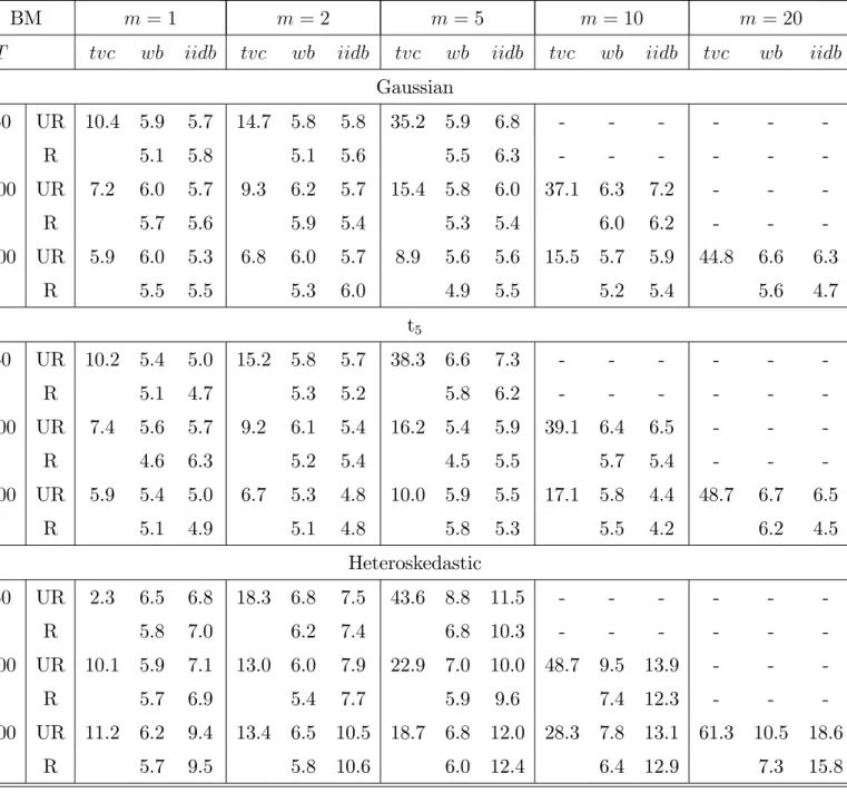
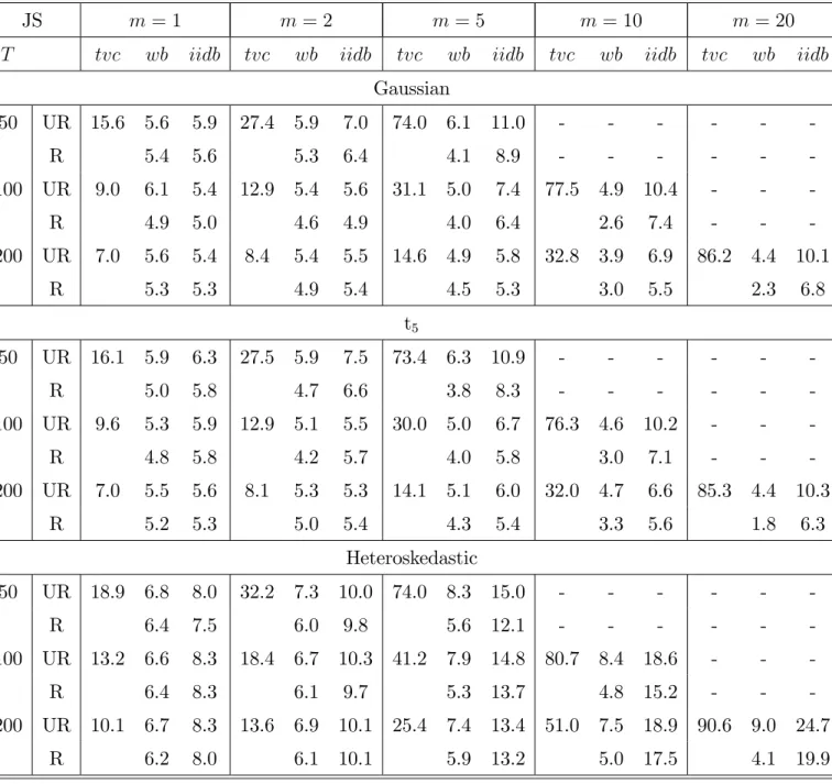
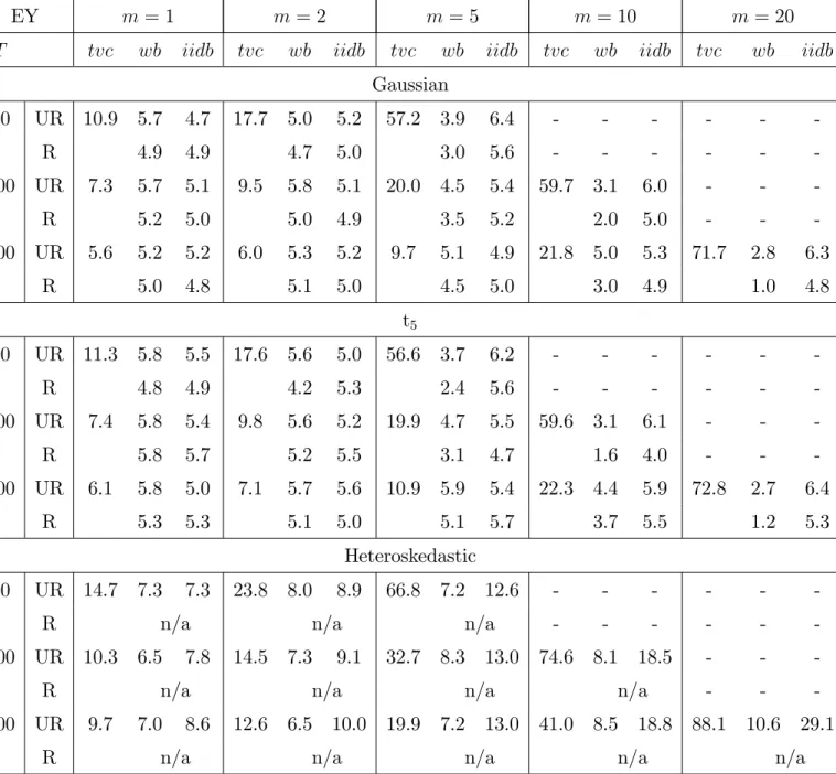
We seek to estimate the probability of rejecting the null hypothesis of TI cointegration when it is in fact true, for each of the three TVC tests described above and to observe how those results vary with m and T; besides p; r and k which change across DGP’s. The Tables 1 (BM model), 2 (JS model) and 3 (EY model) report the …nite-sample test-levels for each distributional approximation where tvc denotes the original TVC test against the chi-squared distribution and wb and sb refer to the wild and i.i.d. TVC tests, respectively, against the bootstrap distribution. The results based on the bootstrap procedure using the unrestricted residuals (and b) are presented at the right of label "UR" and those using the restricted ones at the right of "R". The results for tvc under t-distributed and heteroskedastic errors must be somehow read in careful under the original assumption of normality at Bierens and Martins (2010), although we conjecture that the result hold true when relaxing this distributional restriction.
The examination of the empirical properties of the original test illustrates the severity of the size distortions, especially for small T and large m; regardless of the DGP under consideration. For large m; the empirical size approaches the nominal one at the expense of a (much) higher number of observations. In contrast, the bootstrap tests provide in general near-exact levels for any combination of T or m: This fact is robust to any of the considered model speci…cations except for the conditional heteroskedasticity case with large m where real sizes of the i.i.d. bootstrap test are equal to about 10% or above. Regarding this particular setup, only the wild bootstrap test showed very reasonable results in general. This is somehow consistent with the …ndings at Cavaliere, Rahbek and Taylor (2010a).
In terms of the unrestricted and restricted approaches, we observe that the empirical size of the latter is always smaller than the former. For most cases, this implies having an empirical size (even) closer to the nominal 5% for the restricted procedure. But on the other hand, the Wild bootstrap under the restricted approach fails to reject the null too
often for m large and models JS and EY. Noticebly, the restricted procedure seems not to work for the EY model under conditionally heteroskedastic errors (contrary to models BM and JS, r = 2 at the EY model): the largest solution of the generalized eigenvalue
problem under the null and/or under the alternative, b0;1; bm;1; is systematically larger
than one for the simulated data, thus invalidating the calculation of the test statistic
(recall that it must hold true that 1 > bm;1 b0;1):
Hence, we advocate the usage of the bootstrap versions of the TVC test, namely the wild bootstrap using the unrestricted residuals, since these seem to be the only techniques that work well globally when testing for standard cointegration against TVC.
In a recent paper, Cavaliere, Taylor and Trenkler (2013) extend Swensen (2006) and Cavaliere, Rahbek and Taylor (2010a, 2012) by adapting Killian’s (1998) bootstrap-after-bootstrap (BaB) framework to their bootstrap-after-bootstrap-based LR cointegration rank tests. More speci…cally, bias-corrected VECM parameter estimates, obtained from the bootstrap repli-cations, are used instead to generate the pseudo-data and calculate the test statistic. Be-cause Cavaliere, Taylor and Trenkler’s standard cointegration model is the same as ours, we also implemented their algorithm to the TVC unrestricted bootstrap procedures in order to assess whether small sample gains can be obtained. The TVC BaB algorithm is the same as the one previously described with the following di¤erence: The estimated b0
js used to obtain the bootstrap sample 4Ytb
T
t=1 in step two, and consequently the LR
test statistic in step three, are replaced by the bootstrap bias-corrected estimates. That is, bj bbj = e b j 1 B B X b=1 eb j e b j ! ; j = 1; :::; p 1; where eb
j is the estimate based on the b th bootstrap sample. According to the Monte
Carlo results for model BM, there seems not to exist gains by implementing the BaB pro-cedure. In general, the empirical level increases slightly in both wild and i.i.d. bootstrap schemes and for all sample sizes. The only exceptions are: wb with m = 1 and T = 50 (drops from 5.9 to 5.7) and sb with m = 10 and T = 100 (a drop from 7.2 to 6.8).
Table 1: Empirical Sizes of Standard and Bootstrap TVC Tests for the BM model
BM m = 1 m = 2 m = 5 m = 10 m = 20
T tvc wb iidb tvc wb iidb tvc wb iidb tvc wb iidb tvc wb iidb
Gaussian 50 UR 10.4 5.9 5.7 14.7 5.8 5.8 35.2 5.9 6.8 - - - -R 5.1 5.8 5.1 5.6 5.5 6.3 - - - -100 UR 7.2 6.0 5.7 9.3 6.2 5.7 15.4 5.8 6.0 37.1 6.3 7.2 - - -R 5.7 5.6 5.9 5.4 5.3 5.4 6.0 6.2 - - -200 UR 5.9 6.0 5.3 6.8 6.0 5.7 8.9 5.6 5.6 15.5 5.7 5.9 44.8 6.6 6.3 R 5.5 5.5 5.3 6.0 4.9 5.5 5.2 5.4 5.6 4.7 t5 50 UR 10.2 5.4 5.0 15.2 5.8 5.7 38.3 6.6 7.3 - - - -R 5.1 4.7 5.3 5.2 5.8 6.2 - - - -100 UR 7.4 5.6 5.7 9.2 6.1 5.4 16.2 5.4 5.9 39.1 6.4 6.5 - - -R 4.6 6.3 5.2 5.4 4.5 5.5 5.7 5.4 - - -200 UR 5.9 5.4 5.0 6.7 5.3 4.8 10.0 5.9 5.5 17.1 5.8 4.4 48.7 6.7 6.5 R 5.1 4.9 5.1 4.8 5.8 5.3 5.5 4.2 6.2 4.5 Heteroskedastic 50 UR 2.3 6.5 6.8 18.3 6.8 7.5 43.6 8.8 11.5 - - - -R 5.8 7.0 6.2 7.4 6.8 10.3 - - - -100 UR 10.1 5.9 7.1 13.0 6.0 7.9 22.9 7.0 10.0 48.7 9.5 13.9 - - -R 5.7 6.9 5.4 7.7 5.9 9.6 7.4 12.3 - - -200 UR 11.2 6.2 9.4 13.4 6.5 10.5 18.7 6.8 12.0 28.3 7.8 13.1 61.3 10.5 18.6 R 5.7 9.5 5.8 10.6 6.0 12.4 6.4 12.9 7.3 15.8
Table 2: Empirical Sizes of Standard and Bootstrap TVC Tests for the JS model
JS m = 1 m = 2 m = 5 m = 10 m = 20
T tvc wb iidb tvc wb iidb tvc wb iidb tvc wb iidb tvc wb iidb
Gaussian 50 UR 15.6 5.6 5.9 27.4 5.9 7.0 74.0 6.1 11.0 - - - -R 5.4 5.6 5.3 6.4 4.1 8.9 - - - -100 UR 9.0 6.1 5.4 12.9 5.4 5.6 31.1 5.0 7.4 77.5 4.9 10.4 - - -R 4.9 5.0 4.6 4.9 4.0 6.4 2.6 7.4 - - -200 UR 7.0 5.6 5.4 8.4 5.4 5.5 14.6 4.9 5.8 32.8 3.9 6.9 86.2 4.4 10.1 R 5.3 5.3 4.9 5.4 4.5 5.3 3.0 5.5 2.3 6.8 t5 50 UR 16.1 5.9 6.3 27.5 5.9 7.5 73.4 6.3 10.9 - - - -R 5.0 5.8 4.7 6.6 3.8 8.3 - - - -100 UR 9.6 5.3 5.9 12.9 5.1 5.5 30.0 5.0 6.7 76.3 4.6 10.2 - - -R 4.8 5.8 4.2 5.7 4.0 5.8 3.0 7.1 - - -200 UR 7.0 5.5 5.6 8.1 5.3 5.3 14.1 5.1 6.0 32.0 4.7 6.6 85.3 4.4 10.3 R 5.2 5.3 5.0 5.4 4.3 5.4 3.3 5.6 1.8 6.3 Heteroskedastic 50 UR 18.9 6.8 8.0 32.2 7.3 10.0 74.0 8.3 15.0 - - - -R 6.4 7.5 6.0 9.8 5.6 12.1 - - - -100 UR 13.2 6.6 8.3 18.4 6.7 10.3 41.2 7.9 14.8 80.7 8.4 18.6 - - -R 6.4 8.3 6.1 9.7 5.3 13.7 4.8 15.2 - - -200 UR 10.1 6.7 8.3 13.6 6.9 10.1 25.4 7.4 13.4 51.0 7.5 18.9 90.6 9.0 24.7 R 6.2 8.0 6.1 10.1 5.9 13.2 5.0 17.5 4.1 19.9
Table 3: Empirical Sizes of Standard and Bootstrap TVC Tests for the EY model
EY m = 1 m = 2 m = 5 m = 10 m = 20
T tvc wb iidb tvc wb iidb tvc wb iidb tvc wb iidb tvc wb iidb
Gaussian 50 UR 10.9 5.7 4.7 17.7 5.0 5.2 57.2 3.9 6.4 - - - -R 4.9 4.9 4.7 5.0 3.0 5.6 - - - -100 UR 7.3 5.7 5.1 9.5 5.8 5.1 20.0 4.5 5.4 59.7 3.1 6.0 - - -R 5.2 5.0 5.0 4.9 3.5 5.2 2.0 5.0 - - -200 UR 5.6 5.2 5.2 6.0 5.3 5.2 9.7 5.1 4.9 21.8 5.0 5.3 71.7 2.8 6.3 R 5.0 4.8 5.1 5.0 4.5 5.0 3.0 4.9 1.0 4.8 t5 50 UR 11.3 5.8 5.5 17.6 5.6 5.0 56.6 3.7 6.2 - - - -R 4.8 4.9 4.2 5.3 2.4 5.6 - - - -100 UR 7.4 5.8 5.4 9.8 5.6 5.2 19.9 4.7 5.5 59.6 3.1 6.1 - - -R 5.8 5.7 5.2 5.5 3.1 4.7 1.6 4.0 - - -200 UR 6.1 5.8 5.0 7.1 5.7 5.6 10.9 5.9 5.4 22.3 4.4 5.9 72.8 2.7 6.4 R 5.3 5.3 5.1 5.0 5.1 5.7 3.7 5.5 1.2 5.3 Heteroskedastic 50 UR 14.7 7.3 7.3 23.8 8.0 8.9 66.8 7.2 12.6 - - -
-R n/a n/a n/a - - -
-100 UR 10.3 6.5 7.8 14.5 7.3 9.1 32.7 8.3 13.0 74.6 8.1 18.5 - -
-R n/a n/a n/a n/a - -
-200 UR 9.7 7.0 8.6 12.6 6.5 10.0 19.9 7.2 13.0 41.0 8.5 18.8 88.1 10.6 29.1
R n/a n/a n/a n/a n/a
4
Reassessing TV PPP
In Bierens and Martins (2010), the original TVC test statistic was applied to the pur-chasing power parity (PPP) hypothesis: In its absolute form, it means that the same bundle of goods, measured in real terms, should have the same value across countries. By taking the U.S.A. as the domestic country, Bierens and Martins (2010) concluded that price indices and nominal exchange rates are cointegrated, but in a TV fashion. Given the size distortions of the test and the accurate distribution approximation of the bootstrap versions of the test, in this Section, we reevaluate the PPP hypothesis using the same data as in Bierens and Martins (2010), but now computing the wild and i.i.d. bootstrap TVC test statistics as well, for both unrestricted (UR) and restricted (R) approaches.
4.1
PPP in the Context of TVC
The literature on the PPP hypothesis is recognizably vast and several reviews have
been proposed (see, for example, Taylor and Taylor, 2004). In our notation, Yt =
ln Stf; ln Ptn; ln Ptf 0
; where Ptn and P
f
t are the price indices in the domestic and
for-eign economies, respectively, and Stf is the nominal exchange rate in home currency per
unit of the foreign currency. Taking the symmetry and proportionality restrictions of
the absolute version of PPP, 0 = (1; 1; 1) ; is not expected to hold in empirical work
due to several aspects namely measurement errors of the price indices. Hence, the
tra-ditional empirical strategy assumes to be unknown and estimates the deviation series
from PPP, et = 0Yt; under the Engle and Granger (1987) or Johansen’s methodology,
= (1; 2; 3) : Under the assumption of no transactions costs, PPP requires that bet
follows a stationary process.
Whether it be the existence of transaction costs, nontradable goods, or market struc-tures with imperfect competition, it is highly unlikely that the equilibrium parity condition holds in its traditional representation. Due to the presence of such market frictions or measurement errors of the price indices in equilibrium models of real exchange rate de-termination, which may imply a nonlinear adjustment process in the PPP relationship, we test for the single constant cointegration hypothesis against our TVC speci…cation. The short run deviations from the PPP due to shocks in the system are measured by
et= 0tYt;where tis an unknown deterministic function of time that is approximated by
t(m) =
Pm
i=0 iPi;T (t) ; where the i’s are the Fourier coe¢ cients. Under the standard
PPP hypothesis (time-invariant cointegration), i = 0 for all i = 1; :::; m; for a …xed m:
The way to departure from the traditional Engle and Granger and Johansen’s ap-proaches might not be consensual. To put it simple, depending on the underlying model speci…cation and assumptions and the properties of the data, one may …t the PPP the-ory within an I(1) or I(2) framework; assume a linear or nonlinear type of cointegration model; and impose a set of coe¢ cients that are either …xed or time-varying (threshold cointegration, smooth transition, markov-switching, and so forth).
For example, Falk and Wang (2003) considered the PPP relationship within an I(1) framework whereas Johansen et al (2010) and Frydman et al (2008) argue that it …ts instead within the I(2) framework and thus making the standard approach possibly mis-leading. Based on rational expectations hypothesis sticky-price monetary models, the I(1) approach assume that nominal exchange rates and relative good prices are unit-root processes, while the real exchange rate is stationary (or a near-I(1) process). Instead, Johansen et al (2010) question these monetary models, specifying an I(2) model with piecewise linear trends where the change in real exchange rate is stationary but highly
persistent and apply it to German-USA data in the period 1975-1999.4 On the other
hand, Hong and Phillips (2010) propose a RESET-type test for linear against nonlinear cointegration and applied it to the PPP theory using UK-USA, Mexico-USA, Canada-USA and Japan-Canada-USA data from 1971 to 2004. They found little evidence for a linear relationship, except for the Mexico-USA case.
An important branch of the PPP literature assumes a nonlinear adjustment process in the …xed PPP cointegration relationship. It is argued that due to the presence of
transactions costs, the deviations from the PPP et= 0Yt is a nonlinear process that can
very well be characterized in terms of a smooth transition autoregressive model (ESTAR model). In this type of models, regime changes occur gradually rather than suddenly and the speed of adjustment varies with the extent of the deviation from parity. Typically,
the deviations from the PPP are obtained (i.e., estimated, bet = b
0
Yt) using the Engle
4Michael et al. (1997) also found German prices and nominal exchange rates to be I(2) processes
whereas non-German series are I(1). That is, German data seems to be a good empirical example where PPP holds within an I(2) approach.
and Granger (see Michael et al., 1997) or the Johansen’s cointegration method (see Baum et al, 2001). The results provide strong evidence of mean-reverting behavior for PPP deviations and against the linear framework.
It is known that testing for a linear speci…cation with time varying coe¢ cients against a nonlinear model with …xed parameters, or selecting the best out of the two, is not an easy task. Once we believe in Clive W. J. Granger’s assertion that “any non-linear model can be approximated by a time-varying parameter linear model” (Granger, 2008), we cannot reject a priori the relevance of a speci…cation such as the one we are considering in the paper.
As it just so happens with the nonlinear adjustment speci…cation, our model also as-sumes PPP cointegration in a nonstandard fashion, including the smooth transitions. In particular, the TVECM is able to empirically assess the strongest assumption in PPP
the-ory: The single cointegration vector being of the form = (1; 1; 1)and, correspondingly,
the real exchange rate a stationary process. This absolute version of the PPP hypothesis occurs if the null hypothesis of our TVC test is not rejected and, furthermore, the restric-tions are also not rejected. The bootstrap TVC test is shown to be a "good" statistical
tool to see if those changes around a constant are signi…cant or not.
Cheung and Lai (1993) claim that, due to transaction costs and measurement errors
in prices, if et is stationary and ( 2 < 0; 3 > 0) ; PPP holds. The Appendix to Bierens
and Martins’ paper includes the plots of the estimated bt: There, one can see that, in
general, bt seems to ‡uctuate around (1; 1; 1) and, in particular, t2 < 0; t3 > 0 for
most t: From an economic point of view, this means that the presence of market frictions and/or measurement errors of the price indices is the cause of time-varying adjustments
on the relative importance of each variable in Yt (nominal exchange rates and prices) to
guarantee stationary PPP deviations.5 That is, contrary to the former two-stage approach
(obtainbet= b
0
Ytand then …t a STAR model to it), at the TVECM, the PPP equilibrium
is directly restored via the cointegration vector, bt:
5As a simple example,
t = 1; 1 + cos(t)
T ; 1 ; t = 1; :::; T; ‡uctuates very closely to (1; 1; 1) and
satis…es t2 < 0; t3 > 0. In this case, slightly smaller importance in relative prices is given to the domestic economy.
4.2
Empirical Results
The data we use to illustrate the usefulness of the bootstrap TVC tests in empirical work is the same as in Falk and Wang (2003), downloaded from the Journal of Applied Econometrics data archives web site. For this particular dataset, they put the PPP
relationship within an I(1) framework.6 The U.S.A. bilateral relationship of study is with
the U.K., Japan, Canada, France, Italy, Germany, Belgium, Denmark, the Netherlands, Norway, Spain and Sweden. The data are monthly comprising 324 observations and cover the period from January 1973 to December 1999.
In this empirical application where a drift is included, k = 3 and r = 1; we consider m ranging from 1 to 32 = bT=10c : For the bootstrap tests, B = 399 and the initial values
Yb
t; t = p + 1; :::; 0; are set equal to the …rst observation in the sample, Y1: Just as in
Bierens and Martins (2010), the admissible values for the lag order include p = 1; 6; 10 and
18: Based on the Hannan-Quinn information criterion (HQ, Hannan and Quinn, 1979),
we took p = 1 which, for all reasonable m and countries, becomes the selected model over
p = 6; 10; 18:7
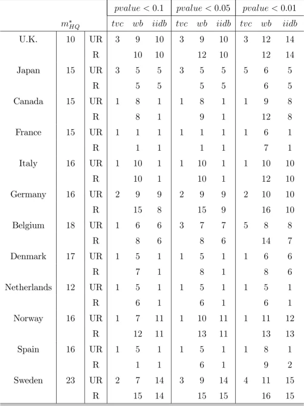
The results are presented in Table 2. The column labeled "mHQ" indicates the value
for m that is selected according to the HQ criterion. At its right, we …nd results for
1%; 5% and 10% levels (columns "pvalue<...") for each one of the three tests (tvc; wb
and sb): For a given test and signi…cance level, each number corresponds to an integerme
such that one cannot reject the standard PPP hypothesis for all m < m:e Also, one can
…nd evidence for TV PPP whenever m m:e The pvalues are not always monotonic with
respect to m: It is by comparing "mHQ"to the me0s; at its right, that we draw conclusions
6We also computed several unit root tests (including some more recent ones not in Falk and Wang,
2003) and con…rmed that nominal exchange rates are clearly I(1) and for the case of the price indices some evidence in favor of I(1) is found as well. Results available upon request.
7Apparently, in our TVECM, the HQ criterion tends to pick very large models and, consequently,
reducing drastically the degrees of freedom, as it happens with the AIC information criterion. In par-ticular, when m is relatively large, HQ chooses models with large values for p: For example, in the UK case HQ selects p = 1 rather than p = 6 for all m; rather than p = 10 for all m < 23; and rather than p = 18 for all m < 26: On the contrary, BIC always picks extremely small models, p = 1; m = 0; which becomes non-informative when testing for TVC. Therefore, to prevent from having models with m = 0 (BIC) or m close to bT =10c and p = 18 (huge loss of degrees of freedom), we set p = 1 and adopted the HQ criterion.
about the PPP hypothesis, for each bilateral relationship.
For the U.K., we …nd some evidence of a standard (TI) type of cointegration between U.K. and U.S.A. prices and the nominal exchange rate. According to Table 4 and for the
bootstrap tests at a 1% level, m > me HQ meaning that there is a wide range of possible
values for m such that one cannot reject the null hypothesis, including m that corresponds
to the selected model, according to HQ. At a 5% level,me is basically equal to mHQ:This
conclusion is, nevertheless, not shared by the remaining bilateral relationships where a TV cointegrating system is more likely to be true. That is, for all other countries, for any
test and signi…cance level, me is too small when compared to mHQ:
This empirical exercise shows the relevance of computing the bootstrap versions of the TVC test. It seems that the U.S.A. and the U.K. have kept a constant equilibrium relationship of prices and nominal exchange rates during the last quarter of the 20th
century.8 This is contradicted by the original TVC testing procedure.
5
Conclusion
In this paper we have considered two alternative bootstrap algorithms to the time-varying cointegration test proposed by Bierens and Martins (2010), based on a VECM speci…ca-tion where the cointegraspeci…ca-tion vector changes smoothly over time. The original likelihood ratio test and its wild and i.i.d. bootstrap versions have the same …rst-order asymptotic distribution under the null hypothesis of standard/time-invariant cointegration. Accord-ing to some extensive Monte Carlo simulations, and contrary to what happens with the original test statistic, the bootstrap procedures did not show severe size distortions. That is, the bootstrap approximation to the …nite-sample distribution can be considered very accurate, especially for the wild bootstrap case. We have applied the tests to the purchas-ing power parity hypothesis of international prices and nominal exchange rates with the U.S. as the home economy, and found evidence of standard cointegration in the U.S.A.-U.K. bilateral relationship and time-varying cointegration in the remaining eleven cases.
8In the standard Johansen’s cointegration context, the null hypothesis of symmetry and proportionality
Table 4: Standard and Bootstrap TVC Tests Applied to the PPP Hypothesis
pvalue < 0:1 pvalue < 0:05 pvalue < 0:01
mHQ tvc wb iidb tvc wb iidb tvc wb iidb
U.K. 10 UR 3 9 10 3 9 10 3 12 14 R 10 10 12 10 12 14 Japan 15 UR 3 5 5 3 5 5 5 6 5 R 5 5 5 5 6 5 Canada 15 UR 1 8 1 1 8 1 1 9 8 R 8 1 9 1 12 8 France 15 UR 1 1 1 1 1 1 1 6 1 R 1 1 1 1 7 1 Italy 16 UR 1 10 1 1 10 1 1 10 10 R 10 1 10 1 12 10 Germany 16 UR 2 9 9 2 9 9 2 10 10 R 15 8 15 9 16 10 Belgium 18 UR 1 6 6 3 7 7 5 8 8 R 8 6 8 6 14 7 Denmark 17 UR 1 5 1 1 5 1 1 6 6 R 7 1 8 1 8 6 Netherlands 12 UR 1 5 1 1 5 1 1 5 1 R 6 1 6 1 6 1 Norway 16 UR 1 7 11 1 10 11 1 11 12 R 12 11 13 11 13 13 Spain 16 UR 1 5 1 1 5 1 1 8 1 R 1 1 6 1 9 2 Sweden 23 UR 2 7 14 3 9 14 4 11 15 R 15 14 15 15 16 15
Note: Each entry below columns "pvalue<..." represents a value form (denote it asm);e such that for allm <me one cannot reject the null hypothesis.
The simplicity of application of the bootstrap TVC tests and their good performance in …nite-samples make the procedures discussed in this paper a valuable tool when address-ing the possibility for smooth time-transitions of the equilibrium relationship in several other examples of cointegrated variables. It is important to notice that the LR test setup is conditional on the existence of cointegration. An interesting topic that deserves fur-ther attention is how to test for "spurious" regression in our time-varying framework. The work by Park and Hahn (1999) in single-equation time-varying cointegration can be helpful in this respect.
References
[1] Andersson, S. A., H. K. Brons and S. T. Jensen (1983), Distribution of Eigenvalues in Multivariate Statistical Analysis, Annals of Statistics, 11, 392-415.
[2] Andrews, D. W. K. (1993), Tests for Parameter Instability and Structural Change with Unknown Change Point, Econometrica, 61, 821-856.
[3] Baum, C.F., J.T. Barkoulas and M. Caglayan (2001), Nonlinear Adjustment to Pur-chasing Power Parity in the Post-Bretton Woods Era, Journal of International Money and Finance, 20, 379-399.
[4] Bierens, H. J. (1994), Topics in Advanced Econometrics: Estimation, Testing and Speci…cation of Cross-Section and Time Series Models. Cambridge University Press. [5] Bierens, H. J. and L.F. Martins (2010), Time Varying Cointegration, Econometric
Theory, 26, 1453-1490.
[6] Brown, B.M. (1991) Martingale Central Limit Theorems, Annals of Mathematical Statistics, 42, 59-66.
[7] Cavaliere, G., A. Rahbek and A. M. R. Taylor (2010a), Cointegration Rank Testing Under Conditional Heteroskedasticity, Econometric Theory, 26, 1719-1760.
[8] Cavaliere, G., A. Rahbek and A. M. R. Taylor (2010b), Testing for Co-Integration in Vector Autoregressions With Non-Stationary Volatility, Journal of Econometrics, 158, 7-24.
[9] Cavaliere, G., A. Rahbek and A. M. R. Taylor (2012), Bootstrap Determination of the Co-Integration Rank in Vector Autoregressive Models, Econometrica, 80, 1721-1740. [10] Cavaliere, G., A. Rahbek and C. Trenkler (2013), Bootstrap Co-Integration Rank Testing: The Role of Deterministic Variables and Initial Values in the Bootstrap Recursion, Econometric Reviews, 32, 814-847.
[11] Cavaliere, G., A. M. R. Taylor and C. Trenkler (2013), Bootstrap Co-Integration Rank Testing: The E¤ect of Bias-Correcting Parameter Estimates, Working Paper 13-06, University of Mannheim, Department of Economics.
[12] Cheung, Y. and K.S. Lai (1993), Long-Run Purchasing Power Parity during the Recent Float, Journal of International Economics, 34, 1811-1192.
[13] Diebold, F. and C. Chen (1996), Testing Structural Stability with Endogenous Break Point: A Size Comparison of Analytic and Boostrap Procedures, Journal of Econo-metrics, 70, 221-241.
[14] Engel, R. F. and C. W. J. Granger (1987), Cointegration and Error Correction: Representations, Estimation and Testing, Econometrica, 55, 251-276.
[15] Engle, R. F. and B. S. Yoo (1987), Forecasting and Testing in Co-Integrated Systems, Journal of Econometrics, 35, 143-159.
[16] Falk, B. and C. Wang (2003), Testing Long Run PPP with In…nite Variance Returns, Journal of Applied Econometrics, 18, 471-484.
[17] Frydman, R., M. D. Goldberg, S. Johansen and K. Juselius (2008), A Resolution of the Purchasing Power Parity Puzzle: Imperfect Knowledge and Long Swings, Discussion Papers 08-31, University of Copenhagen. Department of Economics. [18] Granger, C. W. J. (2008), Non-Linear Models: Where Do We Go Next - Time Varying
Parameter Models? Studies in Nonlinear Dynamics & Econometrics, 12, issue 3, Article 1.
[19] Hannan, E. J., and C. C. Heyde (1972), On the Limit Theorems for Quadratic Functions of Discrete Time Series, Annals of Mathematical Statistics, 43, 2058-2066.
[20] Hannan, E. J., and B. G. Quinn (1979), The Determination of the Order of an Autoregression, Journal of the Royal Statistical Society B, 41, 190-195.
[21] Härdle, W., J. L. Horowitz and J.-P. Kreiss (2001), Bootstrap Methods for Time Series, Discussion Papers, Interdisciplinary Research Project 373: Quanti…cation and Simulation of Economic Processes, No. 2001,59.
[22] Harris, R. I. D. and G. Judge (1998), Small Sample Testing for Cointegration Using the Bootstrap Approach, Economics Letters, 58, 31-37.
[23] Hong, S.H. and P.C.B. Phillips (2010), Testing Linearity in Cointegrating Relations With an Application to Purchasing Power Parity, Journal of Business and Economic Statistics, 28, 96-114.
[24] Horowitz, J.L. (2001), The Bootstrap. In Heckman, J.J. and Leamer, E.E. (eds), Handbook of Econometrics, vol. 5, Chap. 52, 3159-3228, Elsevier Science B.V. [25] Jeong, J. and G.S. Maddala (1993), A Perspective on Application of Bootstrap
Meth-ods in Econometrics. In Handbook of Statistics, vol. 11, 573-610, North Holland Publishing Co.
[26] Johansen, S. (1988), Statistical Analysis of Cointegration Vectors, Journal of Eco-nomic Dynamics and Control, 12, 231-254.
[27] Johansen, S. (1991), Estimation and Hypothesis Testing of Cointegration Vectors in Gaussian Vector Autoregressive Models, Econometrica, 59, 1551-1580.
[28] Johansen, S. (1995), Likelihood-Based Inference in Cointegrated Vector Autoregressive Models. Oxford University Press.
[29] Johansen, S. (2002), A Small Sample Correction of the Test for Cointegrating Rank in the Vector Autoregressive Model, Econometrica, 70, 1929-1961.
[30] Johansen, S, K. Juselius, R. Frydman and M. D. Goldberg (2010), Testing Hypotheses in an I(2) Model with Piecewise Linear Trends an Analysis of the Persistent Long Swings in the dmk/$ Rate, Journal of Econometrics, 158, 117-129.
[31] Killian, L. (1998), Small-Sample Con…dence Intervals for Impulse Response Func-tions, Review of Economics and Statistics, 80, 218-230.
[32] Li, Hongyi and G.S. Maddala (1996), Bootstrapping Time Series Models, Economet-ric Reviews, 15, 115-158.
[33] Mantalos, P. and G. Shukur (2001), Bootstrapped Johansen Tests for Cointegra-tion RelaCointegra-tionships: A Graphical Analysis, Journal of Statistical ComputaCointegra-tion and Simulation, 68, 351-371.
[34] Martins, L.F. and V.J. Gabriel (2013), Time-Varying Cointegration, Identi…cation, and Cointegration Spaces, Studies in Nonlinear Dynamics and Econometrics, 17, 199-209.
[35] Michael, P., A. R. Nobay and D. A. Peel (1997), Transactions Costs and Nonlinear Adjustment in Real Exchange Rates: An Empirical Investigation, Journal of Political Economy, 105, 862-879.
[36] Paparoditis, E. P. and D. N. Politis (2003), Residual-Based Block Bootstrap for Unit Root Testing, Econometrica, 71, 813-855.
[37] Park, J. Y. (2003), Bootstrap Unit Root Tests, Econometrica, 71, 1845-1895.
[38] Park, J. Y. and S.B. Hahn (1999), Cointegrating Regressions with Time Varying Coe¢ cients, Econometric Theory, 15, 664-603.
[39] Swensen, A. R. (2006), Bootstrap Algorithms for Testing and Determining the Coin-tegration Rank in VAR Models, Econometrica, 74, 1699-1714.
[40] Swensen, A. R. (2006), Supplement to "Bootstrap Algorithms for Testing and De-termining the Cointegration Rank in VAR Models", Econometrica Supplementary Material 74.
[41] Swensen, A. R. (2009), Corrigendum to "Bootstrap Algorithms for Testing and De-termining the Cointegration Rank in VAR Models", Econometrica 77, 1703-1704. [42] Taylor, A. and M.P. Taylor (2004), The Purchasing Power Parity Debate, Journal of
[43] Trenkler, C. (2009), Bootstrapping Systems Cointegration Tests With a Prior Ad-justment for Deterministic Terms, Econometric Theory, 25, 243-269.
[44] van Giersbergen, N. P. A. (1996), Bootstrapping the Trace Statistics in VAR Models: Monte Carlo Results and Applications, Oxford Bulletin of Economics and Statistics, 58, 391-408.