1Department of Physics of the Earth and Environment, Institute of Physics, Universidade Federal da Bahia – UFBA, Salvador (BA), Brasil. E-mail: [email protected] 2Department of Geophysics, Institute of Astronomy, Geophysics and Atmospheric Sciences, Universidade de São Paulo – USP, São Paulo (SP), Brasil. E-mail: [email protected]; [email protected]
*Corresponding author
Manuscrito ID 30043. Recebido em: 07/10/2013. Aprovado em: 09/06/2014. ABSTRACT: he Goiás Alkaline Province (GAP), located on the north edge of the Paraná Basin, has alkaline complexes with strong magnetic signatures. he 3D inversion of magnetic signal was per-formed on the aeromagnetic data. Since the intrusions present a strong remnant magnetization, as measured in the laboratory, a care-ful analysis of this component was also realized. he sum vector of the remnant and induced components were used as a virtual induced magnetic ield during the 3D inversion process. he geometric pa-rameters were obtained from the quantitative analysis of magnetic data, using Total Gradient Direction and Analytical Signal Phase, performed over magnetic signal reduced to the pole. Magnetic sus-ceptibility and density were measured in laboratory. All this infor-mation were used as the initial model in the inversion. he results of 3D inversion show that the alkaline intrusions have roots up to 10-12 km depth. he magnetic susceptibility is distributed in almost spherical and cylindrical shapes. he possibility of spherical shapes arise the hypothesis that the GAP intrusions at the northern part of the province represent magmatic chambers. he alkaline magma as-cends from the lithosphere, and used two main fault systems as space for emplacement. hese faults systems appear in the magnetic signal analysis as linear magnetic features. Chemical analysis conirmed the alkaline and subalkaline character of the magmas. he high MgO content shows the primitive character of these intrusions but the Ba anomaly indicates a possible crustal contamination.
KEYWORDS: Alkaline magmatism; magnetic data; remnant magnetization; 3D inversion.
RESUMO: A Província Alcalina de Goiás (PAGO), localizada na borda norte da Bacia do Paraná, tem complexos alcalinos com fortes assinatu-ras magnéticas. A inversão do sinal 3D magnética foi realizada nos dados de magnetometria. Amostras coletadas em campo de algumas dessas in-trusões alcalinas apresentam forte magnetização remanescente, como mos-tram as medidas tomadas em laboratório, assim, uma análise cuidadosa desta componente também foi realizada. O vetor soma dos componentes remanescente mais induzidas foram usadas como um campo magnético induzido virtual durante o processo de inversão 3D dos dados magnéticos. Os parâmetros geométricos foram obtidos a partir da análise quantitativa de dados magnéticos, usando Gradiente Horizontal Total e Fase dos Sinal Analítico. As Susceptibilidades magnéticas e densidades foram medidas em laboratório. Todas as informações foram utilizadas como modelo inicial para a inversão. Os resultados da inversão 3D mostram que as intrusões alcalinas têm raízes até 10-12 km de profundidade. A susceptibilidade magnética é distribuída em formas quase esféricas e cilíndricas. A possibi-lidade das formas esféricas ocorre da hipótese de que as intrusões da GAP na parte norte da província representam câmaras magmáticas. O magma alcalino ascendeu da litosfera e usou dois principais sistemas de falhas como caminho preferencial para sua colocação. Estes sistemas de falhas aparecem na análise do sinal magnético como feições magnéticas lineares. A análise química conirmou o caráter alcalino e subalcalino dos magmas. O alto teor de MgO mostra o caráter primitivo dessas intrusões, mas a anomalia Ba indica uma possível contaminação crustal.
PALAVRAS-CHAVE: Magmatismo alcalino; dados magnéticos; magnetização remanescente; inversão 3D.
Aeromagnetic and physical-chemical
properties of some complexes from Goiás
Alkaline Province
Dados aeromagnéticos e Propriedades físico-químicas de
alguns complexos da Província Alcalina de Goiás
Alanna C. Dutra1*, Yára R. Marangoni2, Ricardo I. F. Trindade2
INTRODUCTION
he North border of the Paraná Basin, in Central Brazil, is characterized by an erosive scenario very active during the Upper Cretaceous with the intrusion of alkaline magmatism in the area. hree provinces are found, Goiás Alkaline Province, Alto Paranaíba Igneous Province and Porixoréu Province. his magmatism is set in groups of intrusions in Goiás, Minas Gerais and Mato Grosso states, some hundreds of kilometers apart. he intrusions are disposed in linear arrangements par-allel or with diferent angles in relation with the basin border, sometimes inside the basin and sometimes just outside it. he provinces shows similarities and diferences in the magma type, some of the intrusions have carbonatites, but share a very similar geophysical signature: high Bouguer anomalies and strong magnetic signal.
he Goiás Alkaline Province (GAP) is located in Goiás State, at the Paraná Basin border and in terrains of Bom Jardim de Goiás Volcanic Arc and other Precambrian ter-rains, it occupies an area of 250 x 70 km. he province pres-ents diferent magma sets: the north part is characterized by alkaline maic ultramaic intrusions, sub volcanic alka-line intrusions at the central portion and volcanic lows in the south part (Fig. 1). he alkaline complexes of the north region are intrusive and present diferent sizes. he main lithotypes found in the intrusions are dunites, peridotites, diverse pyroxenites, gabbro, alkali-gabbro, nepheline syenite and fenitization products. At the central and south por-tions it is easy to found dikes, sills and lava lows disposed in a linear band at the NW-SE direction. hese structures might take advantage of faults in that direction during their emplacement (Junqueira-Brod et al. 2002). he intrusive alkalines at the north part are the Morro do Engenho, Santa Fé, Montes Claros de Goiás, Arenópolis, Buriti, Córrego dos Bois e Morro do Macaco. he subvolcanics at the central part and lava lows at south are the Amorinópolis, Águas Emendadas and Santo Antônio da Barra. All of them are numbered in the map of Fig. 1.
he Precambrian terrains that host part of the GAP is composed of volcano-sedimentary sequences, granites and orthogneiss, post tectonic intrusions of diorite gab-bro and granite. he orthogneiss are mainly granite and granodiorite calco alkaline with high K, they show very restrict tonalites facies. he most NW intrusions cut Furnas Formation from Paraná Basin. his formation is of coarse sandstones of Devonian.
he GAP intrusions have a strong magnetic and gravi-metric signal. hey are so characteristic that some anoma-lies that have no related outcrop have been inferred as signal of subsurface intrusive. he lithology of the maic intrusive are appropriate for the strong geophysical signal because of
the comparatively high density and magnetite content com-pared with the surrounding geology. he magnetic signal was used to infer the distribution of magnetic susceptibil-ity in depth and constrain possible geometry for the intru-sives. he choice method of study was the 3D inversion constrained by results of application of Analytical Signal Phase and Horizontal Total Gradient. A careful analysis of magnetic properties was also made to determine possible remnant magnetization component.
The magnetic inversion may not be possible if the magnetic signal carries a remnant component. he rem-nant magnetization can change the interpretation of the geological source since it inluence the magnetic anom-aly. he efects of this component have been studied in detail by Brooks (1962) and Roest and Pilkington (1993), among others. he problem appears when the total mag-netization direction is unknown and diferent from the induced ield at the survey time. he possibility to over-come this common situation is to determine the remnant component in a laboratory and to work with the sum of the induced and remnant. In this work the sum vector was considered the virtual ield direction, in the sense that it substitutes the induced ield. he results obtained in the inversion proved that this is a feasible way to work with magnetic data when remnant magnetization is present.
PHYSICAL-CHEMICAL
ANALYSIS RESULTS
84 samples were collected from 8 sites in the studied region, all of them marked in Figure 1. Density (g/cm3) and
magnetic susceptibility (SI) are shown in Figure 2. he mean density value was 2.71 g/cm3, a value lower than expected
for the samples lithology. he mean magnetic susceptibil-ity was 0.02 (SI). Samples dunite (01) and syeno-diorite (09A) show strong weathering and are altered, that may be responsible for the low density values observed. hese values were considered despite the low density values because the samples show good results as the values of magnetization and magnetic susceptibility, and has been veriied by optical microscope that the magnetic minerals are well preserved in the samples. Despite this alteration the magnetic property is preserved, since they have high iron and magnesium oxides content as geochemical analysis conirmed.
Figure 1. Geological map of Goiás Alkaline Province (Brod et al. 2005). Cenozoic cover
Creataceous alkaline rocks Paleozoic-cretaceous (Parana Basin) Precambiam basement River
1) Morro de Engenho 2) Santa Fé
3) Montes Claros 4) Diorama 5) Córrego dos Bois 6) Morro do Macaco 7) Fazenda Buriti 8) Arenópolis 9) Amorinpolis 10)Águas Emendadas
11) Santo Antônio da Barra 12) A2 anomaly
13) Registro Araguaia anomaly Fault
Road City
Buried bodies Samples
-18º -17º -16º -50º -51º
-52º
12
13 1
2
3
4
5
6 8
7
9
10
Figure 3 shows de result from chemical analysis in a TAS dia-gram with alkaline and sub-alkaline rocks ields deined by Cox
et al. (1979). In the same igure are the results from previous work at the GAP made by Junqueira-Brod et al. (2005), grey circles. It is possible to see that the collected samples present similarities with previous works.
Some samples present high concentration of Ni (> 100 ppm) and Cr (> 1000 ppm) that coexist with high concentration of lithophile elements, like Zr (between 43.9 – 436.3 ppm), Sr (between 175.7 – 1139.9 ppm), Ba (between 59.2 – 3500.8 ppm). he Ba anomaly is a strong characteristic of a variety of intra-continental magmatism and can be attributed to the phlogo-pite presence in the mantle source or crustal contamination. he fractioning of light rare earth elements (REE) can be inter-preted as a result of high content of clinopyroxene and phlogo-pite in the melts. he high content of Cr (120 – 6660.6 ppm) and Ni (336 – 9251.4 ppm) are consistent with the ultramaic composition of the samples; particularly Ba, Sr and REE’s sum go to a few decimals of one percent. Nb (5 – 123 ppm) and Zr (44 – 436 ppm) concentrations are relatively high.
AEROMAGNETIC DATA
A new data set of aerogeophysical survey, magnetic and radiometric data, is available for Goiás State, Central Brazil.
Figure 2. Plot of density (g/cm3) and magnetic susceptibility (SI) of GAP samples.
3.400
3.200
3.000
2.800
2.600
2.400
2.200
2.000
density (g/cm
3)
0.00 0.02 0.04
magnetic susceptibility (SI)
0.06 0.08 0.10 0.12 gabbro
alkali granite gabbro syeno-diorite dunite dunite dunite
Table 1. Chemical analysis results from major (%) and trace (ppm) elements. Measurements were done with Spectrometry X-Ray Fluorescence using melted matrix of borate. Trace elements were analyzed in pressed samples.
Sample 01 06 09A 09B 09C 10A 10B
SiO2 45.00 46.15 51.48 68.29 47.20 43.15 39.43
TiO2 0.13 1.61 2.44 0.58 3.43 3.97 4.70
Al2O3 0.51 16.96 15.40 14.29 14.29 7.41 9.58
Fe2O3t 14.56 12.80 10.77 5.39 11.17 13.88 14.97
MnO 0.18 0.19 0.18 0.11 0.20 0.22 0.23
MgO 38.25 7.80 4.25 0.61 3.83 13.23 11.77
CaO 0.03 11.73 7.14 2.18 9.81 16.03 13.19
Na2O 0.21 2.36 3.63 3.47 2.14 0.88 2.83
K2O 0.11 0.23 4.09 4.90 7.16 0.66 2.50
P2O5 0.01 0.17 0.61 0.17 0.79 0.57 0.82
Cr 6660.0 196.7 114.6 145.7 28.8 1854.9 453.0
Ni 9251.4 91.5 19.0 8.1 8.6 336.0 146.6
Ba 86.9 56.2 1046.8 965.8 840.5 3500.8 1308.5
Rb 23.1 5.5 81.9 165.5 47.4 100.3 66.8
Sr -- 440.9 870.5 176.2 619.7 343.8 1139.9
La -- 3.6 79.3 66.5 62.6 44.3 73.7
Ce 203.7 16.8 78.6 88.6 -- 256.3 110.4
Zr 43.9 103.2 392.9 436.3 297.4 195.8 279.8
Y 57.8 30.0 32.0 36.9 32.3 10.5 20.3
Nb 0.68 4.6 77.6 17.8 123.4 -- 94.1
Cu -- 54.5 8.5 10.8 5.4 28.7 54.8
Zn 105.6 115.8 92.8 96.8 93.0 44.3 90.2
Most of the GAP region has been surveyed in 2004 at the irst stage of the project. he area was lown at a height of 100 m, with line 0.5 km apart at the NS direction with ten measurements at 0.1 s interval. Control lines were in the EW direction 5 km apart. Survey was positioned with GPS precision better than 10 m (LASA 2004). he used parameters imply that anomalies with spatial dimensions less than 1 km (twice the interval of sample proile) can not be well represented (Telford et al. 1990, Blakely 1996). Data processing included corrections for diurnal variation, parallax error, leveling and microleveling of proiles and removal of IGRF calculated at light height referred to year 2000 and at the date of August 2004. he inal available product is the total ield magnetic anomaly (as shown in Fig. 4). Details of all the stages involved in the aeromag-netic survey and ield data treatment can be found in the survey rapport (LASA 2004).
he interpolation method used was bidirectional, with the grid spacing of 125 x 125 m2. he line direction is very
close to either north-south, this approach will also enhance
geological trends perpendicular to the line direction. Since we ideally want to enhance features perpendicular to the survey line direction, we should specify this angle to be per-pendicular to the line direction.
In Fig. 4 the GAP intrusions show a strong magnetic anomaly. It is remarkable the coincidence between the two geophysical signals and the high amplitude that they have for most of the outcrops. Both signals display anomalies almost circular over the GAP intrusions. Magnetic anom-alies have diameters in the order of 10 km and lineaments are longer than 20 km indicating that both type of struc-tures referred to intrusions with considerable size located at the upper and medium crust. he expected aliasing efect because of the distance between plane and intrusions top is about 20% (Reid 1980) since most part of the intrusions are exposed. his efect may be considerable and some part of the signal could be lost, but as the anomalies are exten-sive and have been surveyed by a few light lines (5 or more) it is reasonable to consider that the map of Fig. 4 shows a good relationship with the geological situation in the area. he quantitative analysis of the magnetic data was per-formed in the frequency domain. To avoid border efects the grid was enlarged at their borders by 10% with val-ues extrapolated from the original grid. Frequencies above Nyquist number, 1.9 cycle/km in the area, were eliminated since they may represent noise.
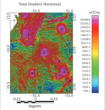
It was calculated the Total Horizontal Gradient (THG) and Analytical Signal Phase (ASP) of the total anomaly magnetic ield. Applications of these two techniques help to infer geometry and size of the magnetic fonts. he work
15
13
11
9
7
5
3
1
14
13 12
11 15
10
6 9
8 7
5 4
3 2 1 37
Na2O+K2O wt%
Si2O wt%
41 45 49 53 57 61 65 69 73
Figure 3. Diagram of SiO2 versus (N2O + K2O (TAS: Le Maitre 1989, Le Bas et al. 1986). The gray line divides the sub-alkaline series from the alkaline series (high alkalies). Black circles, this work; grey circles, ater Junqueira-Brod et al. 2005; red squares, ater Brod et al. 2005. Nomenclature (in parethesis the intrusive equivalent): 1, picrobasalt (ultramaite); 2, basalt (gabbro); 3, basaltic andesite (diorite); 4, andesite (Qz-diorite); 5, dacite (granodiorite); 6, rhyolite (granite); 7, trachybasalt (monzogabbro); 8, basaltic trachyandesite (monzodiorite); 9, trachyandesite (monzonite); 10, trachyte, if quartz < 20% (Qz-monzonite), trachydacite if quartz > 20% (syenite); 11, tephrite if olivine < 10% (foid bearing monzogabbro), basanite if olivine > 10% (foid bearing gabbro); 12, phonotephrite (foid bearing monzodiorite); 13, tephrifonolite (foid bearing monzosyenite); 14, phonolite (foid syenite); 15, foidite (foidolite).
Total Field Magnetic Anomaly
degrees
0.25 -51.50 0.25 -51.0
-51.5 -51.0
-16.5
-16.5
-16.0
-16.0
-15.5
-15.5 (nT) 1242.9
365.5 211.3 143.0 106.0 81.6 64.7 52.2 42.8 35.7 30.1 24.2 18.1 13.2 8.8 4.5 0.1 -4.4 -9.0 -13.9 -19.5 -25.8 -33.1 -41.4 -50.8 -62.0 76.8 -95.8 -122.2 -175.6 -321.7 -909.8
hypothesis is that the peaks of the signal amplitude are orig-inated by vertical contacts and, in this case, the anomaly width is proportional to its depth. he results obtained are show in Fig. 5. he THG and ASP were performed over the total magnetic anomaly reduced to the pole. In Fig. 5 it is possible to notice that each anomaly results from an isolated intrusion (or body when there is not an outcrop), the limits are marked and results in almost circular shape. Magnetic lineaments were also enhanced and are mostly in the NW-SE direction except close to anomaly 12 (Registro do Araguaia) where a striking NE-SW lineament marks the north part of the inferred intrusion and extends behind the limits of the area. his region is totally recovered by quaternary sediments from the Araguaia River. It is interesting to note that the NW-SE features cross some of the anomalies but does not deform it, as can be seen in the anomalies 3 (Montes Claros) and 5 (Córrego dos Bois). Some of these lineaments also show relation with mapped faults in the area.
he alkaline provinces show a clear tectonic control of magmatism by crustal discontinuities mainly extensional or wrenching fault zones (magnetic lineaments) along the present-day borders of sedimentary basins (magnetic signal with smoothed relief ). Inheritance of Proterozoic crustal discontinuities have played a major role on the alkaline magmatism. Changes in the stress-ields and reactivations of regional structures in diferent pulses produced a great range of structural weakness along which alkaline magmas were emplaced or reached the surface. hese tectonic con-trols explain the regional distribution of alkaline magmatism in the central-southeastern region of the Brazilian Platform.
MAGNETIC PROPERTIES
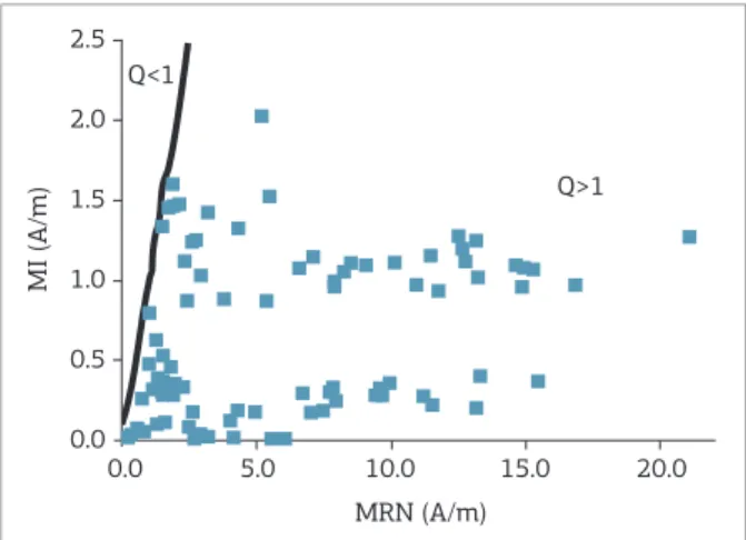
GAP intrusion show a strong magnetic anomaly com-posed of induced (Mi) and remnant (MR) magnetization, as has been already discussed by Dutra and Marangoni (2009). Since the remnant magnetization is very strong it was nec-essary to collect oriented samples and to determine their remnant magnetic properties. Figure 8 shows a plot of the magnetization components. In this Figure it is possible to observe that almost all of them have Konigsberger ration (Q) greater than one and just a few have Q = 1, that emphasizes the importance of the remnant component.
In order to determine remnant magnetization direction, measurements were done on 84 cylinders of oriented ield samples collected in the area (location of site samples are in Figure 1 as solid triangles). he samples were collected with a gasoline portable drill hole, water cooled, with diamond drill that cut cylindrical samples of 2.5 cm in diameter. he samples were oriented in the magnetic ield using a leveled
compass so magnetic azimuth and inclination angle could be determined. he volumetric magnetization was mea-sured in a magnetometer of the Paleomagnetic Laboratory of Institute of Astronomy, Geophysics and Atmospheric Science of the Universidade de São Paulo (IAG-USP) and results in the sample referential system were them translated into local geographical sample.
Natural Remnant Magnetization (NRM) determina-tions include primary magnetization acquired at the time of rock formation and secondary magnetizations acquired after rock formation. It is important to remove the sec-ondary magnetization to better determine the direction of the ield at the time of the cooling of the alkaline intru-sions. Two diferent techniques were applied to remove this information: (a) alternated magnetic ield and (b) thermal demagnetization.
In the application of alternate magnetic ield, the cycle begins with the induced magnetic ield at the maximum intensity H and inishes at zero ields; at the end the exist-ing magnetization is measured. When the induced magnetic ield reaches H the magnetic moment of the grain whose coercivity is minor or equal to H will align at the same ori-entation of the applied magnetic ield. When the ield inten-sity goes to zero the magnetic grain loose its orientation and total magnetization will be equal to zero. here is a direct relationship between the intensity of the applied magnetic ield and the mineral coercivity (Tauxe 2002).
In the case of demagnetization by thermal process it is possible to investigate the spectrum of blocking tem-perature (and its mineral composition) by heating the
Total Gradient Horizontal
degrees
0.25 -51.50 0.25 -51.0
-51.5 -51.0
-16.5
-16.5
-16.0
-16.0
-15.5
-15.5 (nT/m)
65068.8 35105.2 24320.0 18574.0 14815.7 12208.9 10217.5 8687.3 7407.7 6295.5 5351.0 4546.5 3805.9 3145.5 2556.5 2018.1 1513.3 1026.1 506.1
sample at monotonic increasing temperatures and mea-suring the magnetization after the cooling process for each step. he whole process — heating and cooling — is carried out in a zero magnetic ield. he blocking tem-perature of each mineral is known and very stable until temperature is close to Curie point, so it is possible to determine the main magnetic minerals present at the sample and observe secondary magnetizations that are removed at lower temperature. After the rock is cooled only the MRN is present.
he remnant directions are calculated using the primary component. It is given the same weight to a point sequence that corresponds to an individual component. he direction of the characteristic remnant magnetization is calculated by least square method for the most stable directions measured. he mean direction is calculated using Fisher’s statistics (Fisher 1953). It considers all N vectors whose intensity is equal to one and the mean of directions < S→> equal to the vectorial sum (< R→ >) of the all N vectors divided by their intensity R (< S→> = R→ / R). Fisher (1953) suggests some statistical parameters to deine the data groups and reliabil-ity of the mean direction obtained. he precision parameter
K deines the direction dispersion over a sphere of unitary radius. he best estimate for the value of K (for N > 3) is given by the relation: K = [(N-1) / (N-R)]. he obtained directions will be grouped if N is close to R (i.e. K has a high value). If the data dispersion is very high then R will be smaller than N and K parameter will have a low value. he angle α95 ≈ 140º/√KN is another parameter that may be considered. It represents twice the standard deviation using spherical projection.
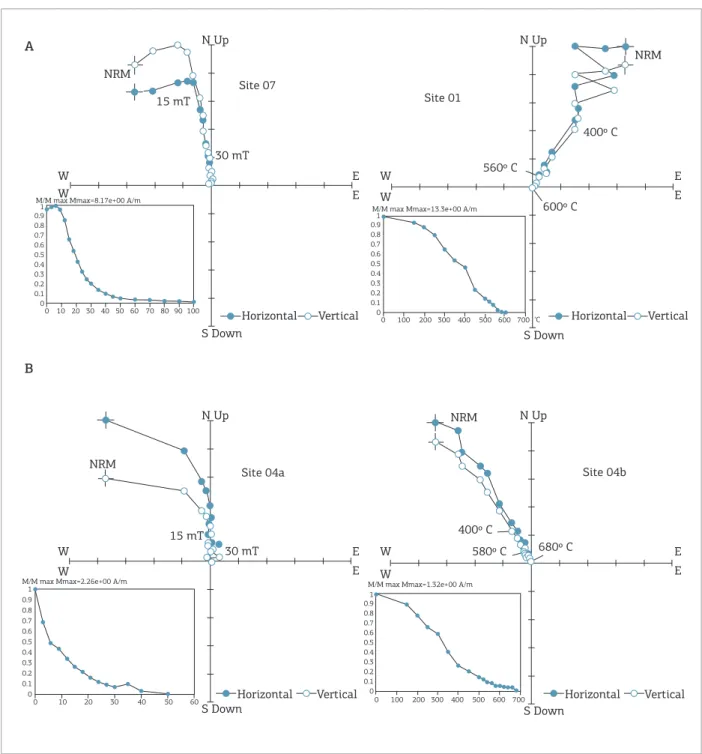
he populations of MNR magnetizations directions that follow Fisher’s density distribution function were isolated with the two demagnetization processes, alter-nate ields and thermal process. he analyzed samples showed multiple components that were very well deined in orthogonal directions. For the samples majority the less stable components were isolated between 0 – 20 mT on average (Fig. 6A). In the thermal demagnetization the less stable components were isolated between 0 and 600 oC on average (Fig. 6B). hose components were
interpreted as secondary remnant magnetization acquired after rock cooling.
Figure 7presents the magnetization direction (decli-nation and incli(decli-nation at the local geographic reference system) using stereographical projection. Two groups are deined in the igure. One composed by south direction and negative inclination represented by samples 01, 04, 07 and 10, located at most north area of the GAP. Figure 6 shows examples of demagnetization results of this component. he second group has direction pointing towards north
with positive inclination. hey were found at sites 06, 09A and 09B located at the central part of the GAP. It was not possible to complete isolate the primary remnant magne-tization using alternate ields for samples from site 09. So, in a later step samples from this site were submitted to the thermal demagnetization. his process was also applied to a few specimen of each site.
he mean magnetization direction for each site was calcu-lated using just the specimens that presented coherent mag-netizations and acceptable statistical parameters (Fig. 7B), that is, sites 01, 04 and 07. Table 2 presents a summary with the mean direction and statistical parameter for each site. he mean values of susceptibility and magnetic direction were used in the reference models for the inversion proces-sion of GAP aeromagnetic data.
3D INVERSION OF MAGNETIC DATA
he anomalous ield produced by the distribution of magnetization J = Jx,Jy,Jz is given by the following integral equation with a dyadic Green’s function:
∫ ·
-∇∇
V r r Jdv
= r T
' 1 4
) ( 0
π
μ
→ →
→ → (1)
where µ0 = 1 is the magnetic permeability, T(xi,yi,zi) is the observation of the jth rectangular prism, and r is the posi-tion of the observaposi-tion point. V represents the volume of magnetization (MAG3D 2002).
In 3D inversion the source and substrate are discretized into M cells, and each cell has uniform magnetization. he observations T(xi,yi,zi) are approximated by a contin-uous function, the integrals of equation (1), expressing
2.5
2.0
1.5
1.0
0.5
0.0
MI (A/m)
MRN (A/m)
0.0 5.0 10.0 20.0
Q>1 Q<1
15.0
the relationship between the physical property, magnetic susceptibility, and the corresponding magnetic observa-tions. Some methods use a linear formulation for the inverse problem and, in this case, divide the subsurface into a set of prismatic cells with known size and posi-tion, but with contrasting physical property unknown. he interpretive model consist of 3D prisms juxtaposed with constant magnetic susceptibility into each prism
to be determined. he distribution of magnetization in these blocks delineates the magnetic source in the region generating the total ield anomaly observed, represented by equation (1).
Li and Oldenburg (1996) developed an inversion technique to determine the distribution of magnetic susceptibility. hey considered that the model is directly proportional to the magnetic ield anomaly and varies on a linear scale (software
A
B
NRM
NRM
N Up N Up
S Down
Horizontal Vertical Horizontal Vertical
W W
E E
S Down W
W
E E Site 07
Site 01 15 mT
30 mT
400º C
600º C 560º C
1 0.9 0.8 0.7 0.6 0.5 0.4 0.3 0.2 0.1 0
0 10 20 30 40 50 60 70 80 90 100 M/M max Mmax=8.17e+00 A/m
1 0.9 0.8 0.7 0.6 0.5 0.4 0.3 0.2 0.1 0
0 100 200 300 400 500 600 700 M/M max Mmax=13.3e+00 A/m
NRM
NRM
N Up N Up
S DownHorizontal Vertical Horizontal Vertical
W W
E E
S Down W
W
E E
Site 04a Site 04b
15 mT
30 mT
400º C
680º C 580º C
1 0.9 0.8 0.7 0.6 0.5 0.4 0.3 0.2 0.1 0
0 10 20 30 40 50 60 M/M max Mmax=2.26e+00 A/m
1 0.9 0.8 0.7 0.6 0.5 0.4 0.3 0.2 0.1 0
0 100 200 300 400 500 600 700 M/M max Mmax=1.32e+00 A/m
‘C
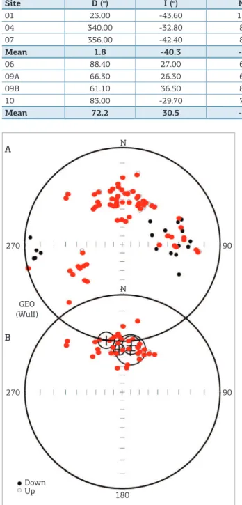
Table 2. Mean magnetization direction, represented by the inclination (I) and declination (D), sample numbers for each site (N) and statistical parameters R, K and α
95 (
o), as described in the text.
Site D (o) I (o) N R K α
95 ( o)
01 23.00 -43.60 10 9.9 140.4 8.30
04 340.00 -32.80 8 7.9 155.4 5.70
07 356.00 -42.40 8 7.8 42.1 5.50
Mean 1.8 -40.3 -- -- -- 17.6
06 88.40 27.00 6 5.9 36.5 9.60
09A 66.30 26.30 6 5.8 24.4 21.20
09B 61.10 36.50 8 7.7 25.3 10.80
10 83.00 -29.70 7 6.9 79.9 11.20
Mean 72.2 30.5 -- -- -- 21.2
N
N
180
90 270
90 270
A
B GEO (Wulf)
Down Up
Figure 8. Stereographical projection of mean directions of all sites of GAP (A) and of the sites that presents coherent magnetizations directions with acceptable statistical parameters (sites 1, 4 and 7) (B). Open circles for upper hemisphere and solid circles for lower hemisphere.
MAG3D, 2002). he algorithm assumes that the source region is represented by a set of rectangular cells in a 3D orthogonal mesh with magnetic susceptibility (κ) constant in each cell. Since the number of cells is grater than the number of available data, as pointed out by Li and Oldenburg (1996), they proposed the introduction of an objective function
that can incorporate a priori information, with appropriate weighting that is minimized and can produce a geological acceptable model. his objective function is described as (Li & Oldenburg 1996):
(
)
∫
V s sm =α W wz dV+
φ 2
2 ] )[ ( )
(
∫
∂ ∂
V x
x dV+
x z w W
α ( )
∫
V y ∂ ∂y dV+
y z w W
α ( )
∫
∂ ∂
V z
z dV
z z w W
α ( )
K,K→0 K -K→ →0
] [ K -K→ →0
2 ] [ K -K→ →0
2 ] [ K -K→ →0 →
⎞ ⎟ ⎟ ⎠ ⎞
⎟ ⎟ ⎠
⎞ ⎟ ⎟ ⎠ ⎞
⎟ ⎟ ⎠
⎞ ⎟ ⎟ ⎠ ⎞
⎟ ⎟ ⎠
(2)
In the objective function of model the terms Ws, Wx,
Wye Wzare spatially dependent weighting functions and αs,αx, αy and αz are coeicients that afect the relative importance of diferent components in the objective func-tion. he weight function w(z) does not allow that mag-netic susceptibility be concentrated near the surface. It is convenient to write Eq (2) as φm(p) = φms + φmv where φms refers to the irst term in Equation (2) and φmv refers collectively to the three remaining terms involving the variation of the model in the three spatial directions. he reference model can be included in φms and if necessary, remove any remaining other terms.
Li and Oldenburg (1996) used a weight function w
to prevent the rapid decay of magnetic surface data with depth in the resolution. If this fact is not controlled the magnetic susceptibility is concentrated near the surface. he weight function, w(z) = (z−z0)−β/2, is then applied into φ
ms
and optionally into φmv, β is usually set equal to 3 and z0
depends on the cell size of the model and the altitude of the observation data. he steps for discretization of the model are described in Li and Oldenburg (1996).
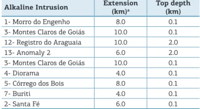
Table 3. Initial parameters for the reference model in the 3D magnetic inversion.
Alkaline Intrusion Extension
(km)a
Top depth (km)
1- Morro do Engenho 8.0 0.1
3- Montes Claros de Goiás 10.0 0.1
12- Registro do Araguaia 10.0 2.0
13- Anomaly 2 6.0 2.0
3- Montes Claros de Goiás 10.0 0.1
4- Diorama 4.0 0.1
5- Córrego dos Bois 8.0 0.1
7- Buriti 4.0 0.1
2- Santa Fé 6.0 0.1
aX and Y extension have the same value. values positives. his is achieved by minimizing φ = φd +
λφm subject to κj > 0, as shown in Equation (3):
( )
ln
+
W λ
+
d d W
=
φ M
j= m
calc obs
d –
1 2 2
2ζ
) (
)
( K – K→ →0 ∑ Kj (3)
where φ is the global objective function, λ is the regulariza-tion parameter and ζ is the barrier parameter for the max-imum and minmax-imum values of the magnetic susceptibility contrast. In Equation (3), λ controls the relative importance of the model norm and data itting. he constraint of pos-itivity is implemented in the logarithmic term of Equation (3) (Li & Oldenburg, 2003).
he presence of strong remnant magnetization can pose severe challenges to the quantitative interpretation of magnetic data. Problems stem from the fact that the direction of total magnetization is unknown and can be signiicantly diferent from that of the current induc-ing ield. In applications such as crustal scale studies the remanence is often very strong and cannot be ignored. Inversion techniques require recovered causative bodies to reproduce the observed data, and this dictates that we must know the magnetization direction. Unrealistic distribution of magnetization and susceptibilities can result from inversion if incorrect direction is speciied. Faced with this diiculty, one can take several diferent approaches. he irst is to physically measure the rem-nant magnetization by oriented sample, with number of samples may necessarily give good characterization of the bulk magnetization direction. Once you have the knowledge of the direction of the remnant magnetization taken from oriented samples, we can use the total mag-netization direction as the vector sum of the directions of magnetization induced more remaining.
We present a method for inverting surface magnetic data to recover 3-D susceptibility models. To allow the maximum lexibility for the model to represent geologically realistic structures, we discretize the 3-D model region into a set of rectangular cells, each having a constant susceptibility. he number of cells is generally far greater than the num-ber of the data available, and thus we solve an underdeter-mined problem. Solutions are obtained by minimizing a global objective function composed of the model objective function and data misit. he algorithm can incorporate a priori information into the model objective function by using one or more appropriate weighting functions. How the algorithm assumes that there is no remnant magnetiza-tion and that the magnetic data are produced by induced magnetization only, we can use the total magnetic inten-sity and direction of the total magnetization as the vec-tor sum of the directions of magnetization induced more magnetization remnant.
RESULTS OF MAGNETIC INVERSION
he study area was divided into a set of cubic cells with 2 km side and constant value for the magnetic suscepti-bility. he initial model is composed of prisms centered in the anomaly positions outlined in Fig. 8, with the top at the surface, 0 km, and the base at 12 km depth.
he MAG3D inversion algorithm (MAG3D 2002) uses only induced magnetization, but the GAP alkaline intru-sions have a strong remnant component as it was discussed previously. To overcome this situation it was used the direc-tion of the total magnetizadirec-tion of the main alkaline sources. It was considered only the specimens that showed consistent magnetization directions to determine the average direction of the remnant magnetization so it was only considered sites 01, 04 and 07, as shown in Fig. 7B. he value obtained for the mean direction of remnant magnetization was IR = -40.3º and DR = 1.8º. he vector sum of the components of the induced magnetization MI (magnetic ield at the time of survey in the area has I = -19.5° and D = -18.5 °) and rem-nant magnetization MR resulted in the direction of the total magnetization used in the inversion procedure, IT = -39.0º and = DT = 1.0 º.
Results from magnetic susceptibility measurements on the samples were set as the initial values of magnetic suscep-tibility (κ) in model, with κ varying according to values of Fig. 2. he values for the lateral extension of the intrusions were obtained by the analysis of the map of GHT and ASP (Fig. 8). Depth of the top was set at 0 km for the outcrops and 2 km for the two magnetic anomalies with no geologi-cal evidence on the surface. Geometrigeologi-cal parameters for the initial model are summarized in Table 3.
cells in x and y directions than the reference model used. For most of the GAP intrusions the depth was around 10 – 12 km, except Registro do Araguaia with magnetic susceptibility at depths up to 16 km. he possible intrusion that corresponds to this anomaly (n. 12) does not outcrop. Its top depth was estimated by Dutra et al. (2012) from the Euler deconvolution method combined with analytical signal amplitude applied to the magnetic anomaly reduced to the pole. Dutra et al. (2012) found the top at a depth around 600 – 800 meters. Figure 9 shows slices of mag-netic susceptibility variation at depths varying from 2 to 16 km. he subsurface distribution is not homogeneous with depth; most of the intrusion has more area with phys-ical property contrast at 6 – 8 km depth. Another feature is the dispersion of susceptibility at depth in the south part the area, especially at the depth of 12 – 14 km, suggesting a smooth connection among them. his distribution allows a hypothesis of some intrusions with more spherical shapes than cylinder, as could be expected for alkaline intrusions that usually resembles pipe structures.
From the distribution model (Fig. 9) it was calculated the magnetic ield by forward modeling and its result was com-pared with the observations as can be seen in Fig. 10. he mod-eled magnetic amplitude its the data, but the magnetic ield (red line) is smoother compared with observation (black line).
100
80
60
40
20
100
80
60
40
20
100
80
60
40
20
100
80
60
40
20
100
80
60
40
20
100
80
60
40
20
(km)
(km)
Z=1 – 2 km Z=2 – 4 km Z=6 – 8 km
Z=10 – 12 km Z=12 – 14 km Z=16 – 18 km
20 40 60 80 20 40 60 80 20 40 60 80
20 40 60 80 20 40 60 80 20 40 60 80
(km) (km) (km)
(SI) 0.1 0.09 0.08 0.07 0.06 0.05 0.04 0.03 0.02 0.01 0
Figure 9. Magnetic susceptibility distribution in depth from the 3D inversion. Slices cut at diferent depths.
Figure 10. Total ield magnetic anomaly (black line) and magnetic anomaly calculated from the inversion magnetic susceptibility distribution (red line).
Total field magnetic anomaly observed and calculated
110
100
90
80
70
60
50
40
30
20
10
0
0 10 20 30 40 50 60 70 80
0 5 10 15 20
(km)
Observed
his smoothing results from the limited number of cells that the program allows and combined with the choice of invert-ing all the area together instead of diferent groups of anom-alies. his choice relects the main focus of this work that is to understand the emplacement of the intrusions within the crust, which resulted in the maximum possible number of cells with a larger size.
The results in Fig. 10 represent the contribution of the magnetic ield produced by the remnant magnetiza-tion more induced magnetizamagnetiza-tion used as the ”induced magnetic ield” as a work hypothesis. his is not the strict way for the MAG3D inversion algorithm but the good it between observation and model indicates that the chosen way worked adequately.
DISCUSSION AND CONCLUSIONS
he aeromagnetic signal of the alkaline intrusions of the GAP was used to obtain the magnetic susceptibility tion in subsurface and the model may represent the distribu-tion of magnetic mineral content. he authors knew from previous work (Dutra & Marangoni 2009) that the mag-netic signal observed in the area is a combination of induced and remnant magnetic components. he diicult to invert a source with remnant magnetism is great and this resulted in a search for a diferent path using known algorithm. he path chosen was to use the sum vector of the components as the induced ield in the area. To accomplish this proce-dure a careful analysis of remnant component was done.
he main component of remnant magnetization was iso-lated using alternate magnetic ield and thermal demagneti-zation. he results considering just the most stable samples and with acceptable statistical parameters, sites 01, 04 and 07 as is seen in Table 2, resulted in remnant inclination and declination of -40.3o and 1.8o, respectively. hese
val-ues were summed with the induced ield at the light time to provide values for the inversion algorithm. Measurements of magnetic susceptibility and density also provided values for physical parameter in the inversion.
To complete the initial model the geometry of the sources was preliminary ind with the application of Total Horizontal Gradient and Analytical Signal Phase on the total anomaly ield reduced to the pole. he superimposed map with the two results (Fig. 8) marks the contact lim-its and also some NW-SE faults that cross the anomalies without changing their shape. his may suggest that this faults or lineaments were weakness regions and the alka-line magma may take advantage of it during the emplace-ment. he NE-SW lineaments in the north of Registro do Araguaia (anomaly 12 in Fig. 8) may be a diferent case.
We propose that this anomaly is located at the southern end of the Transbrasiliano Lineament and that the magma emplacement illed the fractures of the lineament. We also propose that Registro do Araguaia and its NE-SW linea-ment may be the main locus for magma conduit based on the anomaly size, strong magnetic expression and source size from inversion. he two main direction observed in Fig. 8 were reactivated as extensional tectonics during magma ascent. he NW-SE lineament, with traces in the magnetic maps, was very active and in this direction it is possible to ind other alkaline provinces, the Alto Paranaíba Province (APIP), at the SE of the area and Poxoreu Province at the NW of the area. A discussion of the importance of this lin-eament can be found in Marangoni and Mantovani (2013).
he results from the 3D inversion indicate that the intru-sions extents through the upper crust, from surface up to 10 – 12 km. he results suggest that the shapes of the bod-ies are conical. Except for the Registro do Araguaia shows diferences respecting the other intrusions. Its depth goes up to 16 km and the area involved is also bigger than the rest of the intrusions. It is reasonable to consider that Registro do Araguaia is one of the most important magma feeder for the GAP intrusions. By the 3D inversion, the magnetic sus-ceptibility is distributed in almost spherical and cylindrical shapes. he possibility of spherical shapes arise the hypothe-sis that the GAP intrusions at the north part of the province represent magmatic chambers. he alkaline magma ascend from the lithosphere, used the two main fault systems as space for emplacement. Results from magnetic inversion conirm the conclusions from Junqueira-Brod et al. (2005) and Dutra et al. (2012).
isotopic compositions similar to the Paraná lood basalts, the results presented here suggest that the Paraná high-Ti source, and that of the isotopically similar oceanic basalts of the Walvis Ridge, formed in the Brazilian lithosphere in the Proterozoic.
Acknowledgments
his work was supported by Fundação de Amparo à Pesquisa do Estado de São Paulo – FAPESP, 2006/00201-2 and 2007/53179-7. he authors acknowledge M. B. Lacerda for density measurements.
Blakely R.S. 1996. Potential theory in gravity and magnetic applications. Cambridge, Cambridge University Press.
Books G.K. 1962. Remanent magnetization as a contributor to some
aeromagnetic anomalies. Geophysics, 27(3):359-75.
Brod J.A., Barbosa E.S.R., Junquieira-Brod T.C., Gaspar J.C., Diniz-Pinto
H.S., Sgarbi P.B.A., et al. 2005. The Late Cretaceous Goiás alkaline
Province (GAP)m Central Brazil. In: Comin-Chiaramonti, P. & Gomes, C.B. (eds.). Mesozoic to Cenozoic alkaline magmatism in the Brazilian platform. São Paulo; EDUSP-FAPESP. pp. 261-416.
Carlson R.W., Araujo A.L.N., Junqueira-Brod T. C., Gaspar J.C., Brod J.A., Petrinovic I.A., et al. 2007. Chemical and isotopic relationships
between peridotite xenoliths and maic– ultrapotassic rocks from
Southern Brazil. Chemical Geology, 242(3-4):415-34.
Comin-Chiaramonti P. & Gomes C.B. (eds). 2005. Mesozoic to Cenozoic alkaline magmatism in the Brazilian platform. São Paulo; EDUSP-FAPESP, 752p.
Cox K.G., Bell J.D., Pankhurst R.J. 1979. The interpretation of igneous rocks. G. London; Allen & Unwin.
Dutra A.C., Marangoni Y.R. 2009. Gravity and magnetic 3-D inversion
of Morro do Engenho complex, central Brazil. Journal of South
American Earth Sciences, 28(2):193-203.
Dutra A.C., Marangoni Y.R., Junqueira-Brod T.C. 2012. Investigation of the Goiás Alkaline Province, Central Brazil: Application of gravity
and magnetic methods. Journal of South American Earth Sciences,
33(1):43-55.
Fisher R. 1953. Dispersion on a sphere. Proceedings of the Royal
Society of London - Series A, 217:295-305.
Junqueira-Brod T.C., Riog H.L., Gaspar J.C., Broad J.A., Meneses P.R. 2002. A Província Alcalina de Goiás e a extensão de seu vulcanismo kamafugítico. Revista Brasileira de Geociências, 32(4):559-66.
Junqueira-Brod T.C., Gaspar J.C., Brod J.A., Jost H., Barbosa E.S.R.,
Kaino C.V. 2005. Emplacement of kamafugite lavas from the Goiás
Alkaline Province, Brazil: constraints from whole-rock simulations. Journal of South American Earth Sciences, 18(3-4):323-35.
Lacerda Filho J.V., Rezende A., Silva A. 2000. Programa Levantamentos
Geológicos Básicos do Brasi. Geologia e Recursos Minerais do Estado de Goiásb e do Distrito Federal. Escala 1:500000 (mapa) 2ª Edição. CPRM/METAGO/UnB. 184 pp.
REFERENCES
LASA Engenharia e Prospecções S.A. 2004. Projeto Levantamento Aerogeofísico do Estado de Goiás – 1ªEtapa – Arco Magmático de
Arenópolis – Complexo Anápolis - Itauçu – Sequência
Vulcano-Sedimentar de Juscelândia. Relatório Final do Levantamento e Processamento dos Dados Magnetométricos e Gamaespectrométricos, Convênio de Cooperação Técnica entre a SGM/MME/CPRM e SIC/ SGM/FUNMINERAL/Estado de Goiás, Relatório Final, 22 vol., Texto e Anexos (mapas), Rio de Janeiro.
Le Bas M.J., Le Maitre R.W., Streckeisen A. Zanettin B. 1986. A
chemical classiication of volcanic rocks based on the total
alkali-silica diagram. Journal of Petrology, 27(3):745-750.
Le Maitre R.W. 1989. A classiication of igneous rocks and glossary of terms. Oxford: Blackwell Scientiic Publications. 193p.
Li Y., Oldenburg D.W. 2003. Fast inversion of large-scale magnetic data using wavelet transforms and a logarithmic barrier method. Geophysics Journal International, 152(2):251-65.
Li Y., Oldenburg D.W. 1996. 3D inversion of magnetic data. Geophysics, 61(2):394-408.
MAG3D. 2002. A program library for forward modeling and inversion of magnetic data over 3D structures, version 3.1,
Department of Earth and Ocean Sciences. Vancouver; University
British Columbia.
Marangoni Y.R., Mantovani M.S.M. 2013. Geophysical signature of
alkaline intrusions bordering the Paraná Basin. Journal of South
American Earth Science, 41:83-98.
Reid A.B. 1980. Aeromagnetic survey design. Geophysics. 45(5):973-6.
Roest W. R., Pilkington M. 1993. Identifying remnant magnetization
efects in magnetic data. Geophysics, 58(5):653-9.
Sgarbi P.B.A., Clayton R.N., Toshiko KM., Gaspar J.C. 1998. Oxygen isotope thermometry of Brazilian potassic volcanic rocks of
kamafugitic ainities. Chemical Geology, 146(3):115-26.
Tauxe L. 2002. Paleomagnetic principles and pratice. Kluwer Academic Publishers, Dordrecht.
Telford W.M., Geldart L.P., Sherif R.E. 1990. Applied Geophysics. New
York, Cambridge University Press.