Escola de Engenharia
Luís Diogo Monteiro Duarte Couto
Analysing call graphs for software
architecture quality profiling
Dissertação de Mestrado
Escola de Engenharia
Departamento de Informática
Luís Diogo Monteiro Duarte Couto
Analysing call graphs for software
architecture quality profiling
Mestrado em Engenharia Informática
Trabalho realizado sob orientação de
Professor José Nuno Oliveira!
This dissertation could not have been written without the help of several fine people. In no particular order, I would like to thank:
• José Nuno Oliveira for supervising this project. His guidance and encouragement were invaluable.
• Manuel Alcino Cunha for first getting me interested in Formal Methods which eventually led to this dissertation.
• Joost Visser and SIG for the opportunity to work on this project, for assistance and suggestions on many issues and for supporting me financially on a conference trip.
• Eric Bouwers for graciously allowing the use of the IIOT model and assistance with the model analysis process.
• Miguel Ferreira for countless suggestions and constant assistance and advice on the project.
• Tiago Veloso for assistance with formatting and templates. • A personal thanks to my family for their patience and support.
Software has become ubiquitous in today’s world. It is therefore obvious that software quality has become a chief concern of researchers and practitioners alike. Nowadays, Software Architecture is a core dimension of software quality. With the continuous increase in the size of software systems, its importance has grown further and further.
A good way to tackle quality from an architectural point of view is by focusing on com-plexity. Complexity is a primary reason for failure in software systems. We are particularly interested in a metric for complexity. One that is mathematically based and fundamentally sound. We present such a metric.
As software systems have grown in size and complexity, models have emerged as an excellent to way to analyse and reason about the architecture of a system. We present two architectural models: IIOT, which is focused on the organisation and structure of source code files and the connections between them; and SIP, which is focused on the higher level structure and functionalities of the software system.
This dissertation analyses and combines the two architectural models. We present a single unified model. This model has also been enriched with a metric for complexity. We also present a prototype tool that extracts architectural information from a software system’s call graphs, builds the unified model for the system and calculates its complexity.
Furthermore, we perform an extensive analysis of the complexity metric by conducting tests on a large variety of software systems. We also explore the possibility of deriving functionality directly from a call graph via the application of clustering techniques.
O software está em todo o lado nos dias de hoje. Por isso, é óbvio que a sua qualidade se tenha tornado numa grande preocupação quer para investigadores quer para praticantes. A arquitectura de software é hoje uma dimensão chave para a qualidade de software. Com o aumento constante do tamanho dos sistemas, a importância da sua arquitectura só tem aumentado.
Uma boa maneira de atacar a questão da qualidade dum ponto de vista arquitectural é concentrando-nos na complexidade. A complexidade é uma das principais causas de falhas em sistemas de software. Há pois todo o interesse em desenvolver métricas para complexidade bem fundamentadas na matemática. Iremos apresentar tal métrica.
À medida que as arquitecturas de software têm aumentado em tamanho e complexidade, os modelos emergiram como um bom modo de analisar e raciocinar sobre a arquitectura dum sistema. São apresentados dois modelos arquitecturais: IIOT que está focado na organização e estruturação dos ficheiros de código fonte e nas conexões entre eles; e SIP que está focado na estrutura alto-nível e ligações das funcionalidades do sistema.
Esta dissertação analisa e combina esses dois modelos arquitecturais num único modelo unificado que é enriquecido com uma métrica de complexidade arquitectural. Apresenta-se também uma ferramenta protótipo que extrai a informação arquitectural do grafo de invo-cação (“call graph”) do sistema de software e que constrói o modelo unificado respectivo e calcula a complexidade do sistema de acordo com a métrica.
A métrica de complexidade arquitectural proposta é analisada extensivamente, através de testes e medições realizadas em vários sistemas de software. É também explorada a possibilidade de derivar as funcionalidades de um sistema directamente a partir do seu “call graph” com a aplicação de técnicas de classificação (“clustering”).
Contents iii
List of Figures vi
List of Tables vii
List of Listings ix
Acronyms xi
1 Introduction 1
1.1 Basic Motivation . . . 1
1.2 Software Archicture Evaluation . . . 2
1.3 Architectural Information . . . 3
1.4 Aims . . . 3
1.4.1 Clustering . . . 5
1.4.2 Quality Metric . . . 5
1.5 Background Information . . . 6
1.5.1 Introducing Call Graphs . . . 6
1.5.2 Introducing Alloy . . . 7
1.6 Structure . . . 8
2 Software Architecture State of the Art Review 11 2.1 A brief history . . . 11
2.2 Fields of software architecture research . . . 13
2.2.1 Software Architecture Evaluation . . . 13
2.2.2 Architecture Description Languages . . . 15
2.4 Challenges . . . 22
2.5 Summary . . . 23
3 Two Architectural Metamodels 25 3.1 IIOT Model . . . 25 3.1.1 Model Description . . . 25 3.1.2 Alloy Analysis . . . 26 3.1.3 Discussion . . . 27 3.2 SIP Model . . . 30 3.2.1 Model Description . . . 31 3.2.2 Alloy Analysis . . . 32 3.2.3 Discussion . . . 34 3.3 Unification . . . 34 3.4 Summary . . . 36
4 From Methods to Functional Groups 39 4.1 Early Approaches . . . 39
4.2 Mathematical Approaches . . . 41
4.3 Clustering Techniques . . . 41
4.4 Final Remarks . . . 45
5 Applying the SIP Metric to IIOT Models 47 5.1 A Formula for Complexity . . . 47
5.2 Discussing the Metric . . . 48
5.3 IIOTool Functionalities . . . 51
5.4 Working with Call Graphs . . . 51
5.5 Prototype Development Notes . . . 54
5.6 Usage . . . 55
5.7 Future Improvements . . . 57
5.8 Summary . . . 58
6 Studying Architectural Complexity 59 6.1 Preparation Work . . . 59
6.2 Questions and Hypotheses . . . 60
6.3 Running the Tests . . . 61
6.4.1 Statistics on Metrics . . . 61
6.4.2 Analysis . . . 62
6.4.3 Correlations on multiple systems . . . 64
6.4.4 Analysis . . . 66
6.5 Results for two systems across time . . . 68
6.5.1 Statistics on Metrics . . . 69
6.5.2 Analysis . . . 69
6.5.3 Correlations across snapshots . . . 72
6.5.4 Analysis . . . 73 6.6 Summary . . . 75 7 Conclusion 77 7.1 Overall Review . . . 77 7.2 Metric assessment . . . 78 7.3 Future Work . . . 80 Bibliography 83 Index of Terms 91 A Alloy Models 95 A.1 IIOT Model . . . 95
A.2 SIP Model . . . 99
B Features versus Clusters 105 C Case Studies Data 109 C.1 Histograms . . . 110
C.2 Correlations . . . 115
C.3 Plots . . . 115
C.3.1 System A . . . 115
1.1 A (very) simple callgraph example. . . 6
2.1 Example concept lattice . . . 18
2.2 Concept lattice with citation keys and attributes . . . 19
2.3 Concept lattice with extent object counts . . . 20
3.1 Alloy metamodel for the IIOT model. . . 27
3.2 Alloy metamodel for SIP model. . . 33
3.3 IIOT and SIP metamodels side by side. . . 35
3.4 IIOT and SIP metamodels side by side w/ hidden elements. . . 36
3.5 Unified SIP and IIOT model . . . 37
4.1 Cropped method call graph of our test case system. . . 40
4.2 A weakly connected graph. . . 42
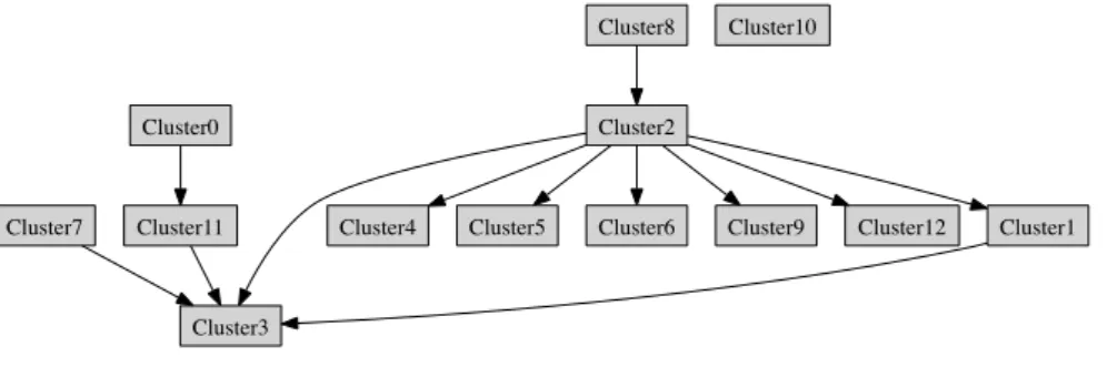
4.3 The clustered graph produced by the edge betweenness algorithm. . . 43
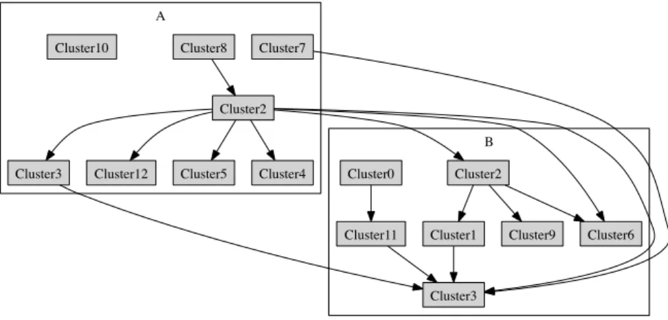
4.4 Clustered graph with components. . . 44
5.1 A system with two components and one connection. . . 49
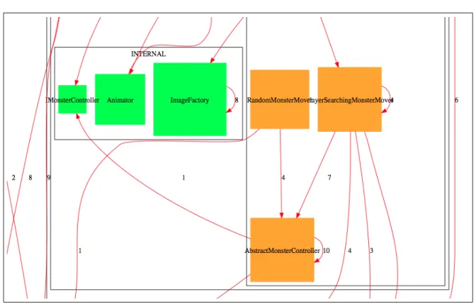
5.2 Crop of an example IIOT model constructed with DOT. . . 55
6.1 Volume distribution across multiple systems. . . 62
6.2 Architectural complexity distribution across multiple systems. . . 63
6.3 Q-Q plot for architectural complexity distribution across multiple systems. . . . 65
6.4 Various metrics plotted across snapshots of system A. . . 71
6.5 Various metrics plotted across snapshots of system B. . . 72
B.2 Methods grouped by clusters and coloured by feature group. Methods w/o
feature removed. . . 107
C.1 CB distribution across multiple systems . . . 110
C.2 Dependency count distribution across multiple systems . . . 111
C.3 Component count distribution across multiple systems . . . 112
C.4 Volume distribution across multiple systems . . . 113
C.5 Volume distribution across multiple systems (finer-grained) . . . 114
C.6 Volume plot for system A . . . 115
C.7 Complexity plot for system A . . . 116
C.8 Component and dependency count plots for system A . . . 116
C.9 Component balance plot for system A . . . 117
C.10 Combined metric plot for system A . . . 117
C.11 Volume plot for system B . . . 118
C.12 Complexity plot for system B . . . 118
C.13 Component and dependency count plots for system B . . . 119
C.14 Component balance plot for system B . . . 119
2.1 Example of object and attribute matrix. . . 17
5.1 An excerpt of a call graph in CSV form. . . 52
5.2 An excerpt of component information in CSV form. . . 52
5.3 An excerpt of file size information in CSV form. . . 52
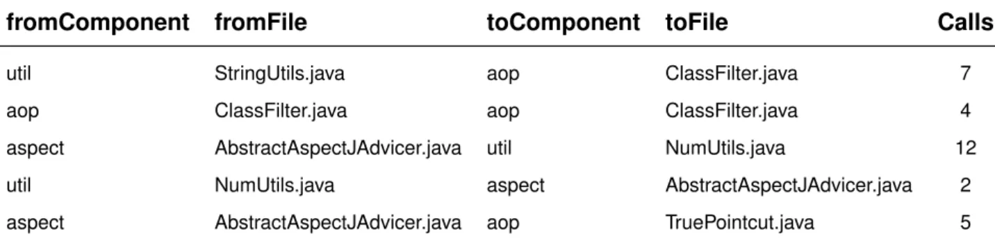
5.4 A few rows from a data warehouse storing method, class and component call information. . . 53
6.1 Statistical analysis for metrics across multiple systems . . . 62
6.2 Normality tests for architectural complexity distribution across multiple systems 64 6.3 Metric correlations across multiple systems . . . 66
6.4 Stratified correlations between volume and complexity . . . 68
6.5 Statistical analysis for metrics across multiple snapshots of system A . . . 69
6.6 Statistical analysis for metrics across multiple snapshots of system B . . . 69
6.7 Metric correlations across multiple snapshots of system A . . . 73
6.8 Metric correlations across multiple snapshots of system B . . . 73
C.1 Stratified correlations between component count and complexity . . . 115
1.1 A relation in declared in Alloy. . . 7
1.2 Multiple relations declared in Alloy. . . 8
1.3 Simple predicate in Alloy. . . 8
1.4 Checking an assertion in Alloy. . . 8
3.1 Alloy model for IIOT. . . 26
3.2 General call rules for the IIOT Alloy model . . . 28
3.3 Module type call rules for the IIOT Alloy model . . . 29
3.4 Alloy model for SIP. . . 32
3.5 Rule for component connections in the SIP Alloy model . . . 33
A.1 Complete Alloy model for IIOT. . . 99
AADL Architecture Analysis & Design Language. ADL Architecture description language.
ATAM Architecture Tradeoff Analysis Method. CB Component balance.
CSV Comma-separated values.
API Application programming interface.
IIOT Internal, Incoming, Outgoing and Throughput. SIG Software Improvement Group.
LiSCIA Lightweight Sanity Check for Implemented Architectures. LoC Lines of code.
OLAP Online analytical processing. OO Object-oriented.
SA Software architecture.
SAAM Software Architecture Analysis Method. SAR Software architecture reconstruction. SIP Simple Iterative Partitions.
SOA Service-oriented architecture. UML Unified Modeling Language.
Introduction
1.1
Basic Motivation
Software has become such a crucial part of our lives that we depend on it in many ways (shopping, healthcare, banking, transportation, etc...). It therefore stands to reason that we are all interested that the software we use or develop is the best possible [20].
So we arrive at the first important notion in this dissertation, software quality, which has become a major concern in today’s software community [38]. Quality means much more than simply writing good source code, it must be a part of the entire software process[33].
There are many facets and angles to software quality. These range from performance and “absence of bugs” to how easy it is to change the software (modifiability) or test it (testa-bility). These different aspects of software quality are called software quality attributes.
There are, of course, many other aspects that are also relevant to the quality of a software system, including the quality of the source code itself. The software architecture (SA) of a system is a very strong factor for quality[6] because it “allow[s] or preclude[s] nearly all of the systems quality attributes” [19].
SA can be defined as “the structure or structures of the system, which comprise software components, the externally visible properties of those components, and the relationships among them.” [6].
It is also important to mention the measuring of software quality. As previously stated, software quality is reflected in a series of quality attributes. In order to measure the quality of a software system, we must establish the desired quality attributes and measure them. In order to measure a quality attribute we need metrics. The ones we use are usually called software quality metrics. It should be noted that not all quality attributes can be measured
directly. For example, the only way to directly evaluate the maintainability of a software system is to evaluate the time and resources spent by developers doing maintenance and not by measuring any metric on the system itself. However, it is possible to use metrics as predictors for certain given quality attributes. These metrics are referred to as metrics by proxy.
Our focus in on how to measure quality from an architectural complexity point of view. Therefore, we need a metric that relates to SA complexity.
1.2
Software Archicture Evaluation
As previously stated, we need a way to evaluate the architectural quality of a system. How good is the architecture? To what extend does (or will) it support the desired quality at-tributes? Clearly, we need metrics (and perhaps quality attributes) that are designed espe-cially for SA.
Furthermore, SA is a fairly abstract concept and there are many models for representing and working with it. Each model tends to have its own focus or specialty. One of the most famous examples is Architecture Analysis & Design Language (AADL)[27] which focuses on embedded systems, software/hardware interactions and correctness.
This dissertation presents two architectural models: Simple Iterative Partitions (SIP) pro-posed by Roger Sessions [60] and Internal, Incoming, Outgoing and Throughput (IIOT) de-veloped by Eric Bouwers et al. [13].
The SIP model puts it that complexity is an important part of architectural quality, though not the only one. SIP follows a principle that, everything else being equal, the less complex a system is, the better. SIP proposes both a model for representing the architecture as well as a metric (and respective formula) to measure the system’s complexity. It is designed to work in the conceptual stages of software development. SIP typically evaluates an architecture in the design stages and its models use the system’s functionalities as major elements. While this is a perfectly valid and useful approach, this dissertation aims to evaluate the architecture of implemented systems. This is where IIOT comes in.
The IIOT model focuses on implemented architectures taking a much more structural view of a system’s SA. In fact, the IIOT model of a given software system can be extracted from its source code, which means we do not need to perform a functional analysis of a sys-tem. IIOT presents the architecture of a system resorting to a system’s modules (generally, the various source code files) and components (sets of modules). IIOT defines a taxonomy
for classification of modules.
Both models have already been developed and validated. The main challenge is to com-bine them into a single, unified model. The idea is to harmonize both models and include them into a single process that, for a given software system, will allow one to reverse-engineer a model for the SA and then measure the quality of that architecture.
1.3
Architectural Information
SA is an abstract concept and therefore only implicitly present in a system. SA models al-low us to visualize architecture although one needs a way to extract it. One must analyse systems and extract architectural information in order to build the models. This dissertation will focus on approaches that use static analysis. This is in line with the standard software evaluation procedure at Software Improvement Group (SIG). Many elements and data ob-tained from a software system could be used for static analysis. We will work exclusively with call graphs and extract architectural information from them. An advantage of using call graphs is that any system and language that features calls (as most do) can have a call graph. Another one is that call graphs contain everything needed to build SA models. This is a powerful abstraction of code that allows one to channel all resources and time into a single area, hopefully leading to more focused results.
Extraction, storage and processing of call graphs are all activities that must be kept in mind. We shall not be concerned with the extraction processes, as SIG has technology for doing so, kindly providing call graphs for experiments. Call graph information is fairly simple so its storage should not be a problem. Because of its simplicity, we look into a few concepts from data warehouses [17] and Online analytical processing (OLAP) [17] when considering storage. Processing the call graphs and using them to construct our models is obviously a very important part of this project.
1.4
Aims
This dissertation evolved from a number of research questions which are listed below, to-gether with associated tasks. The prime objective was to unify two SA models (SIP and IIOT) based on a formal analysis.
Task 1.a: Formal analysis of terminology of the models. Task 1.b: Modeling of a single, intermediate, representation.
The main hope behind the compatibility analysis of both models is to assess the utility of the complexity metric from SIP when used with the IIOT model. This is made implicit in another objective:
Question 1.1: Can we use SIP’s metric with IIOT?
Task 1.1.a: Identify necessary elements for metric usage.
Task 1.1.b: Locate/add key elements for the metric to the IIOT model.
Task 1.1.c: Devise an algorithm for computing the metric with the IIOT model.
Before we can contribute anything to the field of SA, it is important that we gain a good understanding of the field itself and the research that has already been carried out. To-wards that end, a survey of SA literature is carried out in order to answer the three following questions:
Question 2.a: What has been achieved thus far? Question 2.b: What are the recent breakthroughs? Question 2.c Which shortcomings remain?
The SIP model is built on a notion of business functions: independent pieces of function-ality provided by a system. These are used in the complexity calculation for the system. In the SIP model, these business functions are constructed manually (for example, by analysing the design documents). On the other hand, the IIOT model is built automatically from the source code and so there is an interest in examining the relationship between source code and business functions, as shown by the following questions.
Question 3: Is it possible to derive business functions from static call graph analysis? Question 3.a: Does it make sense to reduce the methods in a call graph to method
groups?
Question 3.b: Is it within reach to obtain a “good” reduction?
Question 3.c: Can such analyses be performed in an automated manner on static
It was also decided to place great focus on the complexity metric by performing a detailed analysis of it. This is reflected in the following question and tasks. This was also used to power our case study and served as validation for the metric and related research done throughout the dissertation.
Question 4: What can we learn about the complexity metric when applied to IIOT instances? Task 4.a: Perform a statistic analysis of the metric by itself.
Task 4.b: Analyse and compare the complexity metric with other software system
met-rics.
1.4.1
Clustering
The information presented in call graphs is ideally suited to constructing the IIOT model since both call graphs and IIOT essentially exist at the same abstraction level (implementa-tion). However, the SIP model works with more abstract concepts such as functionalities (or functional groups). One of the ways in which we attempt to unify both models is by trying to extract SIP model elements from a system’s call graph.
We are interested in ways to group the elements of a call graph (typically methods) into higher level elements (functional groups). We explore several approaches including graph theory and also graph clustering techniques.
Particularly interesting graph clustering techniques show up in the field of community detection [22]. We explore the area under the intuition that some of the work might be applicable in our project.
This is the more experimental aspect of our project with a great deal of trial and error and less expectations in terms of results.
1.4.2
Quality Metric
The main goal of this dissertation is to have a way to measure the complexity of a system from an architectural point of view. We extract the architectural information and use it with the IIOT portion of our work. The metric itself comes from the the SIP portion. Once we have combined both models, we are then able to apply the metric directly to a system.
To help with this we develop a prototype tool that implements the fundamental steps of the process: read a call graph, construct the model, compute the metric. With this tool we
NamespaceHandler.init() ConfigBeanDefinitionParser.$constructor() 1 BigBeanDefinitionParser.$constructor() 1 NamespaceHandlerResolver.resolve(java.lang.String) 1
Figure 1.1: A (very) simple callgraph example.
can evaluate our work on several test systems. We are especially interested in seeing how the SIP complexity metric varies across different systems.
The main contribution of this dissertation is therefore a metric-based approach to measur-ing the complexity of a system’s SA. We use a combination of design and post-implementation models and approaches, thus establishing a bridge among these. We also hope to, indirectly, contribute to the clustering of software call graphs.
1.5
Background Information
1.5.1
Introducing Call Graphs
A call graph is a directed graph that represents referential (calling) relationships among the elements of a software system. It is a (relatively) old and very well established concept [58]. In a call graph, the nodes represent an element of the system, traditionally a function or pro-cedure. Each edge in the graph represents a call between a pair of elements. For example, edge (a,b) tells that element a calls element b.
There are two main types of call graph: dynamic and static. A dynamic call graph cor-responds to a specific and particular execution of a program. Each dynamic call graph is constructed by tracking the execution of a given program. A static call graph, on the other hand, is independent of program execution. It contains all possible calls among elements. Static call graphs are usually extracted from the program source code.
A very simple example of a method-level call graph from a Java system can be seen in Figure 1.1 (in truth, only a subgraph of a much larger system).
for this. First, we can extract static graphs directly from source code, without the need for program execution. This stays with the tradition in SIG’s approach to software evaluation, which is based on source code analysis. Secondly, a static call graph has information about the complete system. A dynamic call graph only contains the units and calls of a particular execution and is therefore not adequate for the kind of architectural analysis we want to perform.
Call graphs can be used to represent information at many different abstraction levels of a system and with varying granularity. We can have the traditional function-level call graph although we can also have a graph for calls at class-level, file-level, package-level and so forth. From a practical standpoint, one typically extracts the lowest level graph (function, method, etc.) and then simply rolls up the nodes to reach the higher levels, as in data mining. Call graphs are generic (they simply have generic units and calls) though in this dissertation we work specifically with Java call graphs (with method calls and so forth).
1.5.2
Introducing Alloy
In this section we will briefly introduce Alloy, a modelling language used later on when we analyse IIOT and SIP. Alloy is a modeling language developed at MIT[37]. It is built upon first order logic and relational algebra (Alloy’s lemma is “everything is a relation” ). Its language is declarative and fairly simple.
Alloy has tool support in the form of the Alloy Analyzer which allows for execution and verification of the modules to search for counterexamples to assertions in the model and the consistency of the model itself (whether it can be instantiated or not). When counterexamples are found, the tool displays a diagram of the model for the user to inspect and explore.
In Alloy, relations are declared using the keyword sig (for signature):
Listing 1.1 A relation in declared in Alloy.
sig A { C : B }
This declares a relation C : A → B. Relations can be further defined with regards to multiplicity with keywords such as lone and one. Furthermore, a single sig may hold multiple relations:
Listing 1.2 Multiple relations declared in Alloy. sig F i l e S y s t e m { f i l e s : set File , p a r e n t : f i l e s - > l o n e files , n a m e : f i l e s l o n e - > one N a m e }
Relations can also be manipulated by several operators such as . (composition), & (intersection) and ˜ (converse).
Finally, in order to express the various properties of a model, Alloy has predicates as shown in Listing 1.4.
Listing 1.3 Simple predicate in Alloy.
p r e d h a s P a r e n t [ f : F i l e ] { s o m e f . p a r e n t
}
Predicates can then be used in assertions (assert command) to place constraints upon the model. These assertions can then be checked for a particular scope (number of in-stances of each relation in the model).
Listing 1.4 Checking an assertion in Alloy.
a s s e r t N o O r p h a n s {
all f : F i le | h a s P a r e n t [ f ] }
c h e c k N o O r p h a n s for 3
1.6
Structure
The remainder of this dissertation is structured as follows:
• Chapter 3 contains the analysis and unification of the two architectural models: SIP and IIOT.
• Chapter 4 discusses our experiences and attempts at applying clustering techniques to call graphs.
• Chapter 5 contains a presentation of the architectural complexity metric and a proto-type tool used to help test our work.
• Chapter 6 presents the analysis or our work, by running the proposed metric on a series of test systems.
• Chapter 7 ends the dissertation with some thoughts about the final result and the process itself as well as some possibilities for future work.
Software Architecture State of the Art
Review
Software architecture (SA) has become a full-fledged discipline in recent years [61]. The field has come a long way from its earliest days when it was little more than a set of practices and methodologies for Object-Oriented programming. This chapter surveys research in the field of SA.
This chapter is structured as follows: Section 2.1 gives a historical overview of SA and discusses major breakthroughs that have taken place in the field; Section 2.2 reviews the state of the art in SA research and is the main part of the chapter; Section 2.3 attempts to apply formal concept analysis to produce a structured view of the overall bulk of research in the field; Section 2.4 discusses some of the present and future challenges for the field of SA; Section 2.5 presents concluding remarks and discusses the outcome of this survey.
2.1
A brief history
SA traces its origins back the 80s [61]. Back then several people were already proposing the decomposition of a program in various modules and ways to look at those modules from a higher level of abstraction. At the same time, recurring software structures for particular domains began to appear (for example oscilloscopes [23]).
The term SA began to appear in the literature in the early 90s and became a research field of its own right. Two papers - [32, 56] - are generally credited with establishing the field and settling its name.
OO programming puts a great focus on separation of concerns, encapsulation and structure. Soon people began talking about OO design and developing metrics for measuring the qual-ity of an OO program [18]. These metrics were designed specifically to handle OO systems and measured unique OO aspects.
Soon enough, formalisms appeared for representing OO systems and concepts such as Classes and Methods. Several OO metrics were also formalized (such as cohesion [14] and coupling [15]) and the field began to move towards a focus on measuring a system’s quality by analyzing its architectural aspects.
A major development was the advent of the Architecture Description Language (ADL). Traditionally, architects reasoned about a SA with simple “box and line” diagrams. ADLs go much further than that. They are actual languages supporting formalisms and are used to model and describe SA. ADL research grew tremendously and very soon several different ADLs came to exist, often competing for the same purpose [51].
With better formalisms in place, the evaluation, or analysis, of a SA became the main focus of research in this field. The main idea is to measure an architecture’s ability to deliver on one (or more) specific quality attributes such as reliability, modifiability, etc. Several meth-ods devoted to particular SA evaluations were developed by the community and surveyed in [5, 25].
Lack of tool support, a problem in the earlier days [39] has begun to subside in more recent times. Quite a few evaluation tools exist today, see for example [3].
Most evaluation methods originally focused on the designed architecture since it exists earlier in the development process and the cost of changing should in principle be lower. However, more work has recently been done on implemented architecture evaluation as part of an overall trend of software quality analysis [12].
A particularly elegant concept that eventually took shape was that of a view. A SA can be very complex and affect multiple domains, for example, hardware, source code, protocols and networking. Architects would often try to cram everything into a single, overly complex diagram. The notion of views argues that a single SA can be viewed and analyzed from multiple separate but interconnected and consistent viewpoints. Each can be represented by its own diagram. Particularly influential was the “4+1” view model [42] which proposes four viewpoints on a system: logical, process, physical and development plus a fifth.
Interestingly, the “+1” view, scenarios, became widely adopted in several evaluation meth-ods leading to so-called scenario-based evaluation [5]. This also ties into the popular concept of an use case, as a scenario is an instance of a use case [42].
Clearly, SA has come a long way and is now a proper research field, although still fairly young and with much untapped potential.
2.2
Fields of software architecture research
We now discuss more in depth about some of the current branches of SA research. There are, of course, many different areas of research. We discuss some of the more important ones.
2.2.1
Software Architecture Evaluation
Evaluation is one of the most important areas in the field of SA research. Evaluation, or analysis, of a SA aims to assess its quality or inherent risks [5, 25].
Quality is generally expressed through several quality attributes (such as modifiability, flexibility, maintainability, etc.). Evaluation typically tries to ensure that the required quality attributes are met by the architecture while also identifying potential risks.
Much work has been done on the development of specific methods for evaluating a SA [5, 25]. Most methods advocate that analysis be performed in the earlier stages of a software project. The rationale is that costs of correcting problems are smaller in earlier stages.
As such, these analysis methods can be said to target a designed architecture. They try to predict the quality or risk of the final system through analysis of the SA. Obviously, the degree of precision in these methods can vary.
On the other hand, methods that analyse an implemented architecture also exist. These methods target an architecture post-implementation and most often from the point of view of the source code. These methods have an advantage in the sense that tools can be devel-oped to automate some of their activities (e.g. static code analysis). The main disadvantage is, obviously, that changing something is much more costly at this stage and any problems uncovered will typically be more expensive to correct than if they had been uncovered earlier on.
Nowadays most software systems have a fairly long lifespan and continue to change and evolve through their lifetime. As a system continues to evolve, it can develop several archi-tectural problems such as drift [56, p. 43] (the system’s implementation becomes less and less adherent to the designed architecture); erosion [56, p. 43] (the implementation specifi-cally violates the architecture); or mismatch [29, 30] (various components of the system do
not properly fit together). These problems can also tie into the concept of technical debt [16] - situations where long-term source code quality is sacrificed to achieve a short-term gain in another area. Technical debt and architectural issues quite often go hand in hand.
Methods that focus on implemented architectures can be employed to detect architectural problems and ensure that they are corrected as the system evolves.
To better contribute to the discussion of SA evaluation methods we begin by presenting two important methods in more detail: the first evaluation method to be developed and one of the most popularly used today.
Software Architecture Analysis Method (SAAM) [40]
SAAM was the earliest method developed for SA analysis. SAAM’s main goal is to identify the risk associated with a particular SA. In terms of quality attributes, it mea-sures modifiability. SAAM uses as input requirements documents and an architectural description. This description relies on three views of the SA: functionality, structure and allocation of the former to the latter. SAAM’s primary method of evaluation is based on scenarios that introduce change (hence modifiability). SAAM has since been adapted and modified to evaluate a SA on other criteria such as reuse [46, 52] and complex-ity [44]. Interestingly, SAAM for evolution and reuse [46] is an example of a method that targets an implemented architecture.
Architecture Tradeoff Analysis Method (ATAM) [41]
ATAM was developed under the idea that the quality attributes of a software system interact with each other. For example, performance and modifiability affect each other. As such, a method that analyzes an attribute in the void might not, in fact, give a proper assessment of the system. ATAM can analyze a SA in relation to multiple attributes and identify trade-off points among them. ATAM relies on the “4+1” model to describe archi-tectures. It uses multiple evaluation techniques such as scenarios and also questions and measures. ATAM is regarded as a well validated and comprehensive method [5].
Several other methods exist such as Architecture-Level Modifiability Analysis (ALMA) [9], Performance Assessment of Software Architectures (PASA) [65], Software Architecture Re-liability Analysis Approach (SARAH) [63], Scenario-based Software Architecture Reengi-neering [8] and Simple Iterative Partitions (SIP) [59]. All these methods vary in goals and applicability. Many of them have reached solid levels of maturity [5]. However, according to a recent survey [4] adoption of these methods is still very low at the industry level, with some exceptions. SIP, for example is used by a consulting firm.
Reference [36] surveys methods for reliability and availability prediction at the SA level, two crucial quality attributes in today’s software systems. They find that no single method is sufficient for predicting reliability and availability. Among the main shortcomings found are lack of tool support and poor validation of the methods.
One final method worth mentioning is Lightweight Sanity Check for Implemented Archi-tectures (LiSCIA) [12]. One of LiSCIA’s strengths is ease of use as it is designed to be usable out-of-the-box. LiSCIA targets implemented architectures and is aimed at preventing architectural erosion.
Additional research into utilizing SA to support quality attributes has also been carried out. For exemple, in [7] the authors investigate how SA can affect usability. They argue that traditional methods for achieving high usability focus almost exclusively on the UI. However, they argue that many usability aspects (for example, the undo functionality) require support from the architecture. They present several usability scenarios that require architectural support and also an architectural pattern that satisfies the scenario. In the end, they conclude that a strong link exists between SA and usability.
Research that directly targets quality attributes is also underway, for instance, work on the relationship between service-oriented-architecture (SOA) and different quality attributes, in particular on how SOA affects each of these attributes [54].
Another interesting area of research related to SA evaluation is software architecture reconstruction (SAR) [26]. These techniques attempt to rebuild a system’s architecture in the context of maintenance tasks. Since the architecture is not explicitly present in the system and evolves over time, it is important to rebuild it in order to analyze it.
2.2.2
Architecture Description Languages
Almost any activity related to SA some way to define and work with the architecture. Origi-nally, this was done in an ad hoc manner with “box and line” diagrams. These days, ADLs are commonly used in many software projects. They are particularly useful in the design phase. We shall begin by presenting two radically different ADLs.
AADL [27]
Originally known as Avionics Architecture Description Language, it was created for modeling software systems in the aviation field. It has an obvious focus on embedded systems though it can be utilized in other contexts. AADL allows one to model both the software and hardware portions of a system. An AADL model can be used as
de-sign reference, to support architecture evaluation and even allows for code generation. AADL is a formal language with a precise semantics. It is typically used for developing critical systems.
Unified Modeling Language (UML) [28]
UML has emerged as the de facto standard for SA modeling and has wide industrial adoption, in spite of being far from universally acclaimed [61]. Its strengths are excel-lent tool support, ease of usage (at least compared to something like AADL) and a fair amount of flexibility. Its weaknesses are a direct consequence of its strengths. UML is not a formal language and its diagrams are always liable to subjective interpretation. This can complicate matters when one of its purposes is precisely to communicate information. In fact, the different ways in which UML can be used is a source of prob-lems [43, 53].
It can be argued that UML and AADL are at opposite ends of the ADL spectrum. One is strictly formal and requires a significant commitment from practitioners in order to be suc-cessfully used in a project. The other is strict at best although it can be utilised in a project with great ease (and clearly, using some ADL support when dealing with the architecture is better than using none). Most ADLs tend to lie somewhere along this spectrum, though the ones surveyed tend to lean more on the AADL side.
Many ADLs also exist with a specific focus on some particular area, as is the case of Wright [2] which focuses on interaction and connection between components and has con-nectors as first class citizens; Rapide [45] which focuses on concurrency, synchronization, events and uses partially ordered event sets as an underlying formalism; or Darwin [48] which focuses on distributed systems.
Several other ADLs exist [51], with varying purposes, tool support and so forth.
One final ADL worthy of note is Acme [31]. Acme is a generic ADL which is frequently used to act as an intermediate format between other ADLs.
2.3
Formal Concept Analysis
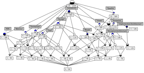
In this section we apply formal concept analysis to SA scientific literature. The idea is to get a more structured overview of the research and maybe draw some interesting conclusions. Also, this can be thought of as an experiment into using concept analysis in the context of
literature organization. This approach has been expanded and led to a paper [21] presented at a conference.
To begin with, a very simple explanation of concept analysis will be given (better intro-ductions to the topic exist elsewhere [66, 57]). Formal concept analysis is a way of automat-ically deriving an ontology from a set of objects and their properties (attributes). Generally speaking, from a matrix of objects and their attributes, one derives relations between sets of objects and the sets of their shared attributes. There is a one-to-one relation between each set of objects and each set of shared attributes. The pairs in this relation are called concepts. There are three types of concept: object and attribute; object only; attribute only.
A set of concepts obeys the mathematical definition of a lattice and can thus be called the concept lattice. This becomes particularly useful in terms of visualising information. An
Object Attribute
Book1 Free
Book1 Hard Copy Book2 Digital Version Book2 Hard Copy Book4 Digital Version Book5 Available from Library
Book5 Free
Book5 Hard Copy Book5 Digital Version
Book6 Free
Book6 Hard Copy
Figure 2.1: Example concept lattice
To support our work, we use a tool called Con Exp1. Cone Exp allows the user to supply
the matrix and it will automatically compute the lattice. The lattice can then be visually explored and resized or reorganised as necessary. The lattice in Figure 2.1 was drawn with Con Exp. A quick explanation of the various visual elements follows:
• Grey labels represent attributes • White labels represent objects
• White and black circles represent concepts inhabited by objects
• Blue and black circles represent concepts inhabited by objects and attributes
• Smaller white circles represent concepts that are empty or inhabited only by attributes In order to perform concept analysis on the surveyed literature, each paper was classified with attributes from a predefined set. Each attribute in the set identifies a particular aspect of SA research. Developing a good set of attributes is essential. The attribute set for this purpose is as follows.
ADL Paper directly mentions an ADL (through definition or analysis).
Design Paper approaches the notion of design either from an OO or SA standpoint.
Designed Architecture (DA) Paper deals with SA from the design standpoint. Evaluation Paper refers to evaluation of an SA generally with regards to quality. Formalism Paper utilizes a formalism/formal method as the basis for some of its work. Implemented Architecture (IA) Paper deals with SA inferred from source code.
Metrics Paper refers to metrics or measurements, generally with respect to SA and its
qual-ity.
Quality Paper refers to SA quality, generally in the form of quality attributes. Reuse Paper refers the reuse of software components and its impact on SA.
Scenarios Paper refers to the usage of scenarios, generally as part of SA evaluation. Tool Paper mentions a tool used to support/apply the research that was performed. Views Paper mentions the notion of views as a way to look at an SA.
Figures 2.2 and Figure 2.3 present two versions of the concept lattice of surveyed pa-pers and selected attributes. Figure 2.2 shows the lattice with citation keys as object labels whileFigure 2.3 shows the lattice with object counts.
Figure 2.2: Concept lattice with citation keys and attributes
Figure 2.3: Concept lattice with extent object counts
The resulting lattice is visually complex and it is not easy to glean information from it. However, tool support allowed for easy exploration of the lattice.
Next we list some of the most relevant findings. We begin by examining how the attributes distribute themselves across the lattice. Later we will add objects to our considerations.
• There is no attribute in the topmost concept (an empty set of attributes). This means that no one attribute is shared by all papers.
• All attributes except one (DA) are independent from the others. The concepts they appear in descend directly from the root concept. This indicates that each attribute is its own “independent” field of study.
• DA descends from Evaluation and Quality. This indicates that some research on de-signed SAs is focused on evaluating the designs with regards to quality. This situation can be further explained by the existence of the Design attribute which does not de-scend from Evaluation and Quality and is used to classify research on the topic of actually designing architectures (versus evaluating designs). Interestingly, both De-sign and DeDe-signed Architecture intersect before reaching the bottom concept which means there is some research combining both the design and evaluation of SA. There
is one paper in this situation: “Kazman et all. 1998” [41]. This is obviously an evalua-tion method with a focus on quality attributes. But also, as the paper itself says: “The ATAM is a spiral model of design”. So it indeed covers both design and evaluation.
Nothing of interest can be further deduced from merely looking at attributes. We now begin contemplating objects as well.
• There is one object inhabiting the topmost concept. This is a paper that relates to no attributes. This may suggest that the attribute set is not comprehensive. The paper in question is “Shaw and Clements 2006” [61]. This paper gives a historical overview of SA and could almost as easily have been classified with every single attribute. It is therefore not a bad reflexion on the attribute set. However, a case may be made for removing the paper from the object set.
• Only four concepts have both an attribute and an own object. This indicates that much of the surveyed research cuts across multiple areas. The papers in question are: “Medvidovic and Taylor 2000” [51] (ADL); “Garlan et al. 2009” [30] (Reuse), “Babar and Gorton 2009” [4] (Evaluation) and ”Ducasse and Pollet 2009” [26]. Three of the papers are surveys on an area ([51] surveys ADLs, [4] surveys the state of practice in SA evaluation and [26] surveys SA reconstruction). Reference [30] is a very small article revisiting a previous paper. Once again a case may be made for removing it from the object set.
• Almost all objects inhabit their own concept. This indicates that few papers completely overlap. The ones that do overlap are: “Briand et al. 1999” [15] and“Briand et al. 1998” [14] (Formalism and Metrics) which makes perfect sense since both papers are very similar in everything except for the metric they treat (coupling and cohesion respectively); and “Babar et al. 2994” [5] and “Dobrica and Niemelä 2002" [25] (Eval-uation, Quality, Scenarios, DA and IA) which makes sense since both are surveys of the exact same thing (SA evaluation methods).
• The paper with the most attributes (6) is “Kazman et al. 1998” [41] (paper that in-troduces ATAM). Most objects have 3 or less attributes which might indicate that the paper has too many attributes and might be worth re-examining. A review of the paper shows that it indeed covers all 6 areas. This is because ATAM is both used in terms of design and evaluation of an architecture which means it touches on most attributes of both areas. The paper is therefore properly classified.
• Two papers (“Babar et al. 2994” [5] and “Dobrica and Niemelä 2002" [25]) have 5 attributes. As mentioned above, both are surveys on SA evaluation methods. But their high attribute count justifies re-examination. In both cases, the attributes are DA, IA, Evaluation, Quality and Scenarios. All of them are related in some way to SA evaluation methods. And since that is the exact topic surveyed in those papers, their attributes make perfect sense.
• Quality and Evaluation are the attributes that have more objects in their extents (the set of objects that can be reached by descending paths from the node). This reinforces the idea that most research done in the area of SA aims at achieving software quality, often through evaluation. Indeed, Evaluation is the attribute present in the most objects, showing its size and importance in the field.
• Of the extent of Evaluation (13 objects), only 5 are in the extents of IA and DA. This suggests that either evaluation can be a field of research by itself (not targeted at designed or implemented architectures) or that some Evaluation papers need to be reviewed and their attributes rechecked. Upon re-examination of the said papers, we find that several of them indeed talk about SA evaluation from other viewpoints, which makes perfect sense. If all Evaluation papers also related to DA or IA, than a case could have been made for removing Evaluation from the attribute set.
2.4
Challenges
In this section, having reviewed the literature, we discuss a few challenges that remain in the field that we find particularly interesting.
The single greatest challenge is finding ways to increase productivity in most SA-related activities. In today’s software development world, productivity is chiefly important and notions such as agile methods are increasingly popular. SA activities such as evaluation or ADL supported design can be quite time-consuming and grind projects down. This makes them undesirable from an agile viewpoint.
On the other hand, the focus of agile methods on delivering functionality, sometimes to the exclusion of other important aspects, can lead to higher levels of technical debt and other architectural problems.
The challenge is to find ways to accelerate SA activities and find ways to incorporate them in modern development methods. There is particularly good research potential in this
area and plenty of work is already being done [1].
Tool support is already solid although it needs to improve even further. UML’s success cannot be dissociated from its tool support. In order to continue the dissemination of SA practices developed in the academic field across the industry, there is greater need for tool support. More than developing academic tools, work must be done on proving that the development and support of comercial SA tools can be a viable business venture.
Another interesting area is quality. As systems continue to grow in lifespan, SA analysis becomes crucial to prevent erosion. In this regard, evaluation of implemented architectures is a rich avenue of research. Particularly, if combined with the aforementioned tool support.
Finally, the notion of a view. There are currently too many ways to visualize a SA. Ways to harmonize multiple views and models would be useful. This is obviously a big part of the theme of this dissertation.
2.5
Summary
We have surveyed the literature on SA and organized most research and major develop-ments chronologically. We have also identified the main fields of SA research: evaluation and design (through ADLs). These can be considered the answer to our first question (What has been achieved thus far? )
Recent breakthroughs (our second question) include work on quality attributes for large-scale applications (such as reliability and availability) and attempts to unify SA and agile methods.
Major limitations (the third and final question) include a lack of first class tool support, a less than ideal standard ADL and remaining incompatibility with current developmental practices such as agile methods. Work is being done on tackling all these problems and more.
Two Architectural Metamodels
In this chapter we analyze our two architectural models (IIOT and SIP) by providing abstract (meta)models of them using Alloy1for abstraction and analysis. The goal is to gain increased
knowledge and familiarity with both models, check their mutual compatibility and define how to bridge them together.
3.1
IIOT Model
The IIOT model was developed internally at SIG [11]. Its main purpose is to model a SA from a viewpoint that is fairly close to the source code and that reflects the interactions between the various parts of an application.
3.1.1
Model Description
IIOT models a SA in terms of components and modules. Components can be seen as the “main (functional or technical) parts” of an application. Components are made up of modules (e.g. source code files). Each module can only belong to one component.
Modules expose their functionality through an application programming interface (API) that can be accessed from the module itself or from other modules. It is by analysing calls to the API of a module that we classify the modules in a component. Modules are classified as one of the following.
Internal Modules: are not called by and do not call modules from other components. 1The complete source code for all the Alloy models in this chaper can be found in Appendix A
Incoming Modules: are called by modules from other components but do not call modules
of other components.
Outgoing Modules: call modules from other components but are not called by modules of
other components.
Throughput Modules: call and are called by modules from other components.
The module classification is combined with their lines of code (LoC) volume in order to partition the component according to the distribution of code by each type of module.
3.1.2
Alloy Analysis
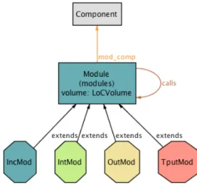
Listing 3.1 Alloy model for IIOT.
a b s t r a c t sig M o d u l e { v o l u m e : one L o C V o l u m e , m o d _ c o m p : one C o m p o n e n t , c a l l s : set M o d u l e
}
sig IntMod , IncMod , OutMod , T p u t M o d e x t e n d s M o d u l e {} sig C o m p o n e n t {}
sig L o C V o l u m e {} sig I I O T M o d e l {
m o d u l e s : M o d u l e }
This is a fairly simple model. We have two fundamental elements: components and modules. A component consists of several modules and these two entities are tied together by the mod_comp relation. It is worth noting that this relation connects each module to one and only onecomponent and its converse connects a component to a set of modules. As for the modules themselves, we used a simple inheritance mechanism to define the various types of modules that IIOT contemplates. There is also a calls relation that, obviously, defines which modules call which.
The construction of this model was straightforward. It was simply a matter of defining all the necessary sigs which came directly from the model definition. Later it was necessary to develop a series of predicates to express the various rules which were once again extracted from the model documentation.
Figure 3.1: Alloy metamodel for the IIOT model.
Interestingly, when defining the call rules for each of the module types, it was necessary to explicitly state not only the calls that a module must have but also the calls it cannot have. In the end, we defined 4 base predicates that define each of the 4 call types. They are shown in Listing 3.2.
Predicates NoCallsOutside and NotCalledOutside define the types of call that a mod-ule cannot have, either outbound or inbound. In the case of NoCallsOutside this is done by forcing all the called modules (mod.calls) to be a part of the same component. These are given by the fellows function: (mod.mod_comp) gives the module’s component while com-posing that with mod_comp gives the modules of the component. As for NotCalledOutside it uses the same rationale although applied inversely, ie, the modules that call the module in question belong to the same component.
The other two predicates (CalledOutside and CallsOutside) use a similar logic only forcing this time the called/calling modules to not be in the same component.
All these predicates are generic and can be applied to any module, though they only check a single module. Additional predicates that enforce them across the entire model are needed. They are shown in Listing 3.3.
3.1.3
Discussion
To begin our discussion of IIOT we present a list of related terminology.
Listing 3.2 General call rules for the IIOT Alloy model p r e d N o C a l l s O u t s i d e [ mod : M o d u l e ]{ mod . c a l l s in f e l l o w s [ mod ] } p r e d N o t C a l l e d O u t s i d e [ mod : M o d u l e ]{ c a l l s . mod in f e l l o w s [ mod ] } p r e d C a l l s O u t s i d e [ mod : M o d u l e ] { s o m e mod . c a l l s
mod . c a l l s not in f e l l o w s [ mod ] }
p r e d C a l l e d O u t s i d e [ mod : M o d u l e ] { s o m e c a l l s . mod
c a l l s . mod not in f e l l o w s [ mod ] }
fun f e l l o w s [ mod : M o d u l e ] : set M o d u l e { m o d _ c o m p .( mod . m o d _ c o m p )
}
are made up of modules.
Module: the lowest level partition of a software system in the IIOT model. A module typically
represents a source code file.
Module call: a relation between two modules, extracted from a software system’s call graph. Outbound call: the module call relation from the point of view of the calling module.
Mod-ules “make” outbound calls.
Inbound call: the converse of the outbound call relation. Modules “receive” inbound calls. Internal module: a module that only calls or is called by modules from the same
compo-nent.
Incoming module: a module where at least some inbound calls relate with modules from
other components and whose outbound calls only relate with modules from the same component.
Listing 3.3 Module type call rules for the IIOT Alloy model p r e d I n t e r n a l _ C a l l s [ i i o t : I I O T M o d e l ]{ all i n t M : I n t M o d | N o C a l l s O u t s i d e [ i n t M ] and N o t C a l l e d O u t s i d e [ i n t M ] } p r e d I n c o m i n g _ C a l l s [ i i o t : I I O T M o d e l ]{ all i n c M : I n c M o d | N o C a l l s O u t s i d e [ i n c M ] and C a l l e d O u t s i d e [ i n c M ] } p r e d O u t g o i n g _ C a l l s [ i i o t : I I O T M o d e l ]{ all o u t M : O u t M o d | N o t C a l l e d O u t s i d e [ o u t M ] and C a l l s O u t s i d e [ o u t M ] } p r e d T h r o u g h p u t _ C a l l s [ i i o t : I I O T M o d e l ]{ all t p u t M : T p u t M o d | C a l l e d O u t s i d e [ t p u t M ] and C a l l s O u t s i d e [ t p u t M ] } p r e d A l l _ P r e d s [ i i o t : I I O T M o d e l ]{ L o n e _ C o m p o n e n t [ i i o t ] I n t e r n a l _ C a l l s [ i i o t ] I n c o m i n g _ C a l l s [ i i o t ] O u t g o i n g _ C a l l s [ i i o t ] T h r o u g h p u t _ C a l l s [ i i o t ] }
Outgoing module: a module whose inbound calls only relate with modules from the same
component and where at least some outbound calls relate with modules from other components.
Throughput module: a module where at least some inbound and some outbound calls
relate with modules from other components.
Orphan module: a module that belongs to no component.
Inspecting several instantiations of the model unveils some interesting aspects which are worth discussing.
For instance, when classifying each of the module types there was a need to define both the types of calls a module can and cannot make.
There are several instances of modules calling themselves. While there can be some debate on the need to model these kinds of situations, it seems perfectly acceptable for them to exist.
Modules with no calls (inbound or outbound) are forcibly of type Internal. This is directly related to the definitions for the other types which all require the presence of calls. Only internal modules can have no calls and still respect their definition.
Another interesting point is that of orphan modules, which are modules that belong to no component. IIOT does not permit the existence of orphan modules. Though the model initially allowed for them, it was a simple matter to create an additional predicate to remove them.
In the end, it can safely be said that IIOT is a well built model. It is simple to understand (particularly since it exists at an abstraction level that is so close to the source code) and has no apparent contradictions. This understanding of the model seems more than sufficient to build a tool that incorporates it.
3.2
SIP Model
The SIP model was developed by Roger Sessions. It is used as part of a consulting business and its main purpose is to help reduce architectural complexity [60]
3.2.1
Model Description
SIP models the architecture of a software system from a functionality point of view. SIP is as much a process and a methodology as it is an architectural model. However, our purposes are focused strictly on the model. Additionally, though SIP is meant to model more than the SA (all the way up to the whole enterprise architecture) we simply use it for SA modeling. Because of this, we focus on a special version of SIP, which specializes in SOA. This version of SIP can easily be used to model a system’s SA.
The main elements of the SIP model we used are:
Component The topmost partition of a system. Systems are broken down into several
(top-level) components.
Functional group Represents a piece of functionality of the system (e.g. Make Payment or
Login).
As mentioned above, the primary purpose of SIP is to reduce SA complexity. A system is decomposed and organized into components. Relations in the form of dependencies exist between components. These dependencies manifest themselves when a functional group from one component depends on a functional group from another component. In this case, the first component depends on (or is related to) the second. We generally call these relations connections.
After the system has been modelled as a series of functional groups, the process of re-ducing it by partitioning can begin. Partitioning typically involves breaking a functional group into lower level ones. These functional groups are then grouped according to synergy (in other words, the “most similar” functional groups are placed together). Afterwards, these groups of functional groups are packed into the various components of the system. Finally, we establish the necessary connections between the various functional groups and, by ex-tension, components.
The proposed advantage of using SIP to assist in designing a system is that it leads to a system with the smallest amount of functional groups, components and connections. This in turn leads to lower complexity. This is because SIP argues that complexity is a function of the amount of functional groups and connections in the system.
SIP also includes a metric for measuring architectural complexity. This metric measures complexity as a function of the number of functional groups in each component and the number of connections between components. The metric is computed on a per-component
basis and then summed up to obtain the overall complexity of the system. This metric has an underlying mathematical basis and will be presented in chapter 5.
3.2.2
Alloy Analysis
It should be clear by now that SIP has a much greater focus on process than on the actual architectural model. In order to deepen our understanding of how an SA can be modelled in SIP we once again perform an analysis with Alloy. This gives us a better idea on how a SA looks like in SIP.
Listing 3.4 and Figure 3.2 represent a preliminary version of our Alloy model for SIP:
Listing 3.4 Alloy model for SIP.
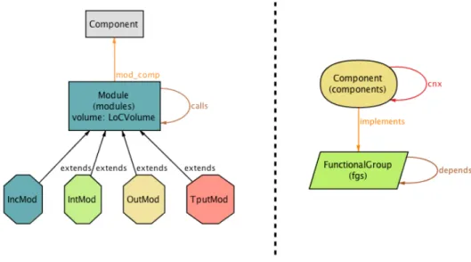
// - - Si g s a b s t r a c t sig S I P S y s t e m { fgs : set F u n c t i o n a l G r o u p , c o m p o n e n t s : set C o m p o n e n t } sig F u n c t i o n a l G r o u p { d e p e n d s : set F u n c t i o n a l G r o u p } sig C o m p o n e n t { cnx : set C o m p o n e n t , i m p l e m e n t s : set F u n c t i o n a l G r o u p }
As can be seen from the metamodel of Figure 3.2, the SIP model is a very simple one where a system is composed of components which are connected to each other via the cnx relation. In addition, there are various functional groups (modelled by FunctionalGroup)
that are packed into components. This is modelled with the implements relation. FunctionalGroups are also connected to each other, as modeled with the depends relation.
There is little in terms of predicates worth discussing in this model. This is because the model has no taxonomy or classification and therefore, has very few rules to follow. In fact, all the predicates written for this model were mostly related to ensuring the various relations behaved correctly (for example, there is a predicate to ensure that a component is not connected to itself).
Figure 3.2: Alloy metamodel for SIP model.
The only predicate worth mentioning is SIP_Depends_Connection_Rule, shown in List-ing 3.5.
Listing 3.5 Rule for component connections in the SIP Alloy model
// FG d e p e n d s = > C o m p o n e n t cnx
p r e d S I P _ D e p e n d s _ C o n n e c t i o n _ R u l e [ sip : S I P S y s t e m ]{
sip . c o m p o n e n t s <: cnx in sip . c o m p o n e n t s <: i m p l e m e n t s . d e p e n d s .~ i m p l e m e n t s
all d i s j fg1 , fg2 : sip . fgs | fg2 in fg1 . d e p e n d s and D i f f C o m p o n e n t [ fg1 , fg2 ] = > C o m p o n e n t C o n n e c t i o n [ fg1 , fg2 , sip ] } p r e d D i f f C o m p o n e n t [ fg1 , fg2 : F u n c t i o n a l G r o u p ]{ i m p l e m e n t s . fg1 not = i m p l e m e n t s . fg2 } p r e d C o m p o n e n t C o n n e c t i o n [ fg1 , fg2 : F u n c t i o n a l G r o u p , sip : S I P S y s t e m ]{ ( i m p l e m e n t s . fg2 ) in ( i m p l e m e n t s . fg1 ) . cnx }
This predicate simply ensures that all connections between components are a direct result of a dependence in their respective functional groups. This is achieved by forcing all regular connections between a system’s components ((sip.components <: cnx) to belong to implements.depends.˜ implements (relation between components whose func-tional groups have a dependence). Afterwards it is only a matter of stating that a dependence
from two functional groups of different components implies a connection between said com-ponents (all disj fg1, fg2 : sip.fgs | fg2 in fg1.depends
and DiffComponent[fg1,fg2] => ComponentConnection[fg1, fg2, sip]).
3.2.3
Discussion
Due to the simplicity of this model, there is not much worth investigating here. However there are still a few things worth exploring.
One aspect explored was the transitivity of the depends relation since it is not desirable for transitive dependencies to be explicitly and forcefully present. This is because all depen-dencies have a connection counterpart and these connections are going to be present in the source code. So an artificial increase in the connection count is not wanted.
The analysis of several instances of the model shows a variety of situations though noth-ing quite worth discussnoth-ing or explornoth-ing further. However, it does give us an increased con-fidence in our model and our understanding of SIP. Since the model is so simple it is fairly easy to understand. However, this type of analysis is always useful to deepen comprehen-sion, if only by a small amount.
3.3
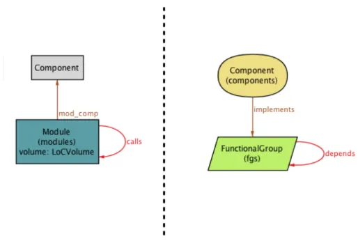
Unification
This section shows how to bridge both models into a single, unified model. As it turns out, this is actually quite simple. The purpose of this unification is to be able to take the complexity metric calculation feature from SIP and apply it to IIOT. In order to do this, we must build an intermediate model of some sort (called SIPI for now). This model has two requirements:
• It must be possible to build the model either from a IIOT model or the base information used to build such an IIOT model (a call graph).
• This model must contain all the information of a SIP model for the same system, so as to enable complexity calculation.
Putting both metamodels side by side, as shown in Figure 3.3, we already see a great number of similarities between them. These can be increased even further by discarding a few elements from each model. On the IIOT side, module classifications can be ignored as