Mineração de padrões de correlação estrutural em grandes grafos

(1)

MINERA ¸

C ˜

AO DE PADR ˜

OES DE CORRELA ¸

C ˜

AO

(2)

(3)

ARLEI LOPES DA SILVA

MINERA ¸

C ˜

AO DE PADR ˜

OES DE CORRELA ¸

C ˜

AO

ESTRUTURAL EM GRANDES GRAFOS

Disserta¸cão apresentada ao Programa de Pós-Gradua¸cão em Computer Science do Instituto de Ciências Exatas da Universi-dade Federal de Minas Gerais como req-uisito parcial para a obten¸cão do grau de Mestre em Computer Science.

Orientador: Wagner Meira Jr.

(4)

(5)

ARLEI LOPES DA SILVA

STRUCTURAL CORRELATION PATTERN

MINING FOR LARGE GRAPHS

Dissertation presented to the Graduate Program in Computer Science of the Uni-versidade Federal de Minas Gerais in par-tial fulfillment of the requirements for the degree of Master in Computer Science.

Advisor: Wagner Meira Jr.

(6)

Silva, Arlei Lopes da

S586m Minera¸cão de Padrões de Correla¸cão Estrutural em Grandes Grafos / Arlei Lopes da Silva. — Belo Horizonte, 2011

xxvi, 128 f. : il. ; 29cm

Disserta¸c˜ao (mestrado) — Universidade Federal de Minas Gerais

Orientador: Wagner Meira Jr.

1. Computa¸c˜ao – Teses. 2. Minera¸c˜ao de dados – Teses. 3. Teoria dos grafos. Teses. I. Orientador. II. T´ıtulo.

(7)

(8)

(9)

Acknowledgements

First of all, I would like to thank my advisor Wagner Meira Jr. for his collabo-ration over the past 5 years. I was an undergrad student with average grades when I knocked Meira’s door to ask him for a position as an undergrad researcher. Since then, he has provided me with many opportunities to learn the skills I needed to finish this thesis and to progress in my career as a computer scientist.

I would also like to thank Mohammed J. Zaki for his guidance during the 6 months I have spent as a visiting scholar at RPI and for the collaboration that followed. Most of the technical contributions of this thesis were a consequence of my attempts to address some of his comments. Thanks also to Lo¨ıc Cerf and Alberto Laender who were part of my thesis committee and contributed to the improvement of this work.

I am honored to have worked with Adriano Pereira, Fabio Figueiredo, Fernando Mourão, Herico Valiati, Jussara Almeida, Leonardo Rocha, Livia Simões, Lo¨ıc Cerf, Marco Ribeiro, Marcos Gon¸calves, Mariângela Cherchiglia, Mehdi Kaytoue, Nathan Mariano, Odilon Queiroz, Pedro Calais, Walter Santos and Sara Guimarães. I would like to give my special thanks to Adriano for his generous support since my first years as an undergrad researcher.

Being a mastering student is much better when you have some good friends, such as Carlos Teixeira and Charles Gon¸calves, around. Thanks also to all my colleagues from the e-Speed Lab, where I have spent a significant part of the past 5 years. In particular, I would like to thank Bruno Coutinho for his always kind helping. Thanks also to the staff from the Computer Science Department, specially Cida and Sˆonia, for the patience and sympathy, despite of my constant lack of organization.

While I was a high school student at Cidade dos Meninos, many teachers mo-tivated me to study hard to get into college, such as Julio, Adalberto, Katia, and Glauceones. I am also grateful to Jairo Azevedo, founder of Cidade dos Meninos, and the numerous contributors that support the APHDP.

During most of my undergraduate studies, I was assisted by the community from Universidade Federal de Minas Gerais through Funda¸c˜ao Mendes Pimentel.

I have always received support and encouragement from my family and friends, specially my mother Ivone, my brother Andre, my friend David and my brother Alex, without whom I would never get anywhere close to this.

(10)

(11)

“Dubium sapientiae initium.”

(Latin proverb)

(12)

(13)

Resumo

Grafos têm se estabelecido como um poderoso arcabou¸co teórico para a modelagem de intera¸cões em cenários variados. Enquanto a disponibilidade de dados em larga escala motivou o desenvolvimento de tal arcabou¸co, o enriquecimento desses dados guia a pesquisa em grafos na dire¸cão de novos métodos capazes de explorar essa riqueza de forma útil. Uma representa¸cão estendida interessante de grafos é a de grafos com atributos nos vértices. Atributos de vértices desempenham um papel importante em diversos grafos reais. Além disso, sabe-se que, em muitos desses grafos, vértices se organizam naturalmente como subgrafos densos. Tais subgrafos possuem signficado relevante em diversos grafos reais, sendo denominados comunidades em redes sociais e identificando complexos proteicos em redes de prote´ınas, dentre outras aplica¸cões.

Neste trabalho, estudamos a correla¸cão entre conjuntos de atributos e a forma¸cão de subgrafos densos, o que denominamos minera¸cão de padrões de correla¸cão estrutural. A correla¸cão estrutural mede como um conjunto de atributos induz subgrafos densos em grafos com atributos. Um padrão de correla¸cão estrutural é um subgrafo denso induzido por um conjunto de atributos em particular. Modelamos padrões de correla¸cão estrutural em termos de padrões de minera¸cão de dados existentes. Com base em tal modelagem, propomos técnicas de normaliza¸cão que avaliam o quanto a correla¸cão estrutural de um conjunto de atributos desvia do esperado. Além disso, propomos algoritmos eficientes e escaláveis para a minera¸cão de padrões de correla¸cão estrutural. Nós mostramos que a minera¸cão de padrões de correla¸cão estrutural é capaz de prover conhecimento relevante sobre a rela¸cão entre conjuntos de atributos e subgrafos densos em grafos reais. Em particular, aplicamos os algoritmos propostos na correla¸cão entre palavras-chave associadas a pesquisadores e a forma¸cão de grupos de pesquisa em redes de colabora¸cão, no estudo de comunidades induzidas pelo gosto musical em uma rede social, na análise de como grupos conectados de artigos emergem em torno de tópicos de pesquisa em uma rede de cita¸cão, e na avalia¸cão da rela¸cão entre expressão e funcionalidade em uma rede de intera¸cão proteica. Também avaliamos o desempenho de tais algoritmos, verificando que eles possibilitam a análise de grandes bases de dados.

(14)

(15)

Abstract

Graphs have been established as a powerful theoretical framework for modeling several types of interactions in a variety of scenarios. While the availability of large scale data led to the development of a framework for large scale graph analysis, the enrichment of such data drives the graph research to new methods able to explore such richness in a useful manner. An interesting extended graph representation is called attributed graph. Vertex attributes play an important role in several real life graphs. Moreover, it is broadly known that in several of these graphs vertices are organized into dense subgraphs. Such subgraphs have a relevant meaning in several real life graphs, being called communities in social networks and identifying protein complexes in protein-protein interaction networks.

In this work, we study the correlation between attribute sets and the formation of dense subgraphs in large attributed graphs, which we call structural correlation pattern mining. The structural correlation measures how a set of attributes induces dense subgraphs in attributed graphs. A structural correlation pattern is a dense subgraph induced by a particular attribute set. We model the structural correlation pattern mining in terms of existing data mining patterns. Based on such definitions, we propose normalization approaches in order to assess how the structural correlation of a given attribute set deviates from the expected. Moreover, we propose efficient and scalable algorithms for structural correlation pattern mining.

We show that the structural correlation pattern mining is able to provide rele-vant knowledge about the relation between attribute sets and dense subgraphs in real attributed graphs. In particular, we apply the proposed algorithms to the correlation between keywords associated with researchers and the formation of research groups in collaboration networks, in the study of communities induced by musical taste in a social network, in the analysis of how well connected groups of papers emerge around research topics in a citation network, and in the evaluation of the relation between expression and functionality in a PPI network. We also evaluate the performance of such algorithms, verifying that they enable the analysis of large datasets.

(16)

(17)

List of Figures

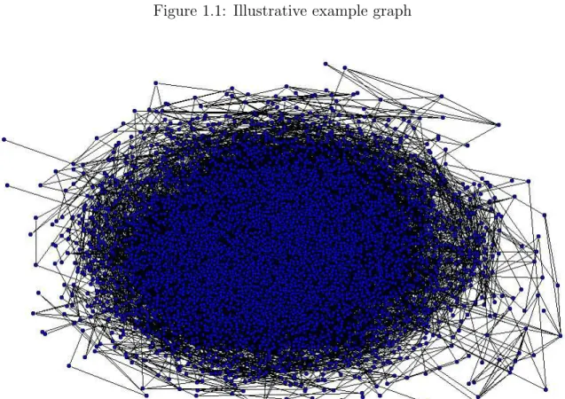
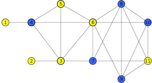
1.1 Illustrative example graph . . . 2

1.2 Co-authorship graph extracted from the DBLP digital library . . . 2

1.3 Dense subgraph from the graph shown in Figure 1.1 . . . 5

1.4 Dense subgraph from the graph shown in Figure 1.1 . . . 6

1.5 Dense subgraph from the real graph shown in Figure 1.2 . . . 7

2.1 Set Enumeration Tree . . . 16

2.2 Subgraph of the quasi-clique shown in Figure 1.3 which is not a 0.6-quasi-clique . . . 16

2.3 Complete lattice for the set of attributes {A, B, C, D, E} . . . 24

3.1 Graph from Figure 1.1, vertices 3 to 11 have the attribute A and are in dense subgraphs, vertices 1 and 2 have the attribute Abut are out of dense subgraphs . . . 29

3.2 Graph from Figure 1.1, vertices 1, 3, and 6 have the attribute C and the other vertices do not have C . . . 30

3.3 Graph from Figure 1.1, vertices 6 to 11 have the attribute set {A, B} and are in dense subgraphs, the other vertices do not have {A, B} . . . 30

3.4 Graph induced by the attribute set {search, rank} from the collaboration graph shown in Figure 1.2. . . 31

3.5 Clique with the same number of vertices that the graph shown in Figure 1.1 33 4.1 Order of visit of candidate patterns in a BFS search . . . 48

4.2 Order of visit of candidate patterns in a DFS search . . . 48

5.1 Cumulative degree, attribute frequency, and attributes per vertex distribu-tion (in log-log scale) for the DBLP dataset . . . 75

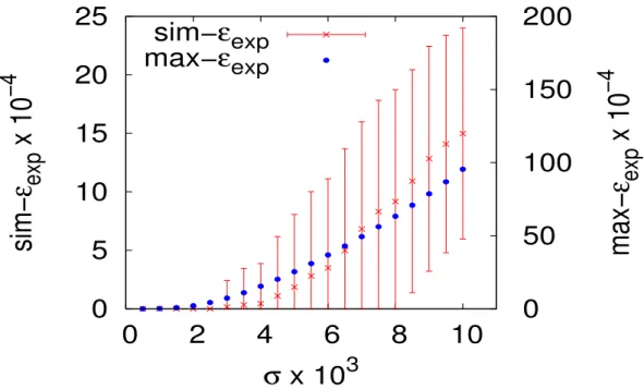
5.2 Expected structural correlation computed using the simulation model (sim-ǫexp) and the analytical model max-ǫexp . . . 77

(18)

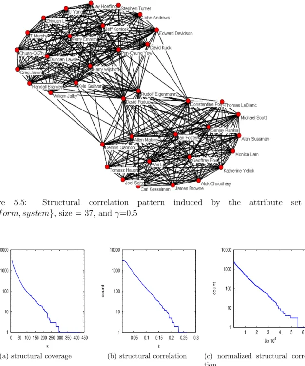
size = 13, and γ=0.58 . . . 79 5.5 Structural correlation pattern induced by the attribute set

{perf orm, system}, size = 37, and γ=0.5 . . . 80 5.6 Inverse cumulative structural coverage (κ), structural correlation (ǫ), and

normalized structural correlation (δ2) . . . 80 5.7 Inverse cumulative degree, attribute frequency, and attributes per vertex

distribution (in log-log scale) for the LastFm dataset . . . 82 5.8 Expected structural correlation computed using the simulation model

(sim-ǫexp) and the analytical model max-ǫexp . . . 84

5.9 Graph induced by the attribute set{Sufjan Stevens, Wilco}in the LastFm dataset . . . 85 5.10 Structural correlation pattern induced by the attribute set{Sufjan Stevens,

Wilco}, size = 11, and γ=0.7 . . . 86 5.11 Structural correlation pattern induced by the attribute set{Van Morrison},

size = 34, and γ=0.52 . . . 86 5.12 Inverse cumulative structural coverage (κ), structural correlation (ǫ), and

distributions (in log-log scale) for the CiteSeer dataset . . . 89 5.14 Expected structural correlation computed using the simulation model

5.15 Graph induced by the attribute set {node, wireless} in the CiteSeer dataset 91 5.16 Structural correlation pattern induced by the attribute set{node, wireless},

size = 9, and γ=0.5 (EEBAWN - Energy-efficient Broadcasting in All-wireless networks, SAEECATMAWN - Span: An Energy-efficient Coor-dination Algorithm for Topology Maintenance in Ad-hoc Wireless works, ECRWAN - Energy-conserving Routing in Wireless Ad-hoc Net-works, MEMWN - Minimum-Energy Mobile Wireless NetNet-works, CMCP-WSN - Connectivity Maintenance and Coverage Preservation in Wireless Sensor Networks, GIECAR - Geography-informed Energy Conservation for Ad-hoc Routing, MEBAWN - Minimum-energy Broadcast in All-wireless Networks, DTCWSNDCPEOMWAN - Distributed Topology Control in Wireless Sensor Networks with Distributed Control for Power-efficient Op-eration in Multihop Wireless Ad-hoc Networks) . . . 92

(19)

5.17 Structural correlation pattern induced by the attribute set

{perf orm, system}, size = 21, and γ=0.5 (AC - Attribute Caches, SLCM - Systems for Late Code Modification, OTDRN - Observing TCP Dynamics in Real Networks, TCIG - Transparent Controls for Interactive Graphics, LILP Limits of Instruction Level Parallelism, DLMR -DECWRL/Livermore Magic Release, LTOAC6BA - Link-time Optimiza-tion of Address CalculaOptimiza-tion on a 64-bit Architecture, LTCM - Link-time Code Modification, MSDCDSP - Memory-system Design Considerations for Dinamically Scheduled Processors, BMFCEG - Boolean Matching for Full-custom ECL Gates, CWPP - Cache Write Policies and Performance, SMCM - Shared Memory Consistency Models, CEFCGASDSM - Com-parative Evaluation of Fine and Coarse-grain Approaches for Software Distributed Shared Memory, RLG - Recursive Layout Generation, EDPP - Efficient Dynamic Procedure Placement, DSDI - Drip: A Schematic Drawing Interpreter, FPPDMA - Fluoroelastomer Pressure Pad Design for Microelectronic Applications, TTOCC - Trade-offs in Two-level on-chip Caching, IOCCIOCD - I/O Component Characterization for I/O Cache Designs, VMFS - Virtual Memory vs File System, EWWWWC - Experience with a Wireless World Wide Web Client) . . . 93 5.18 Inverse cumulative structural coverage (κ), structural correlation (ǫ), and

distributions (in log-log scale) for the Human dataset . . . 96 5.20 Graph induced by the attribute set{+SHCN086,+SHCN087,+SHCN088}

in the Human dataset . . . 97 5.21 Structural correlation pattern induced by the attribute set

{+SHCN086,+SHCN087,+SHCN088}, size = 7, and γ=0.5 . . . 98 5.22 Expected structural correlation computed using the simulation model

5.23 Cumulative structural coverage (κ), structural correlation (ǫ), and normal-ized structural correlation (δ2) . . . 100 5.24 Parameter sensitivity w.r.t the minimum structural correlation (ǫmin) . . . 102

5.25 Parameter sensitivity w.r.t the minimum normalized structural correlation (δmin) . . . 103

5.26 Runtime of SCPM-BFS, Naive and SCPM-DFSw.r.t. γmin . . . 105

5.27 Runtime of SCPM-BFS, Naive and SCPM-DFSw.r.t. min size . . . 105 5.28 Runtime of SCPM-BFS, Naive and SCPM-DFSw.r.t. σmin . . . 106

(20)

5.31 Runtime of SCPM-DFS, SCPM-BFS-SAMP and SCPM-DFS-SAMP w.r.t. θmax . . . 109

5.32 Mean squared error of SCPM-SAMP-DFS w.r.t. θmax . . . 109

5.33 Runtime of theSCPM-DFSand the Naive algorithm w.r.t. k . . . 110 5.34 Runtime and speedup of PAR-SCPM-DFS w.r.t. the number of cores . 111 5.35 Runtime and speedup of PAR-SCPM-BFSw.r.t. the number of cores . 112 5.36 Runtime and speedup of thePAR-SAMP-SCPM-BFSw.r.t. the number

of cores . . . 112 5.37 Runtime and speedup of thePAR-SAMP-SCPM-DFSw.r.t. the number

of cores . . . 113

(21)

List of Tables

1.1 Attributes of the vertices from the graph shown in Figure 1.1 . . . 5

2.1 Frequent attribute sets from the vertex attributes shown in Table 1.1 (the minimum support set is 3) . . . 24

3.1 Table of Symbols . . . 29

3.2 Number of possible settings, expected structural correlation (ǫexp),

simulation-based structural correlation (sim-ǫexp), and analytical

normal-ized structural correlation (max-ǫexp) forN randomly selected vertices from

the graph 1.1 . . . 34

3.3 Attribute sets, with their respective values of σ, κ, and ǫ, from the graph shown in Figure 1.1, for which the vertex attributes are presented in Table 1.1 if σmin = 3, γmin = 0.6,min size= 4, and ǫmin = 0.5 . . . 40

3.4 Structural correlation patterns, with their respective sizes (size) and densi-ties γ, from the graph shown in Figure 1.1, for which the vertex attributes are presented in Table 1.1 if σmin = 3, γmin = 0.6, min size = 4, and

ǫmin = 0.5 . . . 41

3.5 Attribute sets, with their respective values ofσ,κ,ǫ, max-ǫexp, andδ2, from the graph shown in Figure 1.1, for which the vertex attributes are presented in Table 1.1 if σmin = 3, γmin = 0.6, min size= 4, and δmin = 1.0 . . . 42

3.6 Structural correlation patterns, with their respective sizes (size) and densi-ties γ, from the graph shown in Figure 1.1, for which the vertex attributes are presented in Table 1.1 if σmin = 3, γmin = 0.6, min size = 4, and

δmin = 1 . . . 42

5.1 Top-ǫ attribute sets from DBLP . . . 76

5.2 Top-δ2 attribute sets from DBLP . . . 77

(22)

ferent attribute set sizes (|S|) in the DBLP dataset . . . 81 5.4 Top-ǫ attribute sets from the LastFm dataset . . . 83 5.5 Top-δ2 attribute sets from the LastFm dataset . . . 84 5.6 Scatter plots of the correlations between support (σ), structural coverage

(κ), structural correlation (ǫ), and normalized structural correlation for dif-ferent attribute set sizes (|S|) in the LastFm dataset . . . 88 5.7 Top-ǫ attribute sets from CiteSeer . . . 90 5.8 Top-δ2 attribute sets from the CiteSeer dataset . . . 91 5.9 Scatter plots of the correlations among support (σ), structural coverage (κ),

structural correlation (ǫ), and normalized structural correlation for different attribute set sizes (|S|) in the CiteSeer dataset . . . 95 5.10 Top-ǫ attribute sets from the Human dataset . . . 97 5.11 Top-δ2 attribute sets from the Human dataset . . . 100 5.12 Scatter plots of the correlations among support (σ), structural coverage (κ),

structural correlation (ǫ), and normalized structural correlation for different attribute set sizes (|S|) in the Human dataset . . . 101

(23)

List of Algorithms

1 Set Enumeration Tree Algorithm . . . 18 2 extend . . . 19 3 Simulation Null Model for the Structural Correlation Algorithm . . . . 35 4 Naive Algorithm For Structural Correlation Pattern Mining . . . 47 5 structural-correlation . . . 49 6 coverage-BFS . . . 49 7 coverage-DFS . . . 50 8 structural-correlation-with-sampling . . . 54 9 check-vertex-in-quasi-clique . . . 55 10 find-quasi-clique-BFS . . . 55 11 find-quasi-clique-DFS . . . 56 12 top-k-structural-correlation-patterns . . . 56 13 try-to-update-top-patterns . . . 58 14 SCPM Algorithm . . . 59 15 enumerate-patterns . . . 60 16 par-structural-correlation . . . 62 17 par-coverage-BFS . . . 63 18 par-coverage-DFS . . . 64 19 par-coverage . . . 65 20 par-check-vertex-in-quasi-clique . . . 66 21 par-find-quasi-clique-BFS . . . 67 22 par-find-quasi-clique-DFS . . . 68 23 par-find-quasi-clique . . . 69 24 par-top-k-structural-correlation-patterns . . . 69 25 par-top-k-scps-thread . . . 70 26 par-top-k-scps-iteration . . . 71 27 par-try-to-update-top-patterns . . . 72

(24)

(25)

5.1 Case Studies . . . 74 5.1.1 DBLP . . . 75 5.1.2 LastFm . . . 82 5.1.3 CiteSeer . . . 88 5.1.4 Human . . . 96 5.2 Parameter Sensitivity and Setting . . . 102 5.3 Performance Evaluation . . . 103 5.3.1 Computing the Structural Correlation . . . 104 5.3.2 Sampling . . . 107 5.3.3 Discovering the Top-K Structural Correlation Patterns . . . 109 5.3.4 Parallel Algorithms . . . 110 5.3.5 Discussion . . . 113

6 Conclusions 115

6.1 Summary of Contributions . . . 115 6.2 Limitations . . . 116 6.3 Future Work . . . 117

Bibliography 121

(27)

Chapter 1 Introduction

Graphs, or networks, have been established as a powerful theoretical framework for modeling several types of interaction in a variety of scenarios. Due to its broad ap-plicability, graphs have attracted a great interest from a wide research community, including mathematicians, physicists, sociologists, biologists, and computer scientists. The availability of large real graphs in the last years motivated a broad spectrum of re-search on the properties of such graphs. Moreover, the combination of new algorithms and powerful hardware have enabled the discovery of complex and interesting patterns from large graphs.

A graph is usually defined as a set of vertices (or nodes) connected by a set of

edges. Figure 1.1 shows an illustrative example of a graph with 11 vertices (1-11) and 21 edges. Figure 1.2 is a real graph extracted from a digital library. Each vertex represents an author and two vertices are connected if their respective authors have already collaborated on a paper. From social networks to food webs, from distribution networks to the WWW, many relevant systems can be modeled through graphs.

The study of graphs has evolved significantly since the solution of the Konigs-berg problem by Euler in 1735, which is considered the first scientific work on graphs in the literature. While the first studies were focused on graph theory, subsequent studies applied graphs to the analysis of small social networks. The seminal Milgram’s paper [Travers and Milgram, 1969], for example, showed that randomly selected indi-viduals from Boston and Nebraska were connected to randomly selected people from Massachusetts through a connected chain of acquaintances of average size 5.2, what is considered the first evidence of the so called small world phenomenon. However, along the past few years, the study of graphs has witnessed a new shift in the direction of the analysis of large scale statistical properties of real graphs [Newman, 2003]. An ex-tensive study of several real graphs from different domains have shown that interesting

(28)

Figure 1.1: Illustrative example graph

Figure 1.2: Co-authorship graph extracted from the DBLP digital library

properties (e.g., power-law degree distributions, high clustering coefficient, community structure, and small diameter) are common to many of these graphs.

(29)

3

graphs. A significant part of the research community on graphs has agreed that the graph research is evolving towards more complex models and analysis [Newman, 2003; Leskovec, 2008; Chakrabarti and Faloutsos, 2006].

Along its two centuries of history, the study of graphs has shifted from theory to application, and then to large scale. However, a simple undirected graph (see Figure 1.1) has remained as the standard model on graph research. Such a simple model is popular for two basic reasons: (1) it is powerful enough for the analysis of topological static properties of graphs (e.g., degree distribution, clustering coefficient) and (2) it is simple for both understanding and computational processing. Nevertheless, in recent years, the availability of rich data from complex scenarios has motivated analyses that are far beyond static topological properties.

Extending the standard simple graph framework is, in general terms, the topic of this work. While the availability of large scale data led to the development of a framework for large scale graph analysis, the availability of rich data drives the graph research to new methods able to explore such data in a useful manner. Graphs with directed, weighted, multi-typed, and attributed edges, for example, may provide novel interesting knowledge in several application scenarios. Similarly, vertices may have multiple types and attributes. Moreover, some scenarios require the study of multiple graphs or even several snapshots of the same graph, instead of a single static graph. Extracting useful knowledge from such complex large datasets brings new challenges not only in terms of modeling but also efficiency and scalability. In order to address such challenges, a new branch of data mining known as graph mining has attracted great attention of the data mining community in recent years.

(30)

1.1 Structural Correlation Pattern Mining

This work studies the problem of correlating vertex attributes and the existence of dense subgraphs in an attributed graph (i.e., a graph where vertices have attributes). We call this problem structural correlation pattern mining, since it correlates vertex attributes and a structural (or topological) information from graphs.

Vertex attributes play an important role in several real life graphs. In social networks, vertex attributes are useful to represent personal characteristics (e.g., age, gender, interests). In protein-protein interaction networks, vertex attributes can rep-resent expression or annotation data. Moreover, vertex attributes can be associated to content (e.g., keywords, tags) in the web graph. Table 1.1 shows attributes of vertices from the illustrative example graph shown in Figure 1.1. Each attribute is represented through a letter in the interval A-E. Attributes for vertices shown in Figure 1.2 can be keywords associated to each researcher and can represent their topics of interest.

It is broadly known that in several real graphs vertices are naturally organized into dense subgraphs [Fortunato, 2010]. Dense subgraphs are sets of vertices with high cohesion (i.e., strong connections among themselves). Such subgraphs carry an important meaning in several real life scenarios. In social networks, people interact more intensely inside communities, what is of great interest in social sciences [Newman, 2003; Scott, 2000; Carrington, 2005]. Web pages usually contain links to other related pages, resulting in cyber-communities of pages and sites sharing a common interest [Albert et al., 1999; Dourisboure et al., 2009]. Densely connected proteins in protein-protein interaction networks define molecular complexes that are useful for functional annotation [Spirin and Mirny, 2003]. Groups of publications citing each other can define the related work around a established research topic [Shi et al., 2010]. Detecting and analyzing dense subgraphs has been a long term research problem.

Figures 1.3 and 1.4 are two examples of dense subgraphs identified from the graph shown in Figure 1.1. The subgraph from Figure 1.3 is a clique (i.e., a set of vertices where there is an edge between each pair of vertices). A clique is the densest possible subgraph for a given set of vertices. The subgraph shown in Figure 1.4 is not a clique, but it has a high density (or cohesion), since only three pairs of vertices are not adjacent. Figure 1.5 is a dense subgraph extracted from the graph shown in Figure 1.2, it represents a group of researchers with several internal collaborations.

(31)

1.1. Structural Correlation Pattern Mining 5

graph analysis has being argued to enable the discovery of novel interesting knowledge from graphs, specially in the data mining and the bioinformatics literature [Silva et al., 2010, 2012; Ge et al., 2008; Moser et al., 2007, 2009; Pei et al., 2005; Zeng et al., 2006; Zhou et al., 2009].

vertex attributes

1 A, C

2 A

3 A, C, D

4 A,D

5 A, E

6 A, B, C

7 A, B, E

8 A, B

9 A, B

10 A, B, D

11 A, B

Table 1.1: Attributes of the vertices from the graph shown in Figure 1.1

Figure 1.3: Dense subgraph from the graph shown in Figure 1.1

(32)

Figure 1.4: Dense subgraph from the graph shown in Figure 1.1

inside dense subgraphs. The graph induced by an attribute set is composed by the ver-tices that have such attribute set and the edges between these verver-tices. The structural correlation of a given attribute set is the probability of a vertex to be member of a dense subgraph inside the graph induced by such an attribute set.

Considering the graph shown in Figure 1.1, the vertex attributes shown in Table 1.1 and the dense subgraphs shown in Figures 1.3 and 1.4, the structural correlation of the attribute C is 0, since there is no dense subgraph inside the graph induced by the attribute C (i.e., vertices 1, 3, and 6). The structural correlation of the attribute set {A,B} is 1, due to the fact that every vertex is a member of a dense subgraph in the graph induced by {A,B}. From the collaboration graph shown in Figure 1.2, taking the keywords from the tittle of the papers of each researcher as their attributes, and considering a dense subgraph a vertex set in which each vertex is connected to, at least, half of its other members, the structural correlation of the keyword “search” is 0.25 (i.e., 25% of the authors with the keyword “search” are members of dense subgraphs composed of other authors who also have this keyword). Therefore, the structural correlation can measure how keywords induce research groups in a collaboration graph. While the structural correlation is a property of an attribute set, a struc-tural correlation pattern is a pair (attribute set, dense subgraph). The pair ({A,B},

(33)

There-1.1. Structural Correlation Pattern Mining 7

Figure 1.5: Dense subgraph from the real graph shown in Figure 1.2

fore, such a pattern may represent a research group related to the topic web search. Both the structural correlation function and the structural correlation pattern definitions are based on two related hypotheses:

1. Attributes produce dense subgraphs;

2. Dense subgraphs affect the attributes of their internal vertices.

(34)

The correlation between attribute sets and the existence of dense subgraphs is not expected to be completely deterministic or completely random. Therefore, it is important to provide interestingness measures for the structural correlation based on how a given value of correlation deviates from the expected. In this work, we propose two null models for the structural correlation function. Such models provide the ex-pected structural correlation for a given attribute set assuming that attributes are set to vertices randomly.

We define the structural correlation pattern mining in terms of two existing data mining patterns: frequent itemsets and quasi-cliques. Frequent itemsets are applied in order to deal with the large number of possible attribute sets in real attributed graphs and quasi-cliques are used as a definition for dense subgraphs. In order to provide efficient and scalable algorithms for the proposed problems we combine existing strategies for frequent itemset and quasi-clique mining with new pruning, sampling and parallelization strategies specific for the structural correlation.

The structural correlation pattern mining constitutes a new graph analysis tech-nique for attributed graphs. It provides knowledge at the level of attribute sets, mea-suring how they are correlated to the existence of dense subgraphs in the graph, and also at the level of the subgraphs induced by the attribute sets (i.e., the structural cor-relation patterns). Such a knowledge may be applied to many real graphs from several domains, including social, information, and biological networks.

1.2 Contributions of This Work

The main contributions of this work are summarized as follows:

• Problem statement: We introduce the general problem of correlating vertex attributes and the existence of dense subgraphs in attributed graphs. As far as we know, there is no previous work on this problem in the literature.

• Modeling: Based on the statement of the problem, we define a structural corre-lation function and a structural correcorre-lation pattern combining two existing data mining patterns (frequent itemsets and quasi-cliques).

(35)

1.3. Outline 9

• Application and evaluation: We apply the structural correlation pattern min-ing to several real datasets from different domains. Usmin-ing such datasets, we eval-uate the performance of the proposed algorithms. We also conduct case studies in order to show the applicability of the structural correlation pattern mining in real-life scenarios.

1.3 Outline

The remaining of this work is organized as follows:

• Chapter 2 [Background]: Summarizes existing knowledge related to the struc-tural correlation pattern mining: dense subgraphs, quasi-clique mining, and fre-quent itemset mining. It also gives an overview on related work in the literature.

• Chapter 3 [Structural Correlation Pattern Mining: Definitions]: Gives formal definitions for the structural correlation function and structural correlation pattern mining.

• Chapter 4 [Structural Correlation Pattern Mining: Algorithms]: De-scribes algorithms for structural correlation pattern mining.

• Chapter 5 [Experimental Evaluation]: Presents case studies of the applica-tion of the structural correlaapplica-tion pattern mining in real-life scenarios and also an experimental evaluation of the proposed algorithms in terms of performance

(36)

(37)

Chapter 2 Background and Related Work

In this chapter we present an overview on important topics related to the structural correlation pattern mining: dense subgraphs and the quasi-clique and frequent itemset mining problems. Moreover, we discuss existing work related to the structural corre-lation pattern mining from the literature. The structural correcorre-lation pattern mining correlates attribute sets and the existence of dense subgraphs in an attributed graph. While the concept of attribute set is quite simple (a set of attributes), there is no single formal definition for a dense subgraph in the literature. There are several definitions for dense subgraphs and we survey some of them in Section 2.1. Among the existing definitions for dense subgraphs, we selected the quasi-clique definition. Section 2.2 de-scribes the quasi-clique mining problem and present many existing pruning techniques for the efficient identification of quasi-cliques in graphs. Understanding such techniques is important, since we employ them in the algorithms presented in Chapter 4. In Sec-tion 2.3, we overview the frequent itemset mining problem. We apply frequent itemset mining in order to select frequent attribute sets in the structural correlation pattern mining. Section 2.4 discusses related work on the structural correlation pattern mining.

2.1 Dense Subgraphs

The dense subgraph discovery is a multidisciplinary problem with great importance in physics, sociology, biology and computer science. Graphs can represent several com-plex real systems and understanding how vertices are organized into dense subgraphs has been a popular research topic. In social networks, where vertices represent people and edges represent social relationships (e.g., friendship, marriage, co-working), dense subgraphs are of special interest, since they constitute communities [Scott, 2000; Car-rington, 2005]. The World Wide Web can also be modeled as a graph, where pages

(38)

interact through hyperlinks. Dense subgraphs in the web graph are groups of pages sharing topic similarities (a.k.a. cyber-communities) [Dourisboure et al., 2009]. More-over, dense subgraphs can also represent an effort in order to enhance the PageRank [Brin and Page, 1998] of web pages artificially [Gy¨ongyi and Garcia-Molina, 2005]. Sim-ilar to web pages, publications can be connected through citations and dense subgraphs are useful for the discovery of topic-related publications. In biology and bioinformatics, the study of protein-protein interaction (PPI) networks is of special interest [Spirin and Mirny, 2003]. Proteins interact in biological processes in the cells and dense subgraphs correspond to functional groups (i.e., proteins with similar functions) in this scenario. The concepts of dense subgraph and graph community (a.k.a graph cluster) are close related. A community is usually defined as a set of vertices significantly more connected among themselves than with vertices outside it [Girvan and Newman, 2002; Newman, 2003; Puig-Centelles et al., 2008; Newman, 2004; Fortunato, 2010]. Therefore, a community is a dense subgraph, but a dense subgraph is not necessarily a community, because dense subgraphs can also have a strong cohesion with the rest of the graph. Such distinction between dense subgraphs and communities is not clear in the literature and the use of both concepts interchangeably is not uncommon. In general, dense subgraphs are exact definitions while communities are based on heuristics. Moreover, most of the algorithms for community identification restrict each vertex to be member of a single community (i.e., such algorithms identify graph partitions).

In this work, we apply a specific dense subgraph identification method (see Section 2.2) in order to compute the correlation between attribute sets and the formation of dense subgraphs. However, it is known that the definition of a dense subgraph may depend on the specific application scenario [Fortunato, 2010]. Although we try to generalize the concept of dense subgraph as much as possible, it is important to notice that some definitions of dense subgraphs can not be applied to our study. We define two requirements for a dense subgraph identification method to be applied to the correlation between attribute sets and the formation of dense subgraphs:

1. Detecting overlapping dense subgraphs: It is known that, in real graphs, vertices are shared between dense subgraphs. In social networks, for example, individuals can be members of different social circles. Restricting vertices to be members of a single dense subgraph leads to the neglection of potentially relevant information [Fortunato, 2010].

(39)

2.1. Dense Subgraphs 13

et al., 2007; Chakrabarti, 2004], which are vertices that do not belong to any dense subgraph, it is a general assumption that such cases are exceptions. However, our objective is to measure how attribute sets induce dense subgraphs and it is expected that in real graphs some attribute sets induce graphs for which the probability of a vertex to be in a dense subgraph is low.

In the remaining of this section we give several examples of dense subgraph defini-tions that could be applied in the correlation between attribute sets and dense subgraph formation. The simplest and most popular of them is a clique [Scott, 2000]. A set of vertices V is a clique if there is an edge between each pair of vertices inV. Cliques of interest are usually maximal subgraphs (i.e., they are not subsets of any other clique). Vertices can be naturally members of multiple cliques. However, the clique definition is too strict for real networks, which are known to be sparse [Newman, 2003]. As a consequence, large cliques are expected to be infrequent in real graphs.

There are several relaxations of the clique definition in the literature. A quasi-clique (see Section 2.2) is a set of vertices V such that each vertex is adjacent to a fraction γ of the vertices in V. The k-plex and k-core definitions are similar to quasi-cliques, but consider the absolute number of vertices adjacent to each vertex in the subgraph [Seidman and Foster, 1978; Seidman, 1983b]. A k-plex is a maximal vertex set V in which each vertex is adjacent to, at least, |V| −k vertices in V. A k-core is a maximal vertex set V such that each vertex is adjacent to, at least,k vertices in V. There are also dense subgraph definitions based on the distances between vertices, such as n-cliques [Alba, 1973]. An n-clique is a maximal vertex set such that the distance between its vertices is not larger thann. Similar to cliques, dense subgraphs of interest are maximal in general.

Although most of the dense subgraph definitions are based only on internal co-hesion, there are definitions that also consider the external cohesion. An example is the LS-set definition [Seidman, 1983a], which is a vertex set V such that the internal degree of each vertex in V is greater than its external degree. Hu et al. [Hu et al., 2008] define as strong-community a vertex set V for which the internal degree of any vertex in V exceeds its degree in any other vertex set. The same authors define a

(40)

outsideV.

Dense subgraphs can also be identified based on fitness measures that evaluate how a subgraph satisfies some cohesion criteria. An example of a fitness measure for dense subgraph identification is theintra-cluster density, which is the ratio between the number of internal edges and the number of all possible internal edges in the subgraph. A similar measure is the relative density of a vertex setV, which is the ratio between the internal and the total degree ofV [Fortunato, 2010].

Some community definitions that consider overlapping communities and allow vertices not to be members of any community can also be applied in correlation between attribute sets and dense subgraph formation. The clique percolation method [Palla et al., 2005], for example, identifies overlapping communities through the union of k -cliques (i.e., -cliques of sizek) that share k−1 vertices. Although the method requires the identification of thek-cliques, which is a known NP-complete problem, the limited number of cliques in real graphs makes the method applicable in many scenarios.

Identifying dense subgraphs in graphs is an important and popular research prob-lem. However, we could not find a single well accepted definition of a dense subgraph in the literature. In the next section, we describe the quasi-clique mining task. Quasi-cliques are the specific definition of a dense subgraph used in this work. Nevertheless, other subgraph definitions can also be applied in the correlation between attribute sets and the formation of dense subgraphs.

2.2 Quasi-clique Mining

Quasi-cliques are a natural extension of the traditional clique definition. They fulfill the two requirements discussed in Section 2.1. In this work, we apply quasi-cliques as definition for dense subgraphs.

DEFINITION 1. (Quasi-clique) Given a minimum density threshold γmin (0 <

γmin ≤1) and a minimum size threshold min size, a quasi-clique is a maximal vertex

set V such that for each v ∈ V, the degree of v in V is, at least, ⌈γmin.(|V| −1)⌉ and

|V| ≥min size.

(41)

2.2. Quasi-clique Mining 15

DEFINITION 2. (Quasi-clique mining problem) Given a graph G(V,E), where V is the set of vertices and E is the set of edges, a minimum density threshold γmin

(0 < γmin ≤ 1) and a minimum size threshold min size. The problem consists of

finding the set Q of quasi-cliques from G.

Quasi-cliques have shown great applicability as a definition for dense subgraphs in the data mining literature. In [Pei et al., 2005], the authors introduce the prob-lem of mining cross-graph quasi-cliques (i.e., set of vertices that are quasi-cliques in every graph from a graph database). Cross-graph quasi-clique mining is useful for cross-market customer segmentation, correlated stock discovery, joint mining of gene expression and protein interactions, and the analysis of telecommunication data [Zeng et al., 2006; Pei et al., 2005; Abello et al., 2002; Jiang and Pei, 2009; Hu et al., 2005; Abello et al., 2002]. However, it is known that counting the number of quasi-cliques from a graph is a #P-hard problem and enumerating such quasi-cliques is an NP-hard problem, what is a challenge to the application of quasi-clique mining algorithms to large datasets. The class of #P-hard problems is the counting analogue of the class of NP-hard decision problems [Burgisser et al., 1997; Valiant, 1979; Garey and Johnson, 1990; Yang, 2004].

THEOREM 1. (Quasi-clique mining problem complexity). The problem of counting the number of γ-quasi-cliques in a graph G is #P-hard and the problem of enumerating the γ-quasi-cliques from G is NP-hard.

Proof sketch. As in Pei et al. [2005], we prove it by restriction. If γ is set to 1,

the problem of counting the number of quasi-cliques becomes equivalent to the problem of counting the number of cliques (1-quasi-cliques) in G, that is known to be #P-hard.

#P-hard counting problems are associated to NP-hard enumeration problems [Yang, 2004; Garey and Johnson, 1990].

Figure 2.1 shows the search space for quasi-cliques considering a graph with 4 ver-tices (1-4) through an enumeration tree representation. Each node of the enumeration tree corresponds to a subset of vertices. According to the Theorem 1, a quasi-clique mining algorithm will enumerate every possible subset of the vertex set (i.e., the whole enumeration tree) in the worst case scenario. For a graph with N vertices, the height of the tree is N, the number of nodes in the level i (0≤i ≤N) is N_i

, and the total number of nodes is 2N_.

(42)

Figure 2.1: Set Enumeration Tree

techniques are based on the anti-monotonicity (or downward-closure) property [Man-nila and Toivonen, 1997; Ng et al., 1998] of patterns. However, the anti-monotonicity property does not hold for quasi-cliques.

DEFINITION 3. (Anti-monotonicity or downward-closure property). A

property ϕ is called anti-monotone if and only if for any patterns P1 and P2, the fact

thatϕ(P1) holds implies that ϕ(P2) holds if P2 ⊆P1.

PROPOSITION 1. (Anti-monotonicity or downward-closure property of

quasi-cliques). The anti-monotonicity (or downward-closure) property does not hold

for quasi-cliques.

Proof sketch. We prove it by a counterexample. The subgraph shown in Figure 1.4 is

a 0.6-quasi-clique but its subgraph shown in Figure 2.2 is not a 0.6-quasi-clique, since the vertex 7 is connected to only one vertex in the subgraph.

(43)

Figure 2.2: Subgraph of the quasi-clique shown in Figure 1.3 which is not a 0.6-quasi-clique

2.2.1 Vertex Pruning

The vertex pruning techniques refer to the removal of vertices that can not be in any quasi-clique in a graph G according to the quasi-clique definition and the input parameters. Previous work [Pei et al., 2005; Jiang and Pei, 2009] has defined vertex pruning strategies based on the degree of vertices and the diameter of quasi-cliques, as stated in the following lemmas. Such techniques have as their main objective to reduce the number of vertices to be combined in the search for quasi-cliques.

LEMMA 1. (Degree-based pruning). If the degree of a vertex v is smaller than ⌈γmin.(min size−1)⌉, it can not be part of γmin-quasi-clique of size greater or equal to

min size [Pei et al., 2005; Jiang and Pei, 2009].

Based on Lemma 1, vertices can be pruned iteratively until no vertex can be removed. If γmin = 0.5 and min size = 4, vertices 1 and 2 can be pruned from the

graph shown in Figure 1.1 using Lemma 1, since their degrees are smaller than 2.

LEMMA 2. (Diameter of quasi-cliques). The maximum diameter (diam(γ, α)) of a γ-quasi-clique of size α is limited by an upper-bound based on the values of γmin

and α [Pei et al., 2005; Jiang and Pei, 2009]:

diam(γmin, α)

(

≤2 if α−2

α−1 ≥γmin ≥0.5

(44)

Lemma 2 can be applied to prune vertices which do not have enough neighbors within a shortest path smaller or equal to the upper bound of the quasi-clique diameter.

LEMMA 3. (Diameter-based pruning). Let d(u, v) be the number of edges in the shortest path between uand v, and Nk₍_v₎ _{be the size} _k _{neighborhood of a vertex} _{v, i.e.,}

Nk₍_v_{) =} _{u|d₍_{u, v}₎ _≤ _{k}. If} _|Ndiam(γmin,min size)(v)| < min size−1, v can not be in

any γmin-quasi-clique of size greater or equal to min size [Pei et al., 2005; Jiang and

Pei, 2009].

According to Lemma 3, if γmin = 0.5 and min size = 6, then vertex 4 can be

removed from the graph from Figure 1.1, sincediam(0.5,6)≤2 andN2₍₄₎_<_{5. Similar} to Lemma 1, Lemma 3 can be applied iteratively in order to prune as many vertices as possible. Lemma 1 and Lemma 3 can also be combined in order to maximize the number of vertices removed. Ifγmin = 0.7 and min size = 4, vertices 1 and 2 can be

pruned from the graph shown in Figure 1.1 using Lemma 3, since the upper bound for the diameter of size 4 0.7-quasi-clique is 1, and|N1₍₁₎_| _and_|N1₍₂₎_|_{are smaller than 3.} In the next section, we describe a second group of pruning techniques for quasi-clique mining, which we callcandidate quasi-clique pruning. While the vertex pruning techniques remove vertices that can not be in any clique, the candidate quasi-clique pruning removes sets of vertices in the search space for quasi-quasi-cliques.

2.2.2 Candidate Quasi-clique Pruning

Candidate quasi-clique pruning techniques were proposed by previous work [Pei et al., 2005; Jiang and Pei, 2009; Zeng et al., 2006; Liu and Wong, 2008] in order to speedup the quasi-clique mining process. Based on the quasi-clique definition and the input parameters, such techniques are able to prune an entire branch from the set enumeration tree that represents the search space for quasi-cliques (see Figure 2.1). The set of possible candidates to be quasi-cliquesC(i.e., nodes of the corresponding enumeration tree) from a vertex set V can be generated through the Algorithm 1. It is based on two vertex sets: X and candExts(X). The set X is the current vertex set, initially set to ∅, and the set candExts(X) stores vertices to extend X, initially set as the vertex set V. The function extend expands X recursively using vertices from candExts(X), one at time. In order to avoid duplicated subsets, the set of new candidate extensions is limited to those vertices greater than the new vertex inserted into X according to some comparison criteria. The pruning techniques for quasi-clique discovery will be described in terms of the sets X and candExts(X), and the parameters γmin and

(45)

graph. The function indegX _{gives the degree of a vertex in} _X_{, i.e.} _indegX₍_v_{) =}

|NG₍_v₎_∩X|_{, and}_exdegX _{gives the degree of a vertex in}_candExts₍_X_{), i.e.} _exdegX₍_v_{) =}

|NG₍_v₎_∩_candExts₍_X₎_|_.

Algorithm 1 Set Enumeration Tree Algorithm INPUT: _V_{: Vertex set}

OUTPUT: _C_{: Power set of}_V 1: X← ∅

2: candExts(X)← V

3: C←X

4: C←C∪extend(X,candExts(X))

Algorithm 2 extend

INPUT: _X_{, candExts}₍_X₎ OUTPUT: E

1: E← ∅

2: for allv∈candExts(X)do

3: candExts(newX)← {u∈candExts(X)|u > v}

4: newX←X∪ {v}

5: E←E∪newX

6: E←E∪extend(newX,candExts(newX))

7: end for

The first two candidate quasi-clique pruning techniques consider the degree of vertices in X∪candExts(X) in order to prune combinations of vertices that can not be quasi-cliques. The third technique prunes vertices from candExts(X) that are not reachable by the vertices from X according to the diameter upper-bound of a quasi-clique, described in Lemma 2.

LEMMA 4. (Degree-based pruning for candExts). For a pair (X,

candExts(X)), if indegX₍_u_{) +} _exdegX₍_u₎ _< _⌈γ

min.(|X|+exdegX(u))⌉, for a given

vertex u∈candExts(X), u can be pruned from candExts(X) [Zeng et al., 2006].

Considering the example graph shown in Figure 1.1, if X = {3,4,5},

candExts(X) = {7}, and γmin = 0.5, the vertex 7 can be pruned from candExts(X),

since indegX_{(7) = 1,} _exdegX_{(7) = 0, and} _indegX_{(7) +} _exdegX₍₇₎ _< _⌈₀_.₅_._{(4 +}

exdegX₍₇₎₎_⌉_.

LEMMA 5. (Degree-based pruning for X). For a pair (X, candExts(X)), if indegX₍_v₎_<_⌈γ

min.|X|⌉and exdegX(v) = 0, or indegX(v) +exdegX(v)<⌈γmin.(|X| −

1 +exdegX₍_u₎₎_{⌉, for a given a vertex} _u _∈ _X, _v _{can be pruned from} _X _{[Zeng et al.,}

2006].

Lets consider the graph from Figure 1.1, X = {4,6,7,8,9}, candExts(X) =

(46)

X, since indegX_{(3) = 1,} _exdegX_{(3) = 0, and} _indegX_{(4) +}_exdegX₍₄₎ _< _⌈₀_.₅_.₍₅₋_{1 +}

exdegX₍₄₎₎_⌉_.

LEMMA 6. (Diameter-based pruning). Let d(u, v) be the number of edges in the shortest path between u and v, and Nk₍_v₎ _{be the size} _k _{neighborhood of}

a vertex v, i.e., Nk₍_v_{) =} _{u|d₍_{u, v}₎ _≤ _k}. _{For a pair (X,} _candExts₍_X₎_{), if}

u /∈ T

v∈XNdiam(γmin,min size)(v), for a given u ∈ candExts(X), u can be pruned from

candExts(X) [Pei et al., 2005; Jiang and Pei, 2009].

As an example, let X = {3,4,5,6}, candExts(X) = {10,11}, γmin = 0.5, and

the input graph to be the graph from Figure 1.1. The vertex 11 can be pruned from

candExts(X) based on Lemma 6, since 11 ∈/ N2₍₃₎_∩_N2₍₄₎ _∩_N2₍₅₎_∩_N2_{(6). The} following 4 lemmas, proposed in [Liu and Wong, 2008], consider the upper bound of the number of vertices that can be added toX to generate larger quasi-cliques in order to prune quasi-clique candidates.

LEMMA 7. (Upper bound of the number of vertices from candExts that can

be added to X). Let degmin(X) = min{indegX(v) +exdegX(v)|v ∈ X}. For a pair

(X,candExts(X)), an upper bound of the number of vertices fromcandExts(X)which can be included inX,Umin

X , to form aγmin-quasi-clique is given by⌊degmin(X)/γmin⌋+

1− |X|.

LEMMA 8. (Tighter upper bound of the number of vertices from

can-dExts that can be added to X). A tighter upper bound of the number of vertices

from candExts(X) that can be added to X, UX, to form a γmin-quasi-clique is given

by max{t|P

v∈X indegX(v) +

P

1≤i≤tindegX(vi) ≥ |X|.⌈γmin.(|X|+t−1)⌉,1 ≤ t ≤

Umin

X , vi ∈candExts}. If there is no such t, UX is set to 0.

LEMMA 9. (Pruning for candExts based on the upper bound of the

num-ber of vertices from candExts that can be added to X). For a pair (X,

candExts(X)), if UX = 0, then the entire set candExts(X) can be pruned, otherwise,

if indegX₍_u_{) +}_U

X −1<⌈γmin.(|X|+UX −1)⌉, for a given vertex u∈candExts(X),

then u can be pruned from candExts(X).

Back to our example graph shown in Figure 1.1, if X = {6,7,8}, candExts =

{9,10,11}, and γmin = 0.9, then degmin(X) = 3 and UXmin = 1. If we apply Lemma 8,

then UX = 0 and, according to Lemma 9, the set X can not be extended to generate

a larger 0.9-quasi-clique.

LEMMA 10. (Pruning for X based on the upper bound of the number of

(47)

if if indegX₍_v_{) +}_U

X <⌈γmin.(|X|+UX−1)⌉, for a given vertex v ∈X, then v can be

pruned from X.

In order to illustrate the application of Lemma 10, let X = {1,4,7},

candExts(X) = {8,11}, γmin = 0.5, and the input graph from Figure 1.1. According

to Lemmas 7 and 8, Umin

X =UX = 0. Therefore, the vertex 7 can be pruned based on

Lemma 10, since indegX_{(7) = 0 and 0 + 0}_<_⌈₀_._{5(3 + 0}₋₁₎_⌉_.

Liu and Wong [Liu and Wong, 2008] also proposed pruning rules based on the lower bound of the number of vertices from candExts(X) to be added to X, as stated by the following 5 lemmas.

LEMMA 11. (Lower bound of the number of vertices from candExts that

can be added to X). Let indegmin(X) = min{indegX(v)|v ∈ X}. A lower bound

Lmin

X for the number of vertices from candExts(X) that can be added to X to form a

γmin-quasi-clique is given by min{t|indegmin(X) +t≥ ⌈γmin.(|X|+t−1)⌉}.

LEMMA 12. (Tighter lower bound of the number of vertices from candExts

that can be added to X). A tighter lower bound of the number of vertices from

candExts(X) that can be added to X, LX, to form a γmin-quasi-clique is given by

min{t|P

v∈XindegX(v) +

P

1≤i≤tindegX(vi) ≥ |X|.⌈γmin.(|X|+t−1)⌉, LminX ≤ t ≤

|candExts(X)|}. If there is no such t, LX =|candExts(X)|+ 1.

LEMMA 13. (Pruning for candExts based on the lower bound of the

num-ber of vertices from candExts that can be added to X). For a pair (X,

candExts(X)), if LX > UX the entire set candExts(X) can be pruned, otherwise, if

indegX₍_u_{) +}_exdegX₍_u₎_<_⌈γ

min.(|X|+LX−1)⌉, for a given vertex u∈candExts(X),

u can be pruned from candExts(X).

Considering the graph from Figure 1.1, if X ={1,4,7},candExts(X) ={8,11}, and γmin = 0.5, then LminX = 2 and LX = 3, according to Lemmas 11 and 12,

respec-tively. Moreover, UX = 0, according to Lemma 8. Therefore, UX > LX and, based on

Lemma 13, X can not be extended to generate a larger quasi-clique.

LEMMA 14. (Pruning for X based on the lower bound of the number of

vertices from candExts that can be added to X). For a pair (X, candExts(X)),

if indegX₍_v_{) +}_exdegX₍_v₎_<_⌈γ

min.(|X|+LX −1)⌉, for a given vertex v ∈X, v can be

pruned from X.

Let X = {2,3,8}, candExts(X) = {9,10,11}, γmin = 0.5, and the graph from

Figure 1.1. The vertices 2 and 3 can be pruned from X based on Lemma 14, since

(48)

LEMMA 15. (Pruning based on critical vertices). A vertex v ∈ X is called critical ifindegX₍_v₎₊_exdegX₍_v_{) =} _⌈γ

min.(|X|+LX−1)⌉. For each critical vertexv, we

add every vertexu∈candExts(X), such that(u, v)∈E (i.e., vertices in candExts(X)

that are adjacent to v), to X [Liu and Wong, 2008].

Let X = {6,7,8,9}, candExts(X) = {10,11}, γmin = 0.6, and the graph from

Figure 1.1. According to 15, the vertex 9 is a critical vertex because LX = 1 and

indegX_{(9) +}_exdegX_{(9) =}_⌈₀_._{6(4 + 1}₋₁₎_⌉_{= 3.}

Liu and Wong [Liu and Wong, 2008] also generalize a technique for mining max-imal cliques [Tomita et al., 2006] to prune non-maxmax-imal quasi-cliques. Such technique is based on the concept of cover vertex, which is a vertex u from candExts(X) that prevents the vertices covered by it to form a maximal quasi-clique withoutu.

LEMMA 16. (Pruning based on cover vertices). For a pair (X, candExts(X)), let u ∈ candExts(X) be a vertex such that indegX₍_u₎ _{≥ ⌈γ}

min.|X|⌉. If indegX(v) ≥

⌈γmin.|X|⌉ for any vertex v ∈ X such that (u, v) ∈/ E (i.e., u is not adjacent to v),

then vertices incandExts(X)∩NG₍_u₎_∩₍T

vinX∧(u,v)∈/ENG)must be extended together

withu in order to form a maximal γmin-quasi-clique. Any extension ofX that includes

candExts(X)∩NG₍_u₎_∩₍T

vinX∧(u,v)∈/ENG) but not u can be pruned.

Considering our example graph 1.1, letX ={6,7,8},candExts={9,10,11}, and

γmin = 0.5. Based on Lemma 16, the vertex 9 covers the vertex 11, since indegX(9) =

2 = ⌈0.5.(3)⌉, and candExts(X)∩NG₍₉₎_∩ _NG_{(7) =} _{₁₁_}_{. Therefore,} _{₆_,₇_,₈_,₁₁_}

can be pruned as it can not be a maximal 0.5-quasi-clique. According to Lemma 16, the cover vertex with the largest covering can be identified in order to prune as many extensions fromX as possible.

LEMMA 17. (Lookahead pruning). Since quasi-cliques of interest are usually maximal, for a pair (X, candExts(X)), the set X ∪ candExts(X) can be checked before extending X. If X∪candExts(X) is a γmin-quasi-clique, all the extensions of

X can be pruned, since they can not be larger than|X∪candExts(X)| [Liu and Wong, 2008].

The lookahead pruning technique is very simple but can avoid the checking of several vertex combinations in the cases whereX∪candExts(X) is a quasi-clique. Let

X = {6,7,8}, candExts(X) = {9,10,11}, γmin = 0.5, and the input graph be the

example graph shown in Figure 1.1. We know that {6,7,8,9,10,11} is a 0. 5-quasi-clique (see Figure 1.4) and thus its subsets can not be maximal quasi-5-quasi-cliques.

(49)

2.3. Frequent Itemset Mining 23

the identification of dense subgraphs induced by attribute sets. Moreover, we propose search, pruning, sampling, and parallelization techniques for correlating attribute sets and dense subgraphs efficiently.

2.3 Frequent Itemset Mining

In this section we discuss the frequent itemset mining problem [Agrawal et al., 1993; Agrawal and Srikant, 1994; Ceglar and Roddick, 2006; Hipp et al., 2000], which is an important research topic related to the problem of measuring the correlation between attributes and the formation of dense subgraphs. Mining frequent itemsets is one of the most traditional problems in data mining. Frequent itemset mining algorithms have been integrated to several other algorithms in order to find frequent sets of items that can be used to express a reduced set of relevant patterns. Similarly to the frequent sequence mining and the frequent subgraph mining problems, the frequent itemset mining is considered part of the class of frequent pattern mining problems.

Agrawal et al. introduced the frequent itemset mining problem in [Agrawal et al., 1993]. It consists of identifying frequent itemsets in a transactional database (each transaction is a set of items) according to a minimum support threshold.

DEFINITION 4. (Frequent itemset mining problem) Given a set of items I, a database D =< T1, T2, . . . Tn >, where Ti ⊆ I (0 ≤i < n), a support function such

that support(X) = |{T ∈ D|X ⊆ T}|, and a user-defined minimum support threshold min sup. The problem consists of identifying the set of frequent itemsets F, such that F ={X ⊆ I|support(X)≥min sup}.

The main challenge for frequent itemset mining algorithms is the efficient enumer-ation of frequent itemsets from large databases. Similarly to the quasi-clique mining, counting the number of frequent itemsets is a #P-hard problem and enumerating such itemsets is an NP-hard problem.

THEOREM 2. (Frequent itemset mining problem complexity). Counting the number of frequent itemsets from a database is a #P-hard problem and enumerating the frequent itemsets is an NP-hard problem.

Proof sketch. The problem of computing the number of possible assignments of a

(50)

The enumeration of the frequent itemsets requires, in the worst case, a search over the 2|I|₋_{1 possible combinations of items from the database, where} _I _{is the set}

of items. Figure 2.3 shows such a search space for the set of items {A, B, C, D, E}

in the form of a lattice structure, where edges represent subset/superset relationships between itemsets. Table 2.1 shows the list of frequent itemsets, with their respective supports, from the vertex attributes presented in Table 1.1 for a minimum support set to 3. Different from quasi-cliques, the anti-monotonicity property holds for frequent itemsets. Frequent itemset mining algorithms exploit such property in order to prune candidate itemsets in an incremental generation process.

PROPOSITION 2. (Anti-monotonicity or downward-closure property of

frequent itemsets). The anti-monotonicity (or downward-closure) property holds for

quasi-cliques.

Proof sketch. For any transaction Ti from the database, if an itemset I is contained

inTi, then any subset of I is also contained inTi. Therefore, the support of any subset

of I is, at least, the support of I.

attribute set support

A 11

B 6

C 3

D 3

A, B 6

A, C 3

Table 2.1: Frequent attribute sets from the vertex attributes shown in Table 1.1 (the minimum support set is 3)

The identification of frequent itemsets has several applications. The motivational problem for the frequent itemset mining problem was the extraction of association rules in market transaction data [Agrawal et al., 1993; Agrawal and Srikant, 1994]. Moreover, frequent itemsets have been applied in clustering [Zhang et al., 2010], classification [Thabtah, 2007], and information retrieval [Pˆossas et al., 2005]. The original problem of mining frequent itemsets was further extended to the problem of mining high utility itemsets, where utility values are associated with items in the database [Chan et al., 2003].

(51)

2.4. Related Work 25

Figure 2.3: Complete lattice for the set of attributes {A, B, C, D, E}

frequent itemsets efficiently. For a survey on algorithms for frequent itemset mining see [Ceglar and Roddick, 2006]. A comparison among several existing frequent itemset mining algorithms is presented in [Hipp et al., 2000].

In this work, we apply frequent itemset mining in order to select attribute sets to be evaluated in terms of their capacity of inducing dense subgraphs in an attribute graph. In this case, each attribute is an item and an attribute set is frequent if its cor-responding itemset is frequent. Analyzing all possible attribute sets becomes compu-tationally infeasible if the number of attributes is large. Moreover, infrequent attribute set may not be of interest because: (1) they cover a small part of the graph and (2) the evidence about their correlation with the formation of dense subgraphs may not be enough to identify a relevant pattern.

2.4 Related Work

(52)

such as cliques, are strongly based on internal cohesion and maximality.

This work applies a specific dense subgraph definition called quasi-clique (see Section 2.2). [Pei et al., 2005] introduces the problem of mining cross-graph quasi-cliques. They further studied the problem of mining frequent cross-graph quasi-cliques [Jiang and Pei, 2009]. [Zeng et al., 2006] studies the problem of mining frequent co-herent closed quasi-cliques. [Liu and Wong, 2008] studies the problem of finding the set of quasi-cliques from a single graph, proposing several powerful pruning techniques for quasi-clique mining. We apply the same pruning techniques described in [Liu and Wong, 2008].

Traditional graph community and dense subgraph definitions are based on the topology of graphs (i.e., vertices and edges). However, in several scenarios, it is ex-pected that vertex properties may complement or be associated to the graph topol-ogy. In the specific case of social networks, important phenomena such as homophily [McPherson et al., 2001] and social influence [Anagnostopoulos et al., 2008] result in a significative similarity between connected nodes. The concept of social correlation, de-fined in [Anagnostopoulos et al., 2008], which is the co-occurrence of a particular event for two adjacent nodes, motivated the study of the structural correlation in graphs.

Graph clustering and dense subgraph discovery methods that consider vertex attributes as complementary information have attracted the interest of the research community in the recent years [Moser et al., 2009; Ge et al., 2008; Zhou et al., 2009; Mougel et al., 2010]. [Ge et al., 2008] and [Zhou et al., 2009] propose algorithms for community detection based on the graph topology and vertex attributes. In [Moser et al., 2009], the authors introduce the problem of mining cohesive patterns, which are dense connected subgraphs where vertices have homogeneous attributes (or features). [Mougel et al., 2010] considers the problem of computing maximal homogeneous cliques in attributed graphs.

Combining structural and attribute information in graphs can be seen as a spe-cial case of multi-relational data mining [Dˇzeroski, 2003; Wrobel, 2000]. This class of data mining problems deal with patterns that involve multiple relations (i.e., tables). Multi-relational data mining is strongly related to inductive logic programming and has interesting applications, specially in bioinformatics. In this paper, we are inter-ested in the particular problem of correlating vertex attributes and dense subgraphs in attributed graphs.

(53)

2.4. Related Work 27

evaluates the proximity among attributes in a graph. [Sese et al., 2010] proposed the problem of finding itemset-sharing itemsets, which consists of extracting subgraphs with commom itemsets. In [Guan et al., 2011], the authors propose a different definition for the structural correlation, which compares the closeness among vertices induced by a given graph against a subgraph where attributes are randomly distributed. This work differs from [Guan et al., 2011] by considering a particular topological property which is the organization into dense subgraphs. Moreover, we are interested in relevant dense subgraphs to be representatives of the structural correlation at the attribute level. Some of the main results of this thesis can be found in [Silva et al., 2012].

(54)