Long run relationship between private and public capital : the case of Portugal

(1)

M

ASTER

M

ONETARY AND

F

INANCIAL

E

CONOMICS

M

ASTER

´

S

F

INAL

W

ORK

D

ISSERTATION

LONG RUN RELATIONSHIP BETWEEN PRIVATE AND PUBLIC CAPITAL

:

THE CASE OF

P

ORTUGAL

M

AYARA

A

LICE

R

OCHA

C

ABRAL

(2)

0

M

ASTER

M

ONETARY AND

F

INANCIAL

E

CONOMICS

M

ASTER

´

S

F

INAL

W

ORK

D

ISSERTATION

LONG RUN RELATIONSHIP BETWEEN PRIVATE AND

PUBLIC CAPITAL

:

THE CASE OF

P

ORTUGAL

M

AYARA

A

LICE

R

OCHA

C

ABRAL

S

UPERVISION

:

A

NTÓNIO

A

FONSO

(3)

1

To my parents, an infinitude of gratitude.

(4)

ii GLOSSARY

ADF – Augmented Dickey-Fuller. ADL - Autoregressive Distributed Lag. GDP – Gross Domestic Product.

PP – Phillis Perron.

OLS – Ordinary Least Squares.

SUR - Seemingly Unrelated Regressions. SVAR - Structural Vector Autoregressive. VAR - Vector Autoregression.

(5)

iii ABSTRACT

The objective of this paper is to examine the long run relationship between private and public capital in Portugal.

In order to determine the existence of this long-term link, there is a need to evaluate the cointegration of these variables. This required the determination of the integration order for both variables. To achieved this goal, ADF and PP tests were performed, showing evidence that both private and public capital are I(2).

Once executed the Johansen’s test, it was found statistical evidence of a possible long run relationship between private and public capital. Since these stock variables are the accumulation of their respective investment, it was possible to extend this relationship to the investment level.

Utilizing a Cobb Douglas production function, an error correction term was determined. When this variable was added to the private investment, both the error term and the public investment were shown as statistically significant. Their estimations suggest an existence of crowding-out effects.

Nonetheless, the results of the error correction term should be interpreted with care. Due to the number of cointegration vectors found, Granger causality tests were performed. Because no evidence of granger causality was found, the direction of the causality between the public and private sector is not clearly specified.

Keywords: public and private investment; public and private capital stock; Portugal

(6)

iv TABLE OF CONTENTS Glossary ... ii Abstract ... iii Table of Contents... iv Table of Figures ... v Acknowledgments ... vi 1. Introduction ... 1 2. Literature Review ... 2 3. Theoretical Framework ... 5 3.1. The model ... 5 3.2. Data ... 6 3.3. Methodology ... 7 4. Econometrics Tests ... 7

4.1.Stationarity and Unit Root Analysis ... 7

4.1.2. Phillips-Perron Test ... 9

4.2. Cointegration Analysis ... 11

5. The Error Correction Model ... 12

5.1. The model ... 12

5.2. The estimation and interpretations ... 13

6. Conclusion ... 15

References ... 17

(7)

v TABLE OF FIGURES

Table I: Augmented Dickey–Fuller Test Of Public And Private Capital ... 9

Table II: Phillips-Perron Test Of Public And Private Capital ... 10

Table III: Johansen Test between Private And Public Capital ... 11

TABLE IV: GRANGER CAUSALITY TEST... 14

Table V: Data and Sources ... 19

Table VI: Statistic Information I ... 20

Table VII: Statistic Information II ... 20

Table VIII: ADF Test of the other variables ... 21

(8)

vi

ACKNOWLEDGMENTS

I would like to thank Professor António Afonso for all his support and supervision in this last step of my master.

As well, I would like to acknowledge Professor Toshiya Hatano and Professor Christian Dreger. Both were kind enough to reply to my query.

A special thank you to Yuliya, your support through this journey was and is highly appreciated.

Last but not least, I would like to express how much I am thankful for my parents. They always believed in me, even when I would not.

(9)

1

1.INTRODUCTION

In the theoretical and empirical literature, it is broadly accepted that investment, as a component of the output, is crucial to economic growth and the development of an economy. That is, capital formation of a country is closely linked to its economic growth. Anwer and Sampath (1999)

Investment will affect both the demand (in the short-term) and the supply side (in the long-term) via capital accumulation. This investment can be done by the public sector and/or by the private sector. How these two types of investment interact will affect the impact of the overall investment in the growth of the output.

Focusing on the relationship between public and private investment, once there is an increase in public investment there could be a crowding in effect or a crowding out effect on private investment. There is crowding out when an increase in public investment leads to a reduction in private investment. This increase in public investment will have to be financed. One possibility is a higher tax burden on the private sector, which will influence its profit and investment decisions. Another possibility is a higher demand for funds in the capital market, therefore, an increase in the interest rates. In this case, there would be a diminution of the savings available to the private sector and a reduction of the expected return of private capital. Afonso and Aubyn (2009)

Crowding in occurs when an increase in public investment rises private investment. According to Shvets (2018), this effect could be associated with the creation of better infrastructures in the economy, such as airports, roads and power generation. The existence of a developed infrastructure will increase the marginal productivity of the private capital and promote more business. Bahal, Raissi and Tulin (2018) also noted that public investments in health and education may also have a complementary impact on private investment by raising its marginal productivity.

Due to this duality in the investment effect, affecting both the short and the long run, Hatano (2010) and Dreger and Reimers (2016) highlighted the necessity to distinguish between flow and stock variables, hence among static and dynamic reactions.

Because this work focuses on the long run relationship, only utilizing flow variables would misrepresent all the capital gains in the Portuguese economy promoted by the

(10)

MAYARA CABRAL LONG RUN RELATIONSHIP BETWEEN PRIVATE AND PUBLIC CAPITAL: THE CASE OF PORTUGAL

2

public investment. Therefore, this study will consider both investment flows and capital stocks.

The remainder of the paper is organized as follows. Section 2 outlines the literature review. Section 3 illustrates the theoretical framework, where the model, data and methodology are presented. Section 4 shows the econometrics tests performed. Section 5 disclosures the Error Correction Model and the Granger causality test. Section 6 concludes with main findings and remarks.

2.LITERATURE REVIEW

The relationship between public and private investment has an extensive and not consensus literature. Depending on the strand of literature, on the methodology and sample used, the effect of public investment on private investment will be different. We mention below several related studies and their respective conclusions.

One of the pioneer studies was done by Aschauer (1989). Supported by neoclassical theory, the author estimated a VAR for the US economy. The objective was to assess the effects of public investment on output and private investment. Public investment affecting positively the public capital would increase the productivity of private capital. Hence, a higher private capital rate of return. The conclusion achieved proposes that public investment may induce private investment.

Some authors questioned the results obtained by Aschauer (1989). Tatom (1991) described some shortcomings in the mentioned work. The first one was that Aschauer (1989) did not consider the influence of change in energy price. A second one would be the omission or reduction of time trends in productivity. This could influence the computation of the coefficients and standard errors. A last critique would be that regressions were estimated in level, even though the variables indicated stochastic trends. That is, this methodology raised the possibility of spurious estimation. When addressing these shortages, Tatom (1991) showed that the effect of public capital on the private sector output was not statistically different from zero, indicating that public capital does not have a positive marginal on the private sector.

(11)

3

Evans and Karras (1994) also criticize the work of Aschauer (1989), highlighting that proven correlation does not imply causality within the variables. Similar to Tatom (1991), they also reinforce the necessity of differentiating the data utilized due to trends. Based on a panel data for 48 states of the United States, they used two methodologies: the first one was the Cobb-Douglas and translog functional forms; the alternative was estimating the output elasticities of government capital and its services. While the study found strong evidence that education services are productive, often others government activities had statistically significant negative productivity.

Also assessing the United States economy, Pereira (2000) estimated a VAR in first differences. The estimation showed that public investment would have a crowding in effect on private investment in the long run. With a scrutinized analysis of the various components of the public investment, it was also shown that all types of public capital crowded in private investment.

The study done by Voss (2002), examines the link between government and private investment in the United States and Canada. With a VAR model based upon Jorgensen’s neo-classical model of investment, it was utilized a quarterly data between 1947 and 1988. No evidence of complementarity between public and private was found. The results indicated that public investment tended to crowd-out private investment.

Mitra (2006) also developed a similar framework considering the Indian economy. However, it is imperative to note that the investigation was focused on the short run relationship between public and private investment. Via a VAR analysis, it was revealed that between 1969-2005 there were a crowding-out effect.

Using a Bayesian Structural VAR, Afonso and Sousa (2012) provided an analysis of government spending in the countries: United States, United Kingdom, Germany and Italy. Government spending shocks, which were identified using a recursive identification scheme, seemed to have a negative on private investment.

Focusing in the long run, Creel, Monperrus-Veroni and Saraceno (2009) addressed the relationship among private and public capital in the United Kingdom. To investigate this issue, the authors used a Structural Vector Autoregression (SVAR), adding into their model long run factors such public debt accumulation and policy interactions. There were reliable evidences that public investment had a positive and permanent effect on real

(12)

4

GDP. Hence, suggesting that a further increase in public investment would be productive because it would increase the output level.

In contrast to some results above mentioned, Afonso and Aubyn (2009) demonstrated that both crowding in and crowding out would depend on the country. Their study covered 14 European Union countries, Canada, Japan and the United States. To sum up, it was found crowding out in five cases (Belgium, Ireland, Canada, the United Kingdom and the Netherlands). On the opposite side, crowding-in was proven the eight cases (Austria, Germany, Denmark, Finland, Greece, Portugal, Spain and Sweden).

For the Japanese economy, the study performed by Hatano (2010) was centred on the long run perspective, more precisely, based on a stock phase instead of a phase flow. Once concluded cointegration of the time series private and public capital, an error correction model was constructed. With the introduction of the error correction term, the results of the estimations proposed the existence of crowding-in effects between public and private investment. Nonetheless, it is crucial to emphasize that, proving crowding-in is not enough to derive the direction of it.

Considering 17 OCED economies, Abiad, Furceri and Topalova (2015) found evidence that public investment would raise output (both the short and long term) and crowded in private investment. In addition, it was proved that some factors (the degree of economic slack, the efficiency of public investment and how this investment is financed) could play a crucial role on the effect of public investment. Countries that would benefit the most from public investment were the ones that had an infrastructure need, were efficient with their investment, faced an economy slack and monetary accommodation.

When studying 12 economies belonging to the euro area, Dreger and Reimers (2016) showed cointegration of the variables: private investment, real GDP, real interest rate and a deviation term from the stock equilibrium. With this relationship established, the authors suggested that lower public investment in these countries may have restrained the private investment and economic growth.

When considering the more specific case of the Portuguese economy, once again the studies developed have different and not consensus outcomes. Below it is found some examples of papers, on which different methods were used and different conclusions were added to the literature framework.

(13)

5

Supported by the data between 1965-1995, Ligthart (2000) studied the effects of public capital on output growth. The author applied two methods. The first one is the estimation of a Cobb Douglas function employing OLS and Johansen’s cointegration procedure. The second approach was an unrestricted VAR for a dynamic analyse. The conclusion advocated public capital as a significant determinant of output growth in Portugal. Besides that, from the disaggregation of public capital, it was found that transport infrastructures are more productive than other alternatives of public investment. Afonso and Sousa (2011) when applying a VAR counter-factual, the outcome showed that without the government spending shocks, the values of private consumption and private investment would have been superior. This highlights the crowding-out effect.

Andrade and Duarte (2014) inquired about the effects of both types of investment on GDP over the period 1960‑2013. ADL and SUR models were used for the estimation of the variables (output, private and public investment and the real exchange rate). The results report the presence of complementarity between private investment and public investment. Thus, pointing to a positive effect of the public investment on both output and private investment.

3.THEORETICAL FRAMEWORK

3.1. The model

In this paper, we employ the same model used by Dreger and Reimers (2016) and Hatano (2010), to assess the relationship between private and public investment. It is assumed the Cobb Douglas production function:

𝑌𝑡= 𝐴𝑡𝐿𝛼𝑡𝐾𝑡 𝛽

𝐺_𝑡𝛾 (1)

in which, Y is the gross domestic product, A is a measure of productivity, L is the labour, K is the private capital, G is the public capital, and α, β, γ are parameters associated with the production elasticities.

Now focusing on the marginal products, the marginal product of private capital is 𝛽 𝑌𝑡

𝐾𝑡 and the marginal product of public capital is 𝛾

𝑌𝑡

(14)

6

With an optimal accumulation of capital, the marginal products will be equal to their respective interest rates. Therefore, in equilibrium:

𝛽 𝑌𝑡

𝐾𝑡= 𝑟𝑝𝑡 and 𝛾

𝑌𝑡

𝐺𝑡= 𝑟𝑔𝑡 (2)

in which, 𝑟𝑝_𝑡 is the real interest rate for the private sector and 𝑟𝑔_𝑡 is the real interest rate for the public sector.

Due to arbitrage, it is assumed that these two rates will move in a parallel way regardless of the difference in the risk premia. Also, the relationship between them will be defined as 𝑟𝑝_𝑡 = 𝜃 𝑟𝑔_𝑡, where θ is a constant (Hatano, 2010).

In this setting, the long run relationship could be written as:

𝑲_𝒕 = 𝜷

𝜽𝜸 𝑮𝒕 (3)

expressing the existence of a relationship between private capital and public capital. In the case of proven cointegration, the above equation will be fundamental to the definition of the Error Term latter considered in this study.

3.2. Data

This study was based on data from the AMECO database over the period 1980-2018 for the Portuguese economy. The variables are: private and public investment, GDP and the private and public capital stock. It is important to highlight that natural logarithms will be applied to all abovementioned variables.

The private and public stock of capital were determined using the method applied in Dreger and Reimers (2016). The AMECO database only provides capital stock for the entire economy. In order to obtain separate values, the 1980s were taken as reference to determine the initial stock of capital1.

(15)

7

3.3. Methodology

To examine long-term relationships, showing cointegration between variables is a necessary step. Thus, with the objective of studying the long run link between public and private capital, it is necessary to show cointegration between these time-series.

The first step is assessing the integration and unit root properties of the aforementioned variables. They were subjected to Augmented Dickey-Fuller test and Phillip Perron test. The objective of these tests is to obtain the statistical evidence of the integration order. Because theoretically, only the variables with the same integration order can cointegrate.

Once determined that both variables have the same integration order, the following step is to analyse the cointegration of those variables. For this, the method chosen was the Johansen Test. This will state if the variables are cointegrated, hence, if there is evidence of a long-term relationship.

Because there was a reliable indication of cointegration, it was possible to reproduce the method applied by Hatano (2010). Based on the Cobb Douglas function, an Error Correction Model was developed.

Extending this analysis to the investment level, the error correction term was introduced and estimated. Its estimated value will determine its effect on private investment. Moreover, Granger Causality tests were chosen to assess the causality direction within the variables.

4. Econometrics Tests

4.1.Stationarity and Unit Root Analysis

Since the principal aim of this paper is to investigate the long run relationship between private and public capital, it is essential to appraise the properties of the time series in regard to stationarity.

According to Wang (2009), a time series is stationary if is integrated of order zero or I(0), hence having no roots on or inside the unit circle. Therefore, evaluating stationarity is equivalent to testing for the existence of unit roots in the time series.

(16)

8

To achieve stationarity, the time series needs to be differenced once, then it is I(1). If the time series needs to be differenced a second time to achieve stationarity, then it is I(2). In cases of higher-order integration, the variables contain roots on or inside the unit circle.

The stationarity of a variable will influence its behaviour. When a stationary time series is affected by a shock, the effect will gradually disappear. In contrast, when non-stationary data suffers a shock, those effects will be infinite. Brooks (2008)

As a consequence of their characteristics, in general, the long-term features are normally connected with non-stationarity variables. As explained by Wang (2009), shocks in these variables will permanently change their path, shifting it to a higher or lower level in the distant future. In order to assess the integration, it was applied the Augmented Dickey–Fuller (ADF) and Phillips-Perron (PP). These tests were applied using the logarithms of all the variables.

ADF and PP tests both suggested that private capital is a variable I(2). The same did not happen with public capital. The ADF suggested that public capital is an I(2) time-series, while the results obtain via PP show the variable as I(1). Since both tests accepted the rejection of unit root in the second difference, this work will consider both variables as I(2). These results are analogous to the ones achieved by Dreger and Reimers (2016) and Hatano (2010).

4.1.1. Augmented Dickey–Fuller Test

The variables under study in this paper were subjected to Augmented Dickey-Fuller test in level, first difference and second difference. In this technique, it was considered three cases: constant and no trend, no constant and trend, and also, neither of them.

The hypothesis under each test are:

• The null hypotheses: the existence of a unit root; • The alternative hypotheses: stationarity;

The Table I presents the results obtained when applied the ADF tests on private and public capital. To all of them, it will be applied a 5% significance level.

(17)

9

At level sample, it is not possible to reject the null hypotheses. Which means, there are no statistical evidences that the variables are stationary.

Once considering the first difference of the data, again the null hypotheses cannot be rejected. There is statistical evidence of a unit root in all cases.

Last, once taking under consideration the sample at its second difference, it is possible to reject the null hypotheses in all cases except one, more precisely, for the private capital once considering both trend and constant.

Overall, there are statistical evidences that both private and public capital are I(2). TABLE I: AUGMENTED DICKEY–FULLER TEST OF PUBLIC AND PRIVATE CAPITAL

Private Capital Public Capital Lag Intercept Trend and

Intercept

None Lag Intercept Trend and Intercept None Level 3 -2.186027 (0.2147) 1.845472 (1.0000) 0.712039 (0.8644) 2 -2.285575 (0.1819) 0.828093 (0.9996) -0.071961 (0.6520) 1st _order ₂ _-1.474082 (0.5347) -3.202367 (0.1005) -1.427575 (0.1404) 1 -1.230529 (0.6504) -3.327267 (0.0780) -1.466421 (0.1310) 2nd_order ₁ _-3.149605 (0.0319) -3.097883 (0.1225) -3.091863 (0.0030) 0 -22.09295 (0.0001) -20.17483 (0.0000) -22.78260 (0.0000) (Note) The period considered is 1980 to 2018. Schwarz Information Criterion was used for the lag selection. The entries are the test statistics. The values in parentheses are the p-values.

4.1.2. Phillips-Perron Test

Similar to the previous test, this method is also established on the data in level, first difference and second difference. Again, it will be taken into consideration three cases: constant and no trend, no constant and trend, and also, neither of them.

According to Brooks (2008), the authors Phillips and Perron have developed a more comprehensive theory of unit root non-stationarity. These tests are similar to ADF tests, but they allow the autocorrelation of the residuals.

The hypothesis under each test are:

• The null hypotheses: the existence of a unit root; • The alternative hypotheses: stationarity;

(18)

10

The Table II summarizes the outcomes achieved when applied the PP tests on private and public capital. Similar to the ADF test, it will be considered a 5% significance level. Focusing on private capital, the outcomes bring a point of attention that could lead to misleading conclusions. When applying the tests on the level data, exists the rejection of the null hypotheses in only one of the scenarios considered. This happens when considering intercept, as the p-value determined is 0.0033. This would suggest that private capital was stationarity. However, Hatano (2010) alerted that on this specific situation, the test may not present much reliability when facing an I(2) time series.

However, when studying the data on its first and second difference, all the cases yield the same outcomes. In other words, at first level there is no rejection of the null hypotheses. When considering the second difference, the null hypotheses for unit root are rejected. Hence, exists statistical evidences that private capital is an I(2) time series.

Now analysing the public capital, the results express contradictory conclusions on the data level. If taking into account the model with constant and constant with trend, they both reject the null hypothesis. At first difference, all the models suggest that public capital is a variable I(1).

TABLE II: PHILLIPS-PERRON TEST OF PUBLIC AND PRIVATE CAPITAL

Private Capital Public Capital Lag Intercept Trend and

Intercept

None Lag Intercept Trend and Intercept None Level 3 -4.037121 (0.0033) 1.518319 (1.0000) 4.210651 (1.0000) 2 -5.808133 (0.0000) -4.306091 (0.0080) 1.232418 (0.9417) 1st _order ₂ _-1.244324 (0.6447) -2.215040 (0.4677) -1.587824 (0.1046) 1 -12.90541 (0.0000) -22.26404 (0.0000) -10.34837 (0.0000) 2nd_order ₁ _-3.596005 (0.0108) -3.543439 (0.0497) -3.543053 (0.0008) 0 -22.09295 (0.0001) -20.17483 (0.0000) -22.78260 (0.0000) (Note) The period considered is 1980 to 2018. Schwarz Information Criterion was used for the lag selection. The entries are the test statistics. The values in parentheses are the p-values.

(19)

11

4.2. Cointegration Analysis

For a long run association to exist, there needs to be cointegration. A necessary condition to assess this cointegration is the non-stationarity of the variables. Evidences of unit roots have been already presented in this study.

To investigate cointegration, there are two most common alternatives available in the econometric framework. The first one is the Engle-Grangers Two Step Estimation Method. The second possibility is Johansen’s Maximum Likelihood Method. This one can determine Trace Statistic and/or the Maximum Eigenvalue Statistic.

According to Brooks (2008), Engle-Grangers method presents a limitation in terms of the size of the sample. That is, it requires a larger data to make its estimations feasible. Since the number of observations contained is this study is not extensive, this method did not seem appropriate, hence the choice of the Johansen’s method.

It was performed the Johansen cointegration tests on the logarithms of private and public capital. The results are expressed in Table III.

TABLE III: JOHANSEN TEST BETWEEN PRIVATE AND PUBLIC CAPITAL

Variables Test Null Alternative

Alternative hypothesis

Test

Statistics P-Values Lag

Private capital, Public capital Trace n=0 n>0 15.49471 0.0004 3 n≤1 n>1 3.841466 0.0194 Maximum Eigenvalue n=0 n>0 14.26460 0.0018 n≤1 n>1 3.841466 0.0194

(Note) The data considered is from 1980 to 2018. Schwarz Information Criterion was used for the lag selection. The n represents the number cointegrating equations.

In light of the above results, both trace and maximum eigenvalue tests indicated the existence of two cointegrating equations. Consequently, suggesting the presence of two linear combinations between the time series, which conducts the relationship over the data period. However, having two cointegration vectors does bring the necessity to pay attention to the causality.

(20)

12

5.THE ERROR CORRECTION MODEL

5.1. The model

The integration and cointegration properties of the private and public capital were already illustrated in this paper. Relying on the previous considered outcomes, now the analysis will be extended.

Recalling the likelihood of a long run relationship between private and public capital, it is possible to develop the underlying relationship to the level of private and public investment. As explained before, the private and public are stocks resulting from accumulation of their respective investment, which are flow variables.

In accordance with the evidence of a long-term relationship, it is acceptable the following step: construction of an Error Correction Model. This model offers a short-term dynamic analysis of time series towards their long run values.

This framework implies a short run dynamic adjustment mechanism. The variables will converge over time to their long-term value, in other words, they will move from a disequilibrium position to the equilibrium. Considering the specifics of this paper, when private and public capital stock departures from their respective long run numbers, private and public investment will eventually correct this disequilibrium.

At this point, we can rewrite the equation (3) using logarithms. The long run relationship between the series private and public will be:

𝑙𝑛𝐾𝑡 = 𝑐0+ 𝑐1𝑙𝑛𝐺𝑡+ 𝑒𝑡 (4)

where 𝑐₀ = ln 𝛽 − ln 𝛾 − 𝑙𝑛𝜃 and 𝑐₁ are coeficients estimated, 𝑒_𝑡 the error term. In fact, the error term can be defined as:

𝑒_𝑡 = 𝑙𝑛𝐾_𝑡− (𝑐₀+ 𝑐₁𝑙𝑛𝐺_𝑡) (5)

This variable is the mechanism responsible to reinstate the equilibrium after a deviation in the prior period.

The private investment function can be written as:

(21)

13

in which, I is the private investment, IG is the public investment, Y is the gross domestic product and 𝑒 is the error correction term.

The coefficients can be interpreted as: 𝑎1 shows the direct effect of public investment

(when affecting or not the public capital), 𝑎₂ translates the effect of economic activity, 𝑎3the effects of the error correction term in adjusting to the equilibrium. The coefficients

𝑎₁, 𝑎₂ and 𝑎₃ express the elasticity of real private investment with respect to each independent variable.

5.2. The estimation and interpretations

The error correction term can be written as:

𝑒_𝑡 = 𝑙𝑛𝐾_𝑡− (4.9365 + 0.2753 𝑙𝑛𝐺_𝑡)

The coefficients were determined using OLS. This methodology was chosen as opposed to the vectors of cointegration due to some points of attention risen by authors presented in the literature review. Hatano (2010) expressed caution on the reliability of the cointegration vectors estimated based on Johansen’s test. Dreger and Reimers (2016) expressed that cointegration tests have the primary objective of assessing the appropriateness of the empirical mode, and do not to provide the estimation of the long run parameters.

Also, the private investment function can be estimated:

ln 𝐼_𝑡 = 0.0005 − 0.1027 ln 𝐼𝐺_𝑡+ 1.9519 ln 𝑌_𝑡+ 0.5330𝑒_𝑡−1 (0.9573) (0.0305) (0.0000) (0.0124)

𝑅2 = 0.4083, DW = 2.2667 The values in parenthesis are the p-values, 𝑅2 is the adjusted coefficient of determination and DW is the Durbin-Watson statistic.

• 𝑎1 = −0.1027: a 1% change in public investment is associated with a 0.1027%

decrease in private investment. This variable is statistically significant. The negative sign leads to conclude a crowding-out effect.

(22)

14

• 𝑎2 = 1.9519: a 1% change in GDP is associated with an 1.9519% increase in

private investment. This variable is statistically significant.

• 𝑎₃ = 0.5330: a 1% change in error correction term is associated with an 0.5330% increase in private investment. This variable is a statistically significant.

Moreover, the positive sign suggests that if public investment causes public capital to increase, the error term will decrease. Therefore, private investment will decrease. This could be interpreted as crowding-out effect.

5.3. Causality Test

A long-term relationship has been established between private and public capital. Furthermore, it was suggested an error correction term which links private and public investment.

As the Johansen’s test indicated two cointegrated vectors, there could be interactive causality between them. Aiming to clarify this, the Granger causality test is applied. The necessary differentiation is done to guarantee stationarity.

TABLE IV: GRANGER CAUSALITY TEST

Causal Relationship F Value (P value)

∆ ln 𝐼𝐺 → ∆ ln 𝐼 0.94474 0.3997 ∆ ln 𝐼 → ∆ ln 𝐼𝐺 0.49982 0.6114 ∆2_{ln 𝐾 → ∆}2_{ln 𝐺} _1.11780 _0.3592

∆2ln 𝐺 → ∆2ln 𝐾 0.25509 0.8570 (Note) The data considered is from 1980 to 2018. Lag orders are 2.

No clear empirical evidence was found for the causality between the private and public investment. The same outcome yield for the causality between private and public capital stock.

(23)

15

6.CONCLUSION

The objective of this paper was to study the long run relationship between private and public capital in the Portuguese economy. And starting from that, derive the relationship between private and public investment.

From a theoretical perspective, to show evidence of this long-term relationship between those two categories of capital, it was necessary to demonstrate cointegration of the private and public capital.

To pursue the proof of cointegration, it was necessary to evaluate those two time series in terms of integration and unit root properties. Thus, ADF and PP tests were administrated. It was found statistical evidence that private and public capital are I(2) variables.

Once determined that both variables are I(2), it was possible to proceed to the next step: cointegration test. For this, the chosen method was the Johansen test. The outcomes obtained suggested that there are two cointegrations equations. With these results, it is possible to confirm the existence of a link between private and public capital in the long run.

Based on the Cobb Douglas function, it was possible to define an equation of the long-term relationship between the two types of capital. Using this equation, it was possible to estimate the error correction term. This variable is the mechanism responsible to guarantee the equilibrium after a deviation.

Recalling that capital is the accumulation of investment flows, it was possible to extend this long-term link to the investment level. Therefore, using the same investment function used in Hatano (2010), the error correction term was added as one of the variables that could explain private investment.

When estimating the private investment, the results indicated that public investment, GDP and the error correction term are statistically significant to explain it. Paying attention to the signs of the coefficients of the variable public investment and the error correction term, it is shown that there was crowding-out.

Considering all the above, it was possible to show statistically proof of a long run relationship between private and public capital in the Portuguese economy over the period

(24)

16

1980 to 2018. Basing on the private investment function, it was possible to show crowding out effect.

However, some important remarks are necessary. The first one is that these conclusions are limited to the setting considered. If utilized another production and investment function the outcomes may differ. Another point of attention is regarding the interpretation of the error correction term. Because there were found two cointegration vector, and no evidence of granger causality, the direction of the causality between the public and private sector is not clearly specified.

(25)

17 REFERENCES

Abiad, A., Furceri, D., Topalova, P. (2015). The Macroeconomic Effects of Public Investment: Evidence from Advanced Economies. IMF Working Papers, 2015(95). Afonso, A., Sousa, R. (2011). The macroeconomic effects of fiscal policy in Portugal: a

Bayesian SVAR analysis. Portuguese Economic Journal, 10(1), 61-82.

Afonso, A., Sousa, R. (2012). The Macroeconomic Effects of Fiscal Policy, Applied Economics, 44 (34), 4439-4454

Afonso. A., St. Aubyn M. (2009). Macroeconomic rates of return of public and private investment: crowding-in and crowding-out effects. Manchester School 77 (S1),21– 39.

Afonso, A., St. Aubyn, M. (2019). Economic growth, public, and private investment returns in 17 OECD economies. Portuguese Economic Journal, 18(1), 47-65.

Andrade, J., Duarte, P (2014). Crowding-in and Crowding-out Effects of Public Investments in the Portuguese Economy. GEMF Working Papers 2014 (24).

Anwer, M., Sampath.R. (1999). Investment and economic growth. Paper presented at Western Agricultural Economics Association Annual Meeting, Fargo, North Dakota. Aschauer, David. (1989). Is public expenditure productive?. Journal of Monetary

Economics, 23(2), 177-200.

Bahal, G., Raissi, M., Tulin, V. (2018). Crowding-out or crowding-in? Public and private investment in India. World Development, 109, 323-333.

Brooks, C. (2002). Introductory econometrics for finance. Cambridge: Cambridge University Press

Creel, J., Monperrus-Veroni, P., Saraceno, F. (2009). On the long-term effects of fiscal policy in the United Kingdom: The case for a golden rule. Scottish Journal of Political Economy 56 (5), 580–607

Dreger, C., Reimers, H.E. (2014). On the Relationship between Public and Private Investment in the Euro Area. Discussion Papers of DIW Berlin 1365.

Dreger, C., Reimers, H.E. (2016). Does public investment stimulate private investment? Evidence for the euro area. Economic Modelling 58, 154–158.

(26)

18

Evans, P., Karras, G. (1994). Are Government Activities Productive? Evidence from a Panel of U.S. States. The Review of Economics and Statistics, 76(1)

Hatano T. (2010). Crowding-in effect of public investment on private investment. Japan Public Policy Review 6, 105-119.

Ligthart, J.E. (2000). Public Capital and Output Growth in Portugal: An Empirical Analysis. IMF Working Paper, 2000(11)

Mitra, P. (2006). Has Government Investment Crowded out Private Investment in India?. The American Economic Review, 96 (2), pp. 337-341

Pereira, A. (2000). Is All Public Capital Created Equal?. Review of Economics and Statistics, 82 (3), 513-518.

Shvets, S. (2018). Public Investment and Growth: the VECM Results for Ukraine. Problemi Ekonomiki, (36).

Tatom, J. (1991). Public capital and private sector performance. Review, issue May, 3-15.

Voss, G. (2002). Public and private investment in the United States and Canada. Economic Modelling, 19(4), 641-664.

(27)

19

APPENDICES

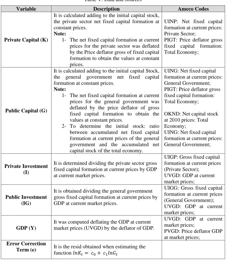
Table V: Data and Sources

Variable Description Ameco Codes

Private Capital (K)

It is calculated adding to the initial capital stock, the private sector net fixed capital formation at constant prices.

Note:

1- The net fixed capital formation at current prices for the private sector was deflated by the Price deflator gross of fixed capital formation to obtain the values at constant prices.

UINP: Net fixed capital formation at current prices: Private Sector;

PIGT: Price deflator gross fixed capital formation: Total Economy;

Public Capital (G)

It is calculated adding to the initial capital Stock, the general government net fixed capital formation at constant prices.

Note:

1- The net fixed capital formation at current prices for the general government was deflated by the price deflator of gross fixed capital formation to obtain the values at constant prices.

2- To determine the initial stock: ratio between accumulated net fixed capital formation at current prices of the general government and the accumulated net capital stock of the total economy.

UING: Net fixed capital formation at current prices: General Government; PIGT: Price deflator gross fixed capital formation: Total Economy;

OKND: Net capital stock at 2010 prices: Total Economy;

UING: Net fixed capital formation at current prices: General Government;

Private Investment (I)

It is determined dividing the private sector gross fixed capital formation at current prices by GDP at current market prices.

UIGP: Gross fixed capital formation at current prices (Private Sector);

UVGD: GDP at current market prices;

Public Investment (IG)

It is obtained dividing the general government gross fixed capital formation at current prices by GDP at current market prices.

UIGG: Gross fixed capital formation at current prices (General Government); UVGD: GDP at current market prices;

GDP (Y)

It was computed deflating the GDP at current market prices (UVGD) by the deflator of GDP.

UVGD: GDP at current market prices;

PVGD: Price deflator GDP at market prices;

Error Correction

Term (e) It is the resid obtained when estimating the

(28)

20

Table VI: Statistic Information I

Private Capital (K) Public Capital (G) Private Investment (I) Public Investment (IG) GDP (Y) Error Correction Term (e) Mean 355.9731 38.67356 0.200828 0.038870 145.5907 -3.99E-17 Median 367.2538 40.07556 0.198349 0.040769 161.0457 -0.017065 Maximum 472.0235 73.73249 0.275784 0.055683 184.2624 0.290932 Minimum 184.4059 0.963449 0.125806 0.015484 87.16390 -0.065447 Std. Dev 100.5614 26.18507 0.041941 0.010575 33.71893 0.063636 For the above computations, no natural logarithms were applied to the data.

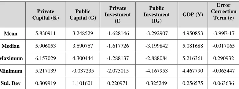
Table VII: Statistic Information II

Private Capital (K) Public Capital (G) Private Investment (I) Public Investment (IG) GDP (Y) Error Correction Term (e) Mean 5.830911 3.248529 -1.628146 -3.292907 4.950853 -3.99E-17 Median 5.906053 3.690767 -1.617726 -3.199842 5.081688 -0.017065 Maximum 6.157029 4.300444 -1.288137 -2.888084 5.216361 0.290932 Minimum 5.217139 -0.037235 -2.073015 -4.167953 4.467790 -0.065447 Std. Dev 0.309919 1.101601 0.220971 0.325249 0.256575 0.063636 For the above computation, natural logarithms were applied to the data, except to the error correction

(29)

21

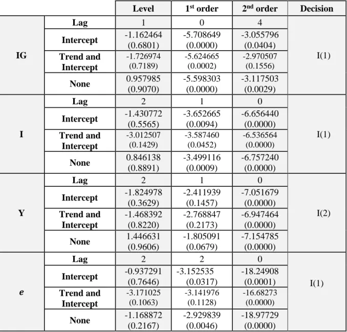
Table VIII: ADF Test of the other variables

Level 1st_order ₂nd_order _Decision

IG Lag 1 0 4 I(1) Intercept -1.162464 (0.6801) -5.708649 (0.0000) -3.055796 (0.0404) Trend and Intercept -1.726974 (0.7189) -5.624665 (0.0002) -2.970507 (0.1556) None 0.957985 (0.9070) -5.598303 (0.0000) -3.117503 (0.0029) I Lag 2 1 0 I(1) Intercept -1.430772 (0.5565) -3.652665 (0.0094) -6.656440 (0.0000) Trend and Intercept -3.012507 (0.1429) -3.587460 (0.0452) -6.536564 (0.0000) None 0.846138 (0.8891) -3.499116 (0.0009) -6.757240 (0.0000) Y Lag 2 1 0 I(2) Intercept -1.824978 (0.3629) -2.411939 (0.1457) -7.051679 (0.0000) Trend and Intercept -1.468392 (0.8220) -2.768847 (0.2173) -6.947464 (0.0000) None 1.446631 (0.9606) -1.805091 (0.0679) -7.154785 (0.0000) 𝒆 Lag 2 2 0 I(1) Intercept -0.937291 (0.7646) -3.152535 (0.0317) -18.24908 (0.0001) Trend and Intercept -3.171025 (0.1063) -3.141976 (0.1128) -16.68273 (0.0000) None -1.168872 (0.2167) -2.929839 (0.0046) -18.97729 (0.0000)

(Note) The sample considered is from 1980 to 2018. Schwarz Information Criterion was used for the lag selection. The entries are the test statistics. The values in parentheses are the p-values. The variables are: private investment (I), public investment (IG), GDP (Y) and the error correction term (e).

(30)

22

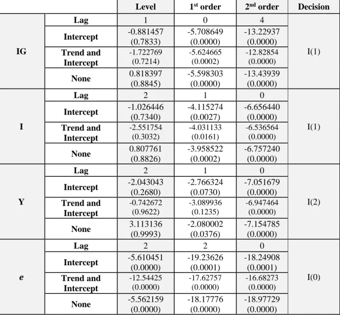
Table IX: PP Test of the other variables

Level 1st_order ₂nd_order _Decision

IG Lag 1 0 4 I(1) Intercept -0.881457 (0.7833) -5.708649 (0.0000) -13.22937 (0.0000) Trend and Intercept -1.722769 (0.7214) -5.624665 (0.0002) -12.82854 (0.0000) None 0.818397 (0.8845) -5.598303 (0.0000) -13.43939 (0.0000) I Lag 2 1 0 I(1) Intercept -1.026446 (0.7340) -4.115274 (0.0027) -6.656440 (0.0000) Trend and Intercept -2.551754 (0.3032) -4.031133 (0.0161) -6.536564 (0.0000) None 0.807761 (0.8826) -3.958522 (0.0002) -6.757240 (0.0000) Y Lag 2 1 0 I(2) Intercept -2.043043 (0.2680) -2.766324 (0.0730) -7.051679 (0.0000) Trend and Intercept -0.742672 (0.9622) -3.089936 (0.1235) -6.947464 (0.0000) None 3.113136 (0.9993) -2.080002 (0.0376) -7.154785 (0.0000) 𝒆 Lag 2 2 0 I(0) Intercept -5.610451 (0.0000) -19.23626 (0.0001) -18.24908 (0.0001) Trend and Intercept -12.54425 (0.0000) -17.62757 (0.0000) -16.68273 (0.0000) None -5.562159 (0.0000) -18.17776 (0.0000) -18.97729 (0.0000)

(Note) The sample considered is from 1980 to 2018. Schwarz Information Criterion was used for the lag selection. The entries are the test statistics. The values in parentheses are the p-values. The variables are: private investment (I), public investment (IG), GDP (Y) and the error correction term (e).