THE CAUSAL RELATIONSHIP BETWEEN TAXES AND EXPENDITURES IN PORTUGAL: COINTEGRATION AND ERROR-CORRECTION MODELS

Esruoos DE EcoNOMIA, VOL. XVIII, N.0 _{1, INVERNO 1997}

THE CAUSAL RELATIONSHIP BETWEEN TAXES

AND EXPENDITURES IN PORTUGAL:

COINTEGRATION AND ERROR-CORRECTION MODELS

Antonio Luis Silvestre

(*)

1 - Introduction

The reduction of fiscal deficit is one of the purposes of Portuguese gov-ernment in order to achieve the convergence criterion on deficits for participa-tion of Portugal in the European Monetary Union (EMU). However, the reduc-tion of the deficit may be achieved either by increasing taxes or decreasing expenditures or both. But if taxes cause expenditures, an increase in taxes implies an increase in expenditures and the deficit may incidently increase. If expendi-tures cause taxes, a cut in expendiexpendi-tures induces a cut in taxes and again the deficit may not reduce. Hence, the existence and direction of causality between expenditures and revenues is an important issue.

Recently, a number of studies have investigated the causal relationship between government expenditures and tax revenues for several countries. For example, the studies of Anderson et al. (1986), Ram (1988a), Joulfaian and Mookerjee (1990a) and Manage and Marlow (1986) for the United States, and for other countries, Ram (1988b) for a group of 22 countries including devel-oped and developing countries, Joulfaian and Mookerjee (1990b) for 17 OECD countries, Baffes and Shah (1994) for three Latin American countries (Argen-tina, Brazil and Mexico), and Owye (1995) for the most developed countries (G7 group).

These papers use different methodologies and different types of data. With respect to the methodology, most studies use the conventional Granger-Sims causality tests but others use most recent developments of the econometric techniques, namely, cointegration and error-correction models.

In the present paper we apply the cointegration and error-correction meth-odology to examine the causal relationship between government expenditures and government tax revenues in Portugal over the period 1958-1991.

The rest of the paper is organized as follows. Section 2 presents a review of the relevant literature, section 3 describes the econometric methodology and section 4 presents the data.and discusses the empirical results. Finally, section 5 summarizes and concludes the paper.

2 - Literature review

Three main hypotheses or theories on the direction of the causality between government expenditures and government revenues may be

ESTUDOS DE EcoNOMIA, VOL. XVIII, N.0 _{1, fNVERNO 1997}

postulated: the first states there is a bidirectional causal relationship; according to the second, revenues (taxes) may lead government spending; and the third advocates that spending may lead taxes.

According to the first theory, expenditures and taxes are decided by the governments jointly. This is the case often referred in textbooks on Public Eco-nomics [see, for example, Musgrave (1966) and Meltzer and Richard (1981)]. The second hypothesis, expenditures adjust to taxes is consistent with the lit-erature on state and local finances and finds also support among supply-side economists. These authors argue that increases in taxes only result in increased expenditures and not in deficit reduction [see Roberts (1984)]. The third situa-tion occurs when taxes adjust to expenditures and was explored in Peacock and Wiseman (1979). These authors found that temporary changes in govern-ment spending lead to permanent changes in taxes.

There is yet a fourth possibility: absence of causal relationship between expenditures and taxes. According to this hypothesis, expenditures and taxes are decided in a independent causal way.

The fundamental question is: which of these hypotheses is supported for each country or for each group of countries? The analysis in the literature is conducted at state or local level as well as at the federal level. The most stud-ies on causality between expenditures and taxes are concerned with the U. 8. However, there are some studies for other countries, including developed and least developed countries. The findings of these studies are mixed. For Portu-gal, as far as we know, Joulfaian and Mookerjee (1990b) is the only work where the issue of causality between government expenditures and taxes is studied. The results of this study concerning Portugal support the tax-and-spend hypoth-esis:

Overall, the results suggest that the tax-and-spend hypothesis seems more relevant in the U. 8., Canada, and Portugal, and the spend-and-tax hypothesis in countries such as Japan, the United King-dom, France and Greece, Ireland, and the Netherlands. [Joulfaian and Mookerjee (1990b), page 112.]

The evidence on the relevance of the above four hypotheses is mixed in current literature. For example, for the United States, Manage and Marlow (1986) have found some evidence of a unidirectional relationship from revenues to ex-penditures while von Furstenberg et al. (1985, 1986) and Anderson et al. (1986) found support for the causality in the opposite direction, that is, the spend-and-tax hypothesis. According to the results of the latter authors, spending increases lead to tax increases and not vice-versa.

Esruoos DE EcoNOMIA, VOL. XVI/I, N.0 _{1, INVERNO 1997} Consumer Price Index (CPI), the implicit GNP deflator, and the implicit deflator for the federal or the state-local government sector. His major conclusion is the following:

There is considerable variation in the results for different cases. In general, however, it seems that causality runs mainly from revenue to expenditure in the federal data, but predominantly from expenditure to revenue in data for the state and local government sector. [Ram (1988a), page 763.]

Ram (1988b) investigates the causal relationship between government ex-penditures and revenues for a group of 22 countries including developed coun-tries (DC) and least developed councoun-tries (LDC). His results are mixed:

The most significant aspect is that there is much cross-country variation in the causal patterns and it is hazardous to draw general conclusions. Along with the lack of a significant causal flow in most cases, one can find practically any causal pattern by selecting a suit-able subset of countries. [Ram (1988b), page 263.]

With respect to the state of development of the countries he concludes «there is no discernible difference between the results for the DCs and the LDCs» and with respect to nominal or real data, there is almost as many cases of causality from revenue to expenditures as of causal flow in the opposite direc-tion for nominal data and for real data, «[ ... ] when one does observe a signifi-cant causal order, causality seems to run more frequently from revenue to ex-penditure» [Ram (1988b), page 263].

Miller and Russek (1990) apply cointegration and error-correction models to examine the causal relationship between tax revenues and expenditures for the U.S. They show how sources of causality can be neglected in standard Granger causality tests. They use quarterly data and their results suggest bidi-rectional causality between government taxes and expenditures, both for the fed-eral, and state and local levels.

Baffes and Shah (1994), besides the examination of the causality relation-ship between expenditures and taxes, test also the stationarity hypothesis of fiscal deficits for Argentina, Brazil, and Mexico. They use cointegration and error-cor-rection models for the causality tests, the fiscal deficit being the error-corerror-cor-rection term for the countries where the deficits were stationary. Their findings suggest that deficits were stationary in Argentina and Mexico but not in Brazil. Regard-ing the direction of causality, they found bidirectional causality for Argentina and Mexico and unidirectional causality running from revenues to expenditures for Brazil.

Esruoos DE EcoNOMIA, voL. xvm, N.O 1, INVERNO 1997

3 - Econometric methodology

In this paper, besides the standard Granger c·ausality test, we use cointegration and error-correction modelling to investigate the causal linkage between government expenditures and tax revenues. Since cointegration is applied to nonstationary time series and the standard Granger causality tests and the error-correction modelling require stationary series, the econometric methodology follows in three steps. In the first, the properties of the time series are studied. Unit roots tests are performed for determination of the order of in-tegration of the series.

In the second step, the series are tested for cointegration, and in the third step, an error-correction model is estimated and used for testing the existence of causality between government expenditures and government tax revenues.

3.1 - Unit root tests

The unit root tests we apply are the Dickey-Fuller (OF), the Augmented Dickey-Fuller (ADF) tests [Dickey and Fuller (1979, 1981 )] and the test suggested by Phillips (1987) and Phillips and Perron (1988). The latter is more robust than the ADF test in the cases where there is autocorrelation or heteroscedasticity. These tests are performed to determine the series order of integration. The order of integration of a series is the number of times a series need to be differenced to achieve stationarity. The tests are implemented in the fol-lowing way.

Let denote a particular series by y₁ (t= 1 ,2, ... , T). The Dickey-Fuller (OF) test is based on the estimation of one of the following two equations:

(1)

(2)

where £

11 and ~~ are the assumed uncorrelated error terms of the equations. In

the second equation a time trend is considered while in the first equation it is not. The null hypothesis H₀ states that the series has a unit root (i. e., the se-ries is nonstationary). Formally, the null hypothesis H₀ is a₁

=

0 or ~

=

0 ac-cording to the equation considered. For testing the null hypothesis we compute the t-statistic in the usual way but the distribution of this statistic is nonstandard. Critical values were supplied by Dickey and Fuller (1979, 1981 ). If

H

₀ is rejected, the series y₁ is stationary and if

H

₀ is not rejected the series is nonstationary. For those series which are nonstationary differencing is needed.

If the error terms are correlated, lagged values of the dependent variable are added until the errors are noncorrelated and we have then the Augmented Dickey-Fuller (ADF) test.

EsTUDOS DE ECONOMIA, VOL. XVIII, N.' 1, /NVERNO 1997 The tests are performed on the basis of the estimation of one of the fol-lowing two auto-regressive equations:

k

~Yt

= J..l1 + 0:1 Yt-1 +

L

0i

~Yt-i

+ £11 i=1

k

~Yt = ~ + ~t + 0:2Yt-1 +

L

'Yi ~Yt-i + ~~

i=1

(3)

(4)

In the practice, we follow a sequence of tests [see Dickey and Fuller (1981), page 1 070, table x]:

1) H₀ : o:₂ = 0;

2)

Ha

:

o:2

=

~

=

J..l2

=

0; 3)

H

₀ : o:₂

=

~

=

0; 4) H₀ : o:₁ = 0;

5)

Ha

:

o:1

=

J..l1

=

0.

These tests are performed until all test statistics are significant. If we could not reject the null hypothesis, the series is nonsationary in levels. DF, ADF and the PP test of Phillips and Perron are then performed on the series of first dif-ferences. If the null of a unit root is rejected, the series in differences is station-ary and thus the series in levels is 1(1). If the null hypothesis is not rejected, the series of the first differences is nonstationary and one performs DF, ADF and the PP tests on the second differences and so on. The order of integration of a time series is the number of times a series must be differenced for achieving stationarity.

3.2 - Cointegration tests

With respect to cointegration tests, two types of cointegration tests are applied: the Engle-Granger test and the Johansen test.

The cointegration tests require that both variables under consideration are of the same order of integration. Two series integrated of order one are cointegrated if both have a common trend, that is, if there is a linear combina-tion of them which is stacombina-tionary. In the case of cointegracombina-tion, the two series can not drift apart one from the other. The second step is thus to test whether the two series are cointegrated.

Let us first describe the Engle-Granger cointegration test and then the Johansen's maximum likelihood test of cointegration.

Let denote the two time series by y₁ and

x

₁ (in the application these series are the growth rates of government expenditures and tax revenues, respectively). The Engle-Granger cointegration test is based on the OLS residuals of the fol-lowing cointegration equations:

Yt= a+ ~xt+ ut

I A' xt = o: + ~-' Yt + vt

where

u

₁ and

v

₁ stand for the error terms of the equation regressions.

(5)

Esruoos DE EcoNOMIA, VOL. xvm, N. o 1, INVERNO 1997

The null hypothesis of the Engle-Granger cointegration test is that the two variables 1(1) are not cointegrated. If the variables are not cointegrated the residuals

u

₁ and

v

₁ are not stationary. Therefore, the cointegration test is a unit root test of the series of residuals.

The Johansen's likelihood test is applied in the following way. Suppose that the data-generating process for a vector

z

₁ of N 1(1) variables may be written as an mth-order vector autoregression (VAR):

where 11₁ is independent mean 0 with a constant variance.

This equation may be rewritten as:

where

l;= -/

+

n1

+ ... + ll;(1

=

1,2, ... ,m) and

r

m =-1-

n1- ... - nm.

The test is a test on the rank of the matrix

r

m. The rank of this matrix determines the number of distinct cointegrating vectors which exist between the

variables in

z.

Thus, if

r

m has rank of 0, then the null hypothesis of no

cointegration cannot be rejected.

Defining two N x r matrices a and ~ such that:

im=aW

the rows of

W

form r distinct cointegrating vectors such that, if ~; is the

i

1h row of

W:

Johansen (1988) demonstrates that the likelihood ratio (LR) test statistic

for the hypothesis that there are at most r distinct cointegrating vectors is:

N

LR=- T

L

ln(1-1;)

i= r+1

where

1r+

_{1, ...}

,1N

are the N-r smallest square canonical correlations between

the

z

₁_k and llz₁ series, corrected for the effect of the lagged differences of the

z

process [for details of how to extract the \ see Johansen (1988, 1991 )].

Johansen (1988) shows that LR will have a non-standard distribution under the

null hypothesis. He does, however, provide approximate critical values for this statistic, generated by Monte Carlo methods.

Esruoos Do EcoNOMtA, VOL. xvm, N.0 _{1, INVoRNo 1997}

3.3 - Causality tests

In the literature on causality there are several tests for testing the exist-ence of a causal relationship between two variables.

One of these tests is Granger's (1969) direct test based on his definition of causality. According to this definition,

y

causes x if the past values of

y

im-prove the prediction of

x.

This is the standard Granger causality test and

re-quires stationary variables. The test is performed in the following way.

Assuming that the variables in levels are integrated of order one, 1(1 ), the series of the first differences are 1(0). Therefore, the test is based on the two following equation regressions:

m n

-1Yr = a1 + L

~1i-1Yr-i

+ LY1j.1xt-j + Er (7)

i= 1 j=1

n m

Mr = a2 +

L

Y2i.1xt-i +

L

~2i-1Yr-i

+ llr (8)

j=1 i=1

The small sample properties of this test and the test proposed by Sims (1972) and a modified Sims test suggested by Geweke et al. (1983) were stud-ied by Guilkey and Salemi (1982). These authors concluded that «the Granger test performs slightly but significantly better than the other tests» (page 673). Moreover, «since the Granger test is computationally the least expensive of the three and results in the fewest degrees of freedom lost from formation of lags and leads••, the authors «recommend it confidently to the practitioner» [Guilkey and Salemi (1982), page 679]. According to the authors, for sample size less than 200 the shorter versions of all three tests are superior to the longer versions. For these reasons, the causality tests we use in this paper are of Granger type.

However, a more comprehensive test of causality was provided by Granger (1983,1986) and Engle and Granger (1987). This new causality test applies cointegration and error-correction methodology and allows for a causal linkage between two variables stemming from a common trend or equilibrium relation-ship. If two variables have a common trend, that is, are cointegrated, the lagged level of one of the variables may help to explain the current change in an-other variable, even if past changes of the former do not. This causality may not be detected by the standard Granger causality test [see Miller and Russek (1990)].

For testing causality by applying the error-correction methodology, we add the error-correction term (ECT) to the regression equations 7 and 8. This ECT is the estimated OLS residuals of the cointegration equations (eq. 5 and eq. 6) with one lag:

m n

.1yt = a1 +

L

~1i-1Yr-i + LY1i.1xt-i + 01 [jr-1 + £1 t (9)

i= 1 j= 1

n m

.1xt

=

a2 + LY2i.1xt-i +

L

~2i-1Yt-i + 02 vt-1 + £21 (10)

E5TUD05 DE ECONOMIA, VOL. XVIII, N.0 _{1, INVERNO 1997}

The null hypothesis «X does not causeY'' is H₀: y₁j= 0; j= 1,2, ... ,n; 8₁ = 0. If this hypothesis is rejected there is a causal relationship running from x to

y;

otherwise, there is not a causal relationship in this direction. The null for testing a unidirectional relationship in the opposite direction is H₀ : ~

2

i = 0;

i

= 1 ,2, ... ,m; 8₂ = 0. The rejection of this hypothesis implies there is a one way causal link from y to x. If both hypotheses are jointly rejected there is a bidirectional rela-tionship between expenditures and taxes and, finally, if both hypothesis are not rejected, there is no causal relationship between the two variables. If 8₁ or 8₂ or both are significant then the linkage from long run equilibrium relationship is an important one.

A major concern in performing a causality test is the order of lags among the variables. Some authors use an arbitrary number of lags. The numbers 1, 2, 3 and 4 are common numbers used for annual data. But, as pointed out by Thornton and Batten (1985), an arbitrary number of lags may produce mislead-ing results. An alternative is to use some criterion for the selection of model specification. These authors use three different criteria for specifying the lag length: Akaike's (1970) final prediction error (FPE) suggested by Hsiao (1981 ), Bayesian estimation criterion (BEG) suggested by Geweke and Meese (1981), and a criterion suggested by Pagano and Hartley (1981). Their results «suggest that the arbitrary lag-length specifications fail to ensure that the results are not based on the capricious choice of the lag-structure» [Thornton and Batten (1985), page 176]. They recommend also that «the safest approach is to perform an extensive search of the lag space» but «even when this approach is taken, how-ever, care must be taken in interpreting the results» (page 177).

According to these authors, among the criteria they considered, the Akaike's FPE criterion is the one suggested. «A comparison of several commonly used criteria for lag-length selection suggests that based on standard, classical, hy-pothesis-testing norm AKAIKE's FPE criterion performed well in selecting the model relative to the others. As a result, it did a reasonably good job of finding an order of the model which gave evidence of Granger causality, when such an order existed» [Thornton and Batten (1985), page 177].

Following Akaike's formulation of the FPE(m, n) estimate, a two step

ap-proach to find the lags values of m and n may be used. First, one selects the

value of

m

(n) which minimizes FPE when regressing ~y

₁

(&₁) on its own lags. Given that

m

(n) value, the lag values of & (~y) are included in the equation to

choose the

n

(m) value which yields the FPE minimum. Finally, based on these

values of m. and

n,

we test the null hypothesis that the coefficients of the lags of & (~y) are jointly zero. However, in the application below we have used a

different approach. Although the values of m and n need not be equal, for the

sake of simplicity in ttie computations, we have taken

m =

n

and minimized FPE

(m + n) for

m

=

n

=

1 ,2,3,4.

Esruoos DE EcoNOMIA, VOL. XVIII, N.0 _{1, INVERNO 1997}

4 - Data and empirical results

The data concern current government expenditures and current tax rev-enues at current prices (nominal data). The data were obtained from Santos et al. ( 1992} and cover the period 1958-1991.

Some authors argue that nominal data is more appropriate than real data since the decisions on expenditures and revenues are undertaken at a nominal level. Following these authors, we do not deflate expenditures and tax revenues with a price index thus considering the data at current prices. However, the de-cisions on taxes and spending are sometimes undertaken as a proportion or percentage of GOP and we could «deflate» the data using as deflator the GOP (actual or potential) as Von Furstenberg et al. (1986) or Hoover and Sheffrin (1992} do.

We have only considered current expenditures and revenues and not total expenditures and total tax revenues because capital expenditures and capital receipts have had a very different behavior in the period covered by the analy-sis. Total expenditures and total tax revenues as a percentage of GOP will be considered in a future paper.

The time series in natural logarithms of levels are depicted in figure 1 and the first differences (growth rates) in figure 2. These pictures show evidence of nonstationarity of both series in levels and in growth rates.

The second differences of the logarithms of expenditures and revenues (changes of growth rates) are presented in figure 3. According to this graph, second differences seem to be stationary. Thus, the two series appear to be integrated of order two, that is, 1(2}.

FIGURE 1

Current government expenditures and revenues (in logs)

15.2482

13.2260

Log( expenditures)--Log(revenues)

1976

.··

.•..• ··

.---···/

Esruoos D£ EcoNOMIA, voL. XVIII, N.0 _{1, /NVERNO 1997}

FIGURE 2

Current government expenditures and revenues growth rates

.33803

.23937

.11071

.042047 /

1~9~5~8~~~~~~~~~~~~~1~9=7 76~~~~~~1~9~85~~~~19~91

Expenditures -Revenues

FIGURE 3

Changes of growth rates of government expenditures and revenues

. 1 5 1 9 4 r - - - . - - - .

.051632

~~

I

-.848680

-.14899~~~~~~~~~~~~~~~--~~--~~~~~

1958 1967 1976 1985 1991

Esruoos DE EcoNOMtA, voL. xvm, N.• 1, /NVERNo 1997

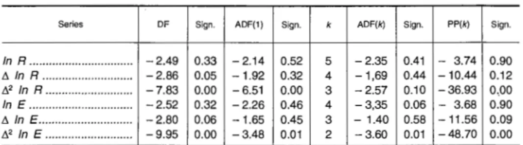
Below, we apply formal tests for the determination of the order of integra-tion of the series. First, we apply the DF, ADF and the PP tests to the series and conclude that tax revenues and expenditures (in logs) are nonstationary se-ries. The application of these tests to the first differences (growth rates) shows that the growth rates of the two time series are also nonstationary. Finally, the null hypothesis of nonstationarity of the second differences is rejected. There-fore, the expenditures and tax revenues series are both integrated of order two, 1(2), the first differences (growth rates) being integrated of order one, 1(1 ).

Table 1 reports the results of the DF, ADF and PP tests for the levels of the variables, for the first differences and for the second differences:

TABLE 1

Results of DF, ADF and PP unit root tests

Series DF Sign. ADF(1) Sign. k ADF(k) Sign. PP(k) Sign.

In R ... -2.49 0.33 -2.14 0.52 5 -2.35 0.41 - 3.74 0.90

L1 In R ... -2.86 0.05 -1.92 0.32 4 -1,69 0.44 -10.44 0.12

L}2 _{In R ... -7.83 0.00 -6.51 0.00 3 -2.57 0.10 -36.93 0 .. 00}

In E ... -2.52 0.32 -2.26 0.46 4 -3,35 0.06 - 3.68 0.90

L1 In E ... -2.80 0.06 -1.65 0.45 3 - 1.40 0.58 - 11.56 0.09

L}2 _{In E ... -9.95 0.00 -3.48 0.01 2 -3.60 0.01 -48.70 0.00}

Notes.- In R =tax revenues (in logs); In E =expenditures (in logs); k is the optimal number

of lags according to the AIC (Akaike Information Criterion) criterion; L11n R and L1 In E are the

growth rates of tax revenues and expenditures, respectively, and .12 _{In R and .1}2 _{In E are the}

changes of growth rates of tax revenues and expenditures, respectively; the Lagrange Multiplier (LM) statistic for testing first order autocorrelation of the errors corresponding to ADF(1) is not significant for all series.

According to the results of this table, the variables in levels and in growth rates (first differences) are not stationary. However, the second differences are stationary, 1(0). Thus, in nominal values, currrent government expenditures and currrent government revenues are integrated of order two, 1(2).

This result is not very usual in the literature on this subject. In general, the series are either supposed (implicitly) integrated of order one by some authors which do not study the properties of the series but use the first differences of the series (in general in logarithms) or the reported results on stationarity do not reject the hypothesis that the series are integrated of order one.

Esruoos DE EcoNOMIA, voL. XVIII, N." 1, INVERNO 1997

are also integrated of order two as is the case of (current) expenditures and (currrent) taxes in Portugal over the period considered.

Like most authors in this area, in what follows we consider the variables in growth rates. Thus, the variables are in natural logarithms converted to growth rates by taking the first differences. Use of growth rates is consistent with fiscal budgetary exercises that are generally undertaken in terms of growth rates and is convenient for the cointegration issue.

In fact, the Engle-Granger cointegration test for two time series requires that both series are integrated of order one, 1(1 ), since the null hypothesis is that the series of residuals has a unit root and the alternative is that the series is stationary, 1(0). Thus, in the cointegration equation regressions, we consider the series of the first differences (growth rates) of government expenditures and tax revenues, denoted by y₁ and

x

₁, respectively.

The results of the cointegration tests (OF and ADF) are reported in Ta-ble 2. As one may see in this taTa-ble, the null hypothesis

H

₀, the series of residuals have a unit root, is rejected at the 1 0 % significance level when we use the OF and the ADF(1) tests. The null is not rejected if we consider the optimal lag given by the AIC criterion. However, the LM statistic for testing autocorrelation of the errors of the equation corresponding to the OF or ADF(1) statistics is not significant. Thus, we may consider that the variables (growth rates of expendi-tures and tax revenues) are cointegrated.

TABLE 2

Cointegration equations and OF and ADF unit root tests for OLS residuals

Coefficients of Test statistics

Oep. var.

Canst. x, Y, ow OF Sig. AOF(1) Sig. k AOF(k) Sig.

y, ... .02 .94 - 1 1.8o -4.35 .00 -3.19 .07 2 -2.75 .18

x, ... .04 - .72 i 1.64 -4.61 .00 -4.02 .01 4 -2.55 .26

Note. -The LM statistics for testing autocorrelation corresponding to the DF and ADF(1)

are not significant at the 5 % level of significance; k is the optimal lag according to the AIC criterion.

The same conclusion is drawn from the cointegration residuals Durbin Watson (CROW) test. The null hypothesis of this test is rejected for high values

of OW. The high values of the Durbin Watson statistics show evidence of

sta-tionary residuals and thus of cointegrated variables.

However, we also apply the Johansen's Likelihood Ratio (LR) test to the growth rates of government expenditures and revenues. The results of this test are reported in Table 3. We conclude again that the variables are cointegrated, the cointegrating vector beeing (-1 0. 79).

Esruoos DE EcoNOMIA, VOL. XVIII, N.0 _{1, INVERNO 1997}

Null

r= 0

r$1

TABLE 3

Results of the LR cointegration tests of Johansen (Maximal Eigenvalue and Trace tests)

Maximal Eigenvalue test Trace test

Altern. Stat. Grit. val. Null Altern.

r= 1 20.94 14.90 r= 0 r;:: 1

r=2 3.04 8.18 r$1 r=2

Stat. Grit. val.

23.98 17.95

3.04 8.18

Notes.-The maximum lag in the VAR is optimal according to the AIC criterion and is equal to 2; the critical value corresponds to the 5 % level of significance.

Since the variables are cointegrated, we know from Engle and Granger (1987) that there is at least a unidirectional causal relationship between the variables. For testing the existence of a causal link, we first apply the standard Granger causality test. The results are reported in Table 4 and show evidence of a causal relationship running from expenditures to tax revenues.

TABLE 4

Results of the standard Granger causality test

lndep. variables

Constant ... ..

t.y,_, ·-····-··-··-···-···-···-·-···

t.y,_2 -···--···--···-·-···-··-··'"'"''''''''

t.y,_3 ... .

t.x,_, ···-···

t.x,_2 ... .

t.x,_3

···-···-···-··-···-··-Diagnostic statistics:

Expeditures equation Dependent variable fly,

Revenues equation Dependent variable llx,

Coeff. T-statistic Sig. level Coeff. T-statistic Sig. level

.006 .564

- .642 - 3.602

.119 .520

.577 .001 .607 .008 .106 .614 .369 - .811 -.897 -.324

.956 .350 .639 .530 3.250 .004 2.052 .052 -3.464 .002 -4.016 .001 -1.379 .182

Expenditures equation: R2

=

.315; DW

=

1.800; F(2,28)

=

7.885 (.002); SER

=

.063; LM(1)

=

.209 (.647); LR(1)

=

.298 (.585);

Revenues equation: R2

=

.497; DW

=

1.907; F(6,22)

=

5.615 (.001 ); SER

=

.043; LM(1) = .003 (.956); LR(3) = 13.378

(.004)-Notes. - LM(p) is the Lagrange Multiplier statistic for testing error serial correlation of order

p which has an asymptotic chi-square distribution with p degrees of freedom and in parentheses is the significance level; SER is the Standard Error of Regression ; LR(k) is the Likelihood Ratio statistic for joint test of zero restrictions on the coefficients of the k deleted variables.

Esruoos DE EcoNOMIA, VOL. xvm, N.0 _{1, INVERNO 1997}

TABLE 5

Results of the error-correction models tests of causality

lndep. variables

Constant ... .. L'ly,_, ... . L'ly,_2 ... . L'lx,_, ... .

~x,_2 ··-··· .. ···-··· .. ..

·-u,_, ... .

v,_,

-·-····-·"--··---···---· .. ··-·· .. ···--··-·-··--"'

Diagnostic statistics:

Expeditures equation Dependent variable t.y,

Revenues equation Dependent variable t.x,

Coeff. T-statistic Sig. level Coeff. T-statistic Sig. level

.006 .507

-.516 -2.112

.014 .053

-.250 .762

.616 .044

.958

.453

.011

I

-.499

.061 -.039 -.420

-.966

1.502 .146 -2.201 .038 .338 .738 - .169 .867 -2.346 .028

-3.018 .006

Expenditures equation:

R

2

₌

_{.304; DW}

₌

_{1.740; F(3,27)}

₌

_{5.371 {.005); SER}

₌

_.063; LM(1)

=

.854 (.355); LR(2)

=

.957 (.620);

Revenues equation:

fl2

=

.557; DW

=

2.243; F(5,24)

=

8.904 (.000); SER

=

.039; LM(1) = 2.244 (.134); LR(3) = 17.678 (.001).

Notes. - LM(p) is the Lagrange Multiplier statistic for testing error serial correlation of order

p which has an asymptotic chi-square distribution with p degrees of freedom and in parentheses is the significance level; SER is the Standard Error of Regression ; LR(k) is the Likelihood Ratio statistic for joint test of zero restrictions on the coefficients of the k deleted variables.

From the results in this table we conclude again that there is causality from expenditures to tax revenues and that the link due to the long run equilibrium relationship is important In sum, we concluded that a unidirectional causal rela-tionship exists running from the expenditures to the revenues. Thus, the hypoth-esis of spend-and-tax seems to be verified tor Portugal over the period 1958-1991, a result in opposition to the findings of Joultaian and Mookerjee (1990b) tor PortugaL

5 - Summary and conclusions

This paper investigated the causal relationship between government expen-ditures and tax revenues tor Portugal over the period 1958-1991. The data used concern current expenditures and current tax revenues at current prices (nomi-nal data). Data were converted to growth rates by considering the first differ-ences of natural logarithms.

The methodology applied is the recent cointegration and error-correction modelling which provides additional channels through which causality could emerge.

Esruoos DE EcoNOMIA, voL. xvm, N.0 _{1, INVERNO 1997}

but the changes of the growth rates are stationary. Hence, growth rates are integrated of order one, 1(1 ), the series in levels being 1(2).

The results of the Engle-Granger and Johansen tests of cointegration showed that the growth rates of the two variables are cointegrated. Hence, a causal relationship between government expenditures and tax revenues exists at least in one direction.

The estimation of an error-correction model showed that the causal rela-tionship runs from expenditures to tax revenues and the additional causality channel referred above is significant.

Esruoos DE EcoNOMIA, VOL. xvm, N.0 _{1, INVERNO 1997}

REFERENCES

AHIAKPOR, J. C., and AMIRKHALKHALI, S. (1989), «On the Difficulty of Eliminating Deficits with Higher Taxes», Southern Economic Journal, 56, pp. 24-31.

AKAIKE, H. (1969),«Fitting Autoregressions for Prediction», Annals of the Institute of Statistical

Mathematics, 21, pp. 243-47.

- - (1970)] , «Statistical Predictor Identification», Annals of the Institute of Statistical

Mathemat-ics, 22, pp. 203-17.

ANDERSON, W., WALLACE, M. S., and, WARNER, J. T. (1986), «Government Spending and Taxation: What Causes What?» Southern Economic Journal, 52, pp. 630-639.

BAFFES, J., and SHAH, A. (1994), «Causality and Comovement between Taxes and Expendi-tures: Historical Evidence from Argentina, Brazil, and Mexico», Journal of Development

Eco-nomics, vol. 44, pp. 311-331.

SARRO, Robert J. (1979), «On the Determination of the Public Debt,» Journal of Political Economy,

81 (Oct.), pp. 940-971.

BLACKLEY, P. R. (1986), «Causality Between Revenues and Expenditures and the Size of the Federal Budget», Public Finance Quarterly, vol. 14, no. 2, pp. 139-56.

DICKEY, D., and FULLER, W. (1979), «Distribution of Estimates of Autoregressive Time Series with Unit Root», Journal of the American Statistical Association, 74, pp. 27-31.

--(1981), «The Likelihood Ratio Statistics for Autoregressive Time Series with a Unit Root»,

Econometrica, 49, pp. 1057-72.

ENGLE, Robert F., and GRANGER, C. W. J. (1987), «Co-Integration and Error Correction: Repre-sentation, Estimation, and Testing.» Econometrica, March, pp. 251-76.

ENGLE, R. F., and YOO, B.S. (1987), «Forecasting and Testing in Co-Integrated Systems», Journal

of Econometrics, 35, pp. 143-159.

FULLER, Wayne A. (1976), Introduction to Statistical Time Series, New York, Wiley.

FURSTENBERG, George von (1983), «Fiscal Deficits: From Business as Usual to a Breach of the Policy Rules?» National Tax Journal, 36, Dec., pp. 443-457.

FURSTENBERG, George von, GREEN, R. Jeffrey, and JEONG, Jin-Ho (1985), «Have Taxes Led Government Expenditures? The United States as a Test Case», Journal of Public Policy,

vol. v, no. 3, pp. 321-48.

- - (1986), «Tax and Spend, or Spend and Tax?», Review of Economics and Statistics, vol. 68, pp. 179-88.

GEWEKE, J., and MEESE, R. (1981), «Estimating Regression Models of Finite but Unknown Or-der», International Economic Review, 22, pp. 55-70.

GEWEKE, J., MEESE, R., and DENT, W. (1983), «Comparing Alternative Tests of Causality in Temporal Systems: Analytic Results and Experimental Evidence», Journal of Econometrics,

21' pp. 161-94.

GRANGER, C. W. (1969), «Investigating Causal Relations by Econometric Models and Cross Spec-tral Analysis», Econometrica, vol. 37, July, pp. 424-38.

- - (1981 ), «Some Properties of Time Series Data and their Use in Econometric Model Specifi-cation», Journal of Econometrics, 16, pp. 121-130.

GRANGER, C. W. J. (1983), «Co-Integrated Variables and Error-Correcting Models», Working Pa-per 83-13, University of California, San Diego.

- - (1986), «Developments in the Study of Cointegrated Economic Variables',, Oxford Bulletin of

Economics and Statistics, August, pp. 213-28.

GRANGER, C. W., and NEWBOLD, P. (1986), Forecasting Economic Time Series, Second Edi-tion (Orlando, Florida, Academic Press).

GUILKEY, D., and SALEMI, M. (1982), «Small Sample Properties of Three Tests for Granger-Causal Ordering in a Bivariate Stochastic System», Review of Economics and Statistics, 64, pp. 668-80.

HAKKIO, G., and RUSH, M. (1991), «Is the Budget Deficit Too Large?», Economic Inquiry, 29, pp. 429-445.

HENDRY, D. F., PAGAN, A. R. and SARGAN, J. D. (1984), «Dynamic Specification», in Z. Griliches and M. D. lntriligator, eds., Handbook of Econometrics, vol. 11, chap. 18 (North-Holland,

Esruoos DE EcoNOMIA, VOL. xvm, N." 1, INVERNO 1997

HENDRY, David F. (1986), «Econometric Modelling with Cointegrated Variables: An Overview ...

Oxford Bulletin of Economics and Statistics, August, pp. 201-12.

HOLTZ-EAKIN, D., NEWEY, W., and ROSEN, H. (1989), «The Revenue- Expenditures Nexus: Evidence from Local Government Data .. , International Economic Review, val. 30, no. 2, pp. 415-30.

HOOVER, K. D., and SHEFFRIN, S. M. (1992), «Causation, Spending, and Taxes: Sand in the Sandbox or Tax Collector for the Welfare State?, The American Economic Review, val. 82, no. 1, pp. 225-248.

HSIAO, C. (1981 ), «Autoregressive Modelling and Money-Income Causality Detection», Journal of

Monetary Economics, 7, pp. 85-106.

JACOBS, R., LEAMER, E., and WARD, M. (1979), «Difficulties with Testing for Causation",

Eco-nomic Inquiry, val. xvu, no. 3, pp. 401-13.

JOHANSEN, S. (1988), «Statistical Analysis of Cointegrating Vectores», Journal of Economic

Dy-namics and Control, 12, pp. 231-254.

- - (1991), «Estimation and Hypothesis Testing of Cointegration Vectors in Gaussian Vector Autoregressive Models .. , Econometrica, 59, pp. 1551-1580.

JOULFAIAN, D., and MOOKERJEE, R. (1990a), «The Government Revenue-Expenditure Nexus: Evidence From a State», Public Finance Quarterly, val. 118, pp. 91-103.

- - (1990b), «The lntertemporal Relationship between State and Local Government Revenues and Expenditures: Evidence from OECD Countries», Public Finance/Finances Publiques, val. 45, 1, pp. 109-118.

KARAVITIS, N. (1987), «The Causal Factors of Government Expenditure Growth in Greece, 1950-1980», Applied Economics, vol. 19, pp. 789-805.

LEAMER, Edward E. (1985), «Vector Autoregressions for Causal Inference?» in Karl Brunner and Allan H. Meltzer (eds.), Understanding Monetary Regimes, Carnegie-Rochester Conference Series on Public Policy, val. 22 (Amsterdam, North-Holland, Spring), pp. 255-303.

MANAGE, Neela, and MARLOW, Michael L. (1986), «The Causal Relation between Federal Ex-penditures and Receipts», Southern Economic Journal, val. 52, pp. 617-29.

MARLOW, Michael, and MANAGE, Neela (1987), «Expenditures and Receipts: Testing for Causal-ity in State and Local Government Finances", Public Choice, val. 53, pp. 243-55.

MELTZER, Allan H., and RICHARD, Scott F. (1981), «A Rational Theory of the Size of Govern-ment, .. Journal of Political Economy, 89, Oct., pp. 914-927.

MILLER, S. M., and RUSSEK, F. S. (1990), «Co-Integration and Error-Correction Models: The Temporal Causality between Government Taxes and Spending .. , Southern Economic Journal,

57, pp. 221-229.

MUSGRAVE, R. (1966), «Principles of Budget Determination", in H. Cameron and W. Henderson (eds.), Public Finance: Selected Readings (New York, Random House), pp. 15-27. OWOYE, 0. (1995), «The Causal Relationship between Taxes and Expenditures in the G7

Coun-tries: Cointegration and Error-Correction Models», Applied Economic Letters, 2, pp. 19-22. PAGANO, M., and HARTLEY, M. (1981), «On Fitting Distributed Lag Models Subject to

Polyno-mial Restrictions", Journal of Econometrics, 16, pp. 171-98.

PEACOCK, Alan T., and WISEMAN, Jack (1961), The Growth of Public Expenditure in the United

Kingdom (Princeton, N. J., Princeton University Press for the National Bureau of Economic.

- - (1979), «Approaches to the Analysis of Government Expenditures Growth», Public Finance

Quarterly, val. 7, pp. 3-23.

PHILLIPS, P. C. B. (1987), «Time Series Regressions with Unit Roots», Econometrica, 55, pp. 271-302.

PHILLIPS, P. C. B., and PERRON, P. (1988), «Testing for a Unit Root in Time Series Regres-sion», Biometrika, 75, pp. 335-346.

PROVOPOULOS, G., and ZAMBARAS, A. (1991), «Testing for Causality between Government Spending and Taxation", Public Choice, 68, pp. 277-282.

RAM, Rati (1988a), «Additional Evidence on Causality between Government Revenue and Gov-ernment Expenditure", Southern Economic Journal, vol. 54, pp. 763-69.

- - (1988b), «A Multicountry Perspective on Causality between Government Revenue and Gov-ernment Expenditure», Public Finance/ Finances Publiques, val. 43, no 2, pp. 261-70. ROBERTS, P. C. (1984), The Supply-Side Revolution (Cambridge, Massachusetts, Harvard

Esruoos DE EcoNoMtA, VOL. xvm, N." 1, INVERND 1997

SANTOS, E., DIAS, F., and CUNHA, J. (1992), «Series Longas das Contas Nacionais Portuguesas: Aspectos Metodol6gicos e Actualizagao», in Boletim Trimestral, vol. 14, no. 4, Dezembro 1992, Banco de Portugal.

SARGAN, J., and BHARGAVA, A. (1983), «Testing Residuals from Least Squares Regression for Being Generated by the Gaussian Random Walk••, Econometrica, 51, pp. 153-174.

SCHWERT, G. William (1989), «Tests for Unit Roots: A Monte Carlo Investigation••, Journal of

Business and Economic Statistics, April, pp. 147-59.

SIMS, C. A. (1972), «Money, Income, and Causality,•• American Economic Review, 62, pp. 540--552.