HANDBOOK OF
MODERN SENSORS
P H Y S I C S, D E S I G N S, a n d A P P L I C A T I O N S
HANDBOOK OF
M O D E R N S E N S O R S
P HY S I C S, D E S I G N S, a n d A P P L I C AT I O N S
T h i r d E d i t i o n
J A C O B F R A D E N
Advanced Monitors Corporation
San Diego, California
6255 Ferris Square, Suite M San Diego, CA 92121 USA
Library of Congress Cataloging-in-Publication Data Fraden, Jacob
Handbook of modern sensors : physics, designs, and applications / Jacob Fraden.–3rd ed. p. cm.
Includes bibliographical references and index. ISBN 0-387-00750-4 (alk. paper)
1. Detectors–Handbooks, manuals, etc. 2. Interface circuits–Handbooks, manuals, etc. I. Title.
TA165.F723 2003
681′.2—dc21 2003044597
ISBN 0-387-00750-4 Printed on acid-free paper. AIP Press is an imprint of Springer-Verlag, Inc.
© 2004, 1996 Springer-Verlag New York, Inc.
All rights reserved. This work may not be translated or copied in whole or in part without the written permission of the publisher (Springer-Verlag New York, Inc., 175 Fifth Avenue, New York, NY 10010, USA), except for brief excerpts in connection with reviews or scholarly analysis. Use in connection with any form of information storage and retrieval, electronic adaptation, computer software, or by similar or dissimilar methodology now known or hereafter developed is forbidden. The use in this publication of trade names, trademarks, service marks, and similar terms, even if they are not identified as such, is not to be taken as an expression of opinion as to whether or not they are subject to proprietary rights. Printed in the United States of America.
9 8 7 6 5 4 3 2 1 SPIN 10919477 www.springer-ny.com
Springer-Verlag New York Berlin Heidelberg
Preface
Seven years have passed since the publication of the previous edition of this book. During that time, sensor technologies have made a remarkable leap forward. The sensitivity of the sensors became higher, the dimensions became smaller, the selec-tivity became better, and the prices became lower. What have not changed are the fundamental principles of the sensor design. They are still governed by the laws of Nature. Arguably one of the greatest geniuses who ever lived, Leonardo Da Vinci, had his own peculiar way of praying. He was saying, “Oh Lord, thanks for Thou do not violate your own laws.” It is comforting indeed that the laws of Nature do not change as time goes by; it is just our appreciation of them that is being refined. Thus, this new edition examines the same good old laws of Nature that are employed in the designs of various sensors. This has not changed much since the previous edition. Yet, the sections that describe the practical designs are revised substantially. Recent ideas and developments have been added, and less important and nonessential designs were dropped. Probably the most dramatic recent progress in the sensor technologies relates to wide use of MEMS and MEOMS (micro-electro-mechanical systemsand micro-electro-opto-mechanical systems). These are examined in this new edition with greater detail.
In the course of my engineering work, I often felt a strong need for a book that would combine practical information on diversified subjects related to the most impor-tant physical principles, design, and use of various sensors. Surely, I could find almost all I had to know in texts on physics, electronics, technical magazines, and manufac-turers’ catalogs. However, the information is scattered over many publications, and almost every question I was pondering required substantial research work and nu-merous trips to the library. Little by little, I have been gathering practical information on everything that in any way was related to various sensors and their applications to scientific and engineering measurements. Soon, I realized that the information I collected might be quite useful to more than one person. This idea prompted me to write this book.
In setting my criteria for selecting various sensors for this edition, I attempted to keep the scope of this book as broad as possible, opting for brief descriptions of many different designs (without being trivial, I hope) rather than fewer treated in greater depth. This volume attempts (immodestly perhaps) to cover a very broad range of sensors and detectors. Many of them are well known, but describing them is still useful for students and those who look for a convenient reference. It is the author’s intention to present a comprehensive and up-to-date account of the theory (physical principles), design, and practical implementations of various (especially the newest) sensors for scientific, industrial, and consumer applications. The topics included in the book reflect the author’s own preferences and interpretations. Some may find a description of a particular sensor either too detailed or too broad or, contrary, too brief. In most cases, the author tried to make an attempt to strike a balance between a detailed description and a simplicity of coverage.
This volume covers many modern sensors and detectors. It is clear that one book cannot embrace the whole variety of sensors and their applications, even if it is called something likeThe Encyclopedia of Sensors. This is a different book, and the au-thor’s task was much less ambitious. Here, an attempt has been made to generate a reference text that could be used by students, researchers interested in modern instru-mentation (applied physicists and engineers), sensor designers, application engineers, and technicians whose job is to understand, select, and/or design sensors for practical systems.
The previous editions of this book have been used quite extensively as desktop references and textbooks for the related college courses. Comments and suggestions from the sensor designers, professors, and students prompted me to implement several changes and correct errors.
Contents
Preface . . . VII
1 Data Acquisition . . . 1
1.1 Sensors, Signals, and Systems . . . 1
1.2 Sensor Classification . . . 7
1.3 Units of Measurements . . . 9
References . . . 11
2 Sensor Characteristics . . . 13
2.1 Transfer Function . . . 13
2.2 Span (Full-Scale Input) . . . 15
2.3 Full-Scale Output . . . 16
2.4 Accuracy . . . 17
2.5 Calibration . . . 18
2.6 Calibration Error . . . 19
2.7 Hysteresis . . . 20
2.8 Nonlinearity . . . 20
2.9 Saturation . . . 22
2.10 Repeatability . . . 23
2.11 Dead Band . . . 23
2.12 Resolution . . . 23
2.13 Special Properties . . . 24
2.14 Output Impedance . . . 24
2.15 Excitation . . . 25
2.16 Dynamic Characteristics . . . 25
2.17 Environmental Factors . . . 29
2.18 Reliability . . . 31
2.19 Application Characteristics . . . 33
2.20 Uncertainty . . . 33
3 Physical Principles of Sensing. . . 37
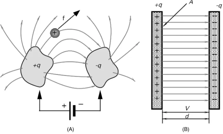
3.1 Electric Charges, Fields, and Potentials . . . 38
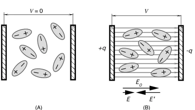
3.2 Capacitance . . . 44
3.2.1 Capacitor . . . 45
3.2.2 Dielectric Constant . . . 46
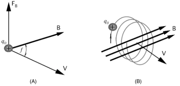
3.3 Magnetism . . . 50
3.3.1 Faraday’s Law . . . 52
3.3.2 Solenoid . . . 54
3.3.3 Toroid . . . 55
3.3.4 Permanent Magnets . . . 55
3.4 Induction . . . 56
3.5 Resistance . . . 59
3.5.1 Specific Resistivity . . . 60
3.5.2 Temperature Sensitivity . . . 62
3.5.3 Strain Sensitivity . . . 64
3.5.4 Moisture Sensitivity . . . 65
3.6 Piezoelectric Effect . . . 66
3.6.1 Piezoelectric Films . . . 72
3.7 Pyroelectric Effect . . . 76
3.8 Hall Effect . . . 82
3.9 Seebeck and Peltier Effects . . . 86
3.10 Sound Waves . . . 92
3.11 Temperature and Thermal Properties of Materials . . . 94
3.11.1 Temperature Scales . . . 95
3.11.2 Thermal Expansion . . . 96
3.11.3 Heat Capacity . . . 98
3.12 Heat Transfer . . . 99
3.12.1 Thermal Conduction . . . 99
3.12.2 Thermal Convection . . . 102
3.12.3 Thermal Radiation . . . 103
3.12.3.1 Emissivity . . . 106
3.12.3.2 Cavity Effect . . . 109
3.13 Light . . . 111
3.14 Dynamic Models of Sensor Elements . . . 113
3.14.1 Mechanical Elements . . . 115
3.14.2 Thermal Elements . . . 117
3.14.3 Electrical Elements . . . 118
3.14.4 Analogies . . . 119
References . . . 119
4 Optical Components of Sensors . . . 123
4.1 Radiometry. . . 125
4.2 Photometry . . . 129
4.3 Windows . . . 132
Contents XI
4.5 Lenses . . . 136
4.6 Fresnel Lenses . . . 137
4.7 Fiber Optics and Waveguides . . . 140
4.8 Concentrators . . . 144
4.9 Coatings for Thermal Absorption . . . 145
4.10 Electro-optic and Acousto-optic Modulators . . . 146
4.11 Interferometric Fiber-optic Modulation . . . 148
References . . . 149
5 Interface Electronic Circuits. . . 151
5.1 Input Characteristics of Interface Circuits . . . 151
5.2 Amplifiers . . . 156
5.2.1 Operational Amplifiers . . . 156
5.2.2 Voltage Follower . . . 158
5.2.3 Instrumentation Amplifier . . . 159
5.2.4 Charge Amplifiers . . . 161
5.3 Excitation Circuits . . . 164
5.3.1 Current Generators . . . 165
5.3.2 Voltage References . . . 169
5.3.3 Oscillators . . . 171
5.3.4 Drivers . . . 174
5.4 Analog-to-Digital Converters . . . 175
5.4.1 Basic Concepts . . . 175
5.4.2 V/F Converters . . . 176
5.4.3 Dual-Slope Converter . . . 181
5.4.4 Successive-Approximation Converter . . . 183
5.4.5 Resolution Extension . . . 185
5.5 Direct Digitization and Processing . . . 186
5.6 Ratiometric Circuits . . . 190
5.7 Bridge Circuits . . . 192
5.7.1 Disbalanced Bridge . . . 193
5.7.2 Null-Balanced Bridge . . . 194
5.7.3 Temperature Compensation of Resistive Bridge . . . 195
5.7.4 Bridge Amplifiers . . . 200
5.8 Data Transmission . . . 201
5.8.1 Two-Wire Transmission . . . 202
5.8.2 Four-Wire Sensing . . . 203
5.8.3 Six-Wire Sensing . . . 204
5.9 Noise in Sensors and Circuits . . . 204
5.9.1 Inherent Noise . . . 205
5.9.2 Transmitted Noise . . . 207
5.9.3 Electric Shielding . . . 212
5.9.4 Bypass Capacitors . . . 214
5.9.5 Magnetic Shielding . . . 215
5.9.7 Ground Planes . . . 218
5.9.8 Ground Loops and Ground Isolation . . . 219
5.9.9 Seebeck Noise . . . 221
5.10 Batteries for Low Power Sensors . . . 222
5.10.1 Primary Cells . . . 223
5.10.2 Secondary Cells . . . 224
References . . . 225
6 Occupancy and Motion Detectors. . . 227
6.1 Ultrasonic Sensors . . . 228
6.2 Microwave Motion Detectors . . . 228
6.3 Capacitive Occupancy Detectors . . . 233
6.4 Triboelectric Detectors . . . 237
6.5 Optoelectronic Motion Detectors . . . 238
6.5.1 Sensor Structures . . . 240
6.5.1.1 Multiple Sensors . . . 241
6.5.1.2 Complex Sensor Shape . . . 241
6.5.1.3 Image Distortion . . . 241
6.5.1.4 Facet Focusing Element . . . 242
6.5.2 Visible and Near-Infrared Light Motion Detectors . . . 243
6.5.3 Far-Infrared Motion Detectors . . . 244
6.5.3.1 PIR Motion Detectors . . . 245
6.5.3.2 PIR Sensor Efficiency Analysis . . . 247
References . . . 251
7 Position, Displacement, and Level . . . 253
7.1 Potentiometric Sensors . . . 254
7.2 Gravitational Sensors . . . 256
7.3 Capacitive Sensors . . . 258
7.4 Inductive and Magnetic Sensors . . . 262
7.4.1 LVDT and RVDT . . . 262
7.4.2 Eddy Current Sensors . . . 264
7.4.3 Transverse Inductive Sensor . . . 266
7.4.4 Hall Effect Sensors . . . 267
7.4.5 Magnetoresistive Sensors . . . 271
7.4.6 Magnetostrictive Detector . . . 274
7.5 Optical Sensors . . . 275
7.5.1 Optical Bridge . . . 275
7.5.2 Proximity Detector with Polarized Light . . . 276
7.5.3 Fiber-Optic Sensors . . . 278
7.5.4 Fabry–Perot Sensors . . . 278
7.5.5 Grating Sensors . . . 281
7.5.6 Linear Optical Sensors (PSD) . . . 283
7.6 Ultrasonic Sensors . . . 286
Contents XIII
7.7.1 Micropower Impulse Radar . . . 289
7.7.2 Ground-Penetrating Radar . . . 291
7.8 Thickness and Level Sensors . . . 293
7.8.1 Ablation Sensors . . . 293
7.8.2 Thin-Film Sensors . . . 296
7.8.3 Liquid-Level Sensors . . . 296
References . . . 298
8 Velocity and Acceleration. . . 301
8.1 Accelerometer Characteristics . . . 303
8.2 Capacitive Accelerometers . . . 305
8.3 Piezoresistive Accelerometers . . . 307
8.4 Piezoelectric Accelerometers . . . 309
8.5 Thermal Accelerometers . . . 309
8.5.1 Heated-Plate Accelerometer . . . 309
8.5.2 Heated-Gas Accelerometer . . . 310
8.6 Gyroscopes . . . 313
8.6.1 Rotor Gyroscope . . . 313
8.6.2 Monolithic Silicon Gyroscopes . . . 314
8.6.3 Optical Gyroscopes . . . 317
8.7 Piezoelectric Cables . . . 319
References . . . 321
9 Force, Strain, and Tactile Sensors. . . 323
9.1 Strain Gauges . . . 325
9.2 Tactile Sensors . . . 327
9.3 Piezoelectric Force Sensors . . . 334
References . . . 336
10 Pressure Sensors. . . 339
10.1 Concepts of Pressure . . . 339
10.2 Units of Pressure . . . 340
10.3 Mercury Pressure Sensor . . . 341
10.4 Bellows, Membranes, and Thin Plates . . . 342
10.5 Piezoresistive Sensors . . . 344
10.6 Capacitive Sensors . . . 349
10.7 VRP Sensors . . . 350
10.8 Optoelectronic Sensors . . . 352
10.9 Vacuum Sensors . . . 354
10.9.1 Pirani Gauge . . . 354
10.9.2 Ionization Gauges . . . 356
10.9.3 Gas Drag Gauge . . . 356
11 Flow Sensors . . . 359
11.1 Basics of Flow Dynamics . . . 359
11.2 Pressure Gradient Technique . . . 361
11.3 Thermal Transport Sensors . . . 363
11.4 Ultrasonic Sensors . . . 367
11.5 Electromagnetic Sensors . . . 370
11.6 Microflow Sensors . . . 372
11.7 Breeze Sensor . . . 374
11.8 Coriolis Mass Flow Sensors . . . 376
11.9 Drag Force Flow Sensors . . . 377
References . . . 378
12 Acoustic Sensors . . . 381
12.1 Resistive Microphones . . . 382
12.2 Condenser Microphones . . . 382
12.3 Fiber-Optic Microphone . . . 383
12.4 Piezoelectric Microphones . . . 385
12.5 Electret Microphones . . . 386
12.6 Solid-State Acoustic Detectors . . . 388
References . . . 391
13 Humidity and Moisture Sensors . . . 393
13.1 Concept of Humidity . . . 393
13.2 Capacitive Sensors . . . 396
13.3 Electrical Conductivity Sensors . . . 399
13.4 Thermal Conductivity Sensor . . . 401
13.5 Optical Hygrometer . . . 402
13.6 Oscillating Hygrometer . . . 403
References . . . 404
14 Light Detectors . . . 407
14.1 Introduction . . . 407
14.2 Photodiodes . . . 411
14.3 Phototransistor . . . 418
14.4 Photoresistors . . . 420
14.5 Cooled Detectors . . . 423
14.6 Thermal Detectors . . . 425
14.6.1 Golay Cells . . . 426
14.6.2 Thermopile Sensors . . . 427
14.6.3 Pyroelectric Sensors . . . 430
14.6.4 Bolometers . . . 434
14.6.5 Active Far-Infrared Sensors . . . 437
14.7 Gas Flame Detectors . . . 439
Contents XV
15 Radiation Detectors . . . 443
15.1 Scintillating Detectors. . . 444
15.2 Ionization Detectors . . . 447
15.2.1 Ionization Chambers . . . 447
15.2.2 Proportional Chambers . . . 449
15.2.3 Geiger–Müller Counters . . . 450
15.2.4 Semiconductor Detectors . . . 451
References . . . 455
16 Temperature Sensors . . . 457
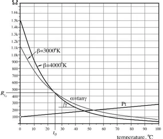
16.1 Thermoresistive Sensors . . . 461
16.1.1 Resistance Temperature Detectors . . . 461
16.1.2 Silicon Resistive Sensors . . . 464
16.1.3 Thermistors . . . 465
16.1.3.1 NTC Thermistors . . . 465
16.1.3.2 Self-Heating Effect in NTC Thermistors . . . 474
16.1.3.3 PTC Thermistors . . . 477
16.2 Thermoelectric Contact Sensors . . . 481
16.2.1 Thermoelectric Law . . . 482
16.2.2 Thermocouple Circuits . . . 484
16.2.3 Thermocouple Assemblies . . . 486
16.3 Semiconductor P-N Junction Sensors . . . 488
16.4 Optical Temperature Sensors . . . 491
16.4.1 Fluoroptic Sensors . . . 492
16.4.2 Interferometric Sensors . . . 494
16.4.3 Thermochromic Solution Sensor . . . 494
16.5 Acoustic Temperature Sensor . . . 495
16.6 Piezoelectric Temperature Sensors . . . 496
References . . . 497
17 Chemical Sensors . . . 499
17.1 Chemical Sensor Characteristics . . . 500
17.2 Specific Difficulties . . . 500
17.3 Classification of Chemical-Sensing Mechanisms . . . 501
17.4 Direct Sensors . . . 503
17.4.1 Metal-Oxide Chemical Sensors . . . 503
17.4.2 ChemFET . . . 504
17.4.3 Electrochemical Sensors . . . 505
17.4.4 Potentiometric Sensors . . . 506
17.4.5 Conductometric Sensors . . . 507
17.4.6 Amperometric Sensors . . . 508
17.4.7 Enhanced Catalytic Gas Sensors . . . 510
17.4.8 Elastomer Chemiresistors . . . 512
17.5 Complex Sensors . . . 512
17.5.2 Pellister Catalytic Sensors . . . 514
17.5.3 Optical Chemical Sensors . . . 514
17.5.4 Mass Detector . . . 516
17.5.5 Biochemical Sensors . . . 519
17.5.6 Enzyme Sensors . . . 520
17.6 Chemical Sensors Versus Instruments . . . 520
17.6.1 Chemometrics . . . 523
17.6.2 Multisensor Arrays . . . 524
17.6.3 Electronic Noses (Olfactory Sensors) . . . 524
17.6.4 Neural Network Signal (Signature) Processing for Electronic Noses . . . 527
17.6.5 “Smart” Chemical Sensors . . . 530
References . . . 530
18 Sensor Materials and Technologies. . . 533
18.1 Materials . . . 533
18.1.1 Silicon as a Sensing Material . . . 533
18.1.2 Plastics . . . 536
18.1.3 Metals . . . 540
18.1.4 Ceramics . . . 542
18.1.5 Glasses . . . 543
18.2 Surface Processing . . . 543
18.2.1 Deposition of Thin and Thick Films . . . 543
18.2.2 Spin-Casting . . . 544
18.2.3 Vacuum Deposition . . . 544
18.2.4 Sputtering . . . 545
18.2.5 Chemical Vapor Deposition . . . 546
18.3 Nano-Technology . . . 547
18.3.1 Photolithography . . . 548
18.3.2 Silicon Micromachining . . . 549
18.3.2.1 Basic Techniques . . . 549
18.3.2.2 Wafer bonding . . . 554
References . . . 555
Appendix . . . 557
Table A.1 Chemical Symbols for the Elements . . . 557
Table A.2 SI Multiples . . . 558
Table A.3 Derivative SI Units . . . 558
Table A.4 SI Conversion Multiples . . . 559
Table A.5 Dielectric Constants of Some Materials at Room Temperature . . . 564
Table A.6 Properties of Magnetic Materials . . . 564
Table A.7 Resistivities and Temperature Coefficients of Resistivity of Some Materials at Room Temperature . . . . 565
Contents XVII
Table A.9 Physical Properties of Pyroelectric Materials . . . 566
Table A.10 Characteristics of Thermocouple Types . . . 566
Table A.11 Thermoelectric Coefficients and Volume Resistivities of Selected Elements . . . 567
Table A.11a Thermocouples for Very Low and Very High Temperatures . . . 567
Table A.12 Densities of Some Materials . . . 568
Table A.13 Mechanical Properties of Some Solid Materials . . . 568
Table A.14 Mechanical Properties of Some Crystalline Materials . . . 569
Table A.15 Speed of Sound Waves . . . 569
Table A.16 Coefficient of Linear Thermal Expansion of Some Materials . . . 569
Table A.17 Specific Heat and Thermal Conductivity of Some Materials . . . 570
Table A.18 Typical Emissivities of Different Materials . . . 571
Table A.19 Refractive Indices of Some Materials . . . 572
Table A.20 Characteristics of C–Zn and Alkaline Cells . . . 573
Table A.21 Lithium–Manganese Dioxide Primary Cells . . . 573
Table A.22 Typical Characteristics of “AA”-Size Secondary Cells . . . 573
Table A.23 Miniature Secondary Cells and Batteries . . . 574
Table A.24 Electronic Ceramics . . . 576
Table A.25 Properties of Glasses . . . 577
1
Data Acquisition
“It’s as large as life, and twice as natural”
—Lewis Carroll, “Through the Looking Glass”
1.1 Sensors, Signals, and Systems
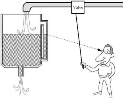
Fig. 1.1.Level-control system. A sight tube and operator’s eye form a sensor (a device which converts information into electrical signal).
information is also transmitted and processed in electrical form—however, through the transport of electrons. Sensors that are used in artificial systems must speak the same language as the devices with which they are interfaced. This language is electri-cal in its nature and a man-made sensor should be capable of responding with signals where information is carried by displacement of electrons, rather than ions.1Thus,
it should be possible to connect a sensor to an electronic system through electrical wires, rather than through an electrochemical solution or a nerve fiber. Hence, in this book, we use a somewhat narrower definition of sensors, which may be phrased as
A sensor is a device that receives a stimulus and responds with an electrical signal.
The termstimulusis used throughout this book and needs to be clearly understood. The stimulus is the quantity, property, or condition that is sensed and converted into electrical signal. Some texts (for instance, Ref. [2]) use a different term,measurand, which has the same meaning, however with the stress on quantitative characteristic of sensing.
The purpose of a sensor is to respond to some kind of an input physical property (stimulus) and to convert it into an electrical signal which is compatible with electronic circuits. We may say that a sensor is a translator of a generally nonelectrical value into an electrical value. When we say “electrical,” we mean a signal which can be channeled, amplified, and modified by electronic devices. The sensor’s output signal may be in the form of voltage, current, or charge. These may be further described in terms of amplitude, frequency, phase, or digital code. This set of characteristics is called theoutput signal format. Therefore, a sensor has input properties (of any kind) and electrical output properties.
1There is a very exciting field of the optical computing and communications where
1.1 Sensors, Signals, and Systems 3
Fig. 1.2.A sensor may incorporate several transducers.e1, e2,and so on are various types of
energy. Note that the last part is a direct sensor.
Any sensor is an energy converter. No matter what you try to measure, you al-ways deal with energy transfer from the object of measurement to the sensor. The process of sensing is a particular case of information transfer, and any transmission of information requires transmission of energy. Of course, one should not be confused by an obvious fact that transmission of energy can flow both ways—it may be with a positive sign as well as with a negative sign; that is, energy can flow either from an object to the sensor or from the sensor to the object. A special case is when the energy is zero, and it also carries information about existence of that particular case. For example, a thermopile infrared radiation sensor will produce a positive voltage when the object is warmer than the sensor (infrared flux is flowing to the sensor) or the voltage is negative when the object is cooler than the sensor (infrared flux flows from the sensor to the object). When both the sensor and the object are at the same temperature, the flux is zero and the output voltage is zero. This carries a message that the temperatures are the same.
The termsensorshould be distinguished fromtransducer. The latter is a converter of one type of energy into another, whereas the former converts any type of energy into electrical. An example of a transducer is a loudspeaker which converts an electrical signal into a variable magnetic field and, subsequently, into acoustic waves.2This is
nothing to do with perception or sensing. Transducers may be used asactuatorsin various systems. An actuator may be described as opposite to a sensor—it converts electrical signal into generally nonelectrical energy. For example, an electric motor is an actuator—it converts electric energy into mechanical action.
Transducers may be parts of complex sensors (Fig. 1.2). For example, a chemical sensor may have a part which converts the energy of a chemical reaction into heat (transducer) and another part, a thermopile, which converts heat into an electrical sig-nal. The combination of the two makes a chemical sensor—a device which produces anelectricalsignal in response to a chemical reaction. Note that in the above example, a chemical sensor is a complex sensor; it is comprised of a transducer and another sensor (heat). This suggests that many sensors incorporate at least onedirect-type sensor and a number of transducers. The direct sensors are those that employ such physical effects that make adirect energy conversion into electrical signal genera-tion or modificagenera-tion. Examples of such physical effects are photoeffect and Seebeck effect. These will be described in Chapter 3.
2It is interesting to note that a loudspeaker, when connected to an input of an amplifier, may
In summary, there are two types of sensors:directandcomplex. A direct sensor converts a stimulus into an electrical signal or modifies an electrical signal by using an appropriate physical effect, whereas a complex sensor in addition needs one or more transducers of energy before a direct sensor can be employed to generate an electrical output.
A sensor does not function by itself; it is always a part of a larger system that may incorporate many other detectors, signal conditioners, signal processors, memory devices, data recorders, and actuators. The sensor’s place in a device is either intrinsic or extrinsic. It may be positioned at the input of a device to perceive the outside effects and to signal the system about variations in the outside stimuli. Also, it may be an internal part of a device that monitors the devices’ own state to cause the appropriate performance. A sensor is always a part of some kind of a data acquisition system. Often, such a system may be a part of a larger control system that includes various feedback mechanisms.
To illustrate the place of sensors in a larger system, Fig. 1.3 shows a block diagram of a data acquisition and control device. An object can be anything: a car, space ship, animal or human, liquid, or gas. Any material object may become a subject of some kind of a measurement. Data are collected from an object by a number of sensors. Some of them (2, 3, and 4) are positioned directly on or inside the object. Sensor 1 perceives the object without a physical contact and, therefore, is called anoncontact sensor. Examples of such a sensor is a radiation detector and a TV camera. Even if
Fig. 1.3.Positions of sensors in a data acquisition system. Sensor 1 is noncontact, sensors 2
1.1 Sensors, Signals, and Systems 5
we say “noncontact”, we remember that energy transfer always occurs between any sensor and an object.
Sensor 5 serves a different purpose. It monitors internal conditions of a data acquisition system itself. Some sensors (1 and 3) cannot be directly connected to standard electronic circuits because of inappropriate output signal formats. They re-quire the use of interface devices (signal conditioners). Sensors 1, 2, 3, and 5 are passive. They generate electric signals without energy consumption from the elec-tronic circuits. Sensor 4 is active. It requires an operating signal, which is provided by an excitation circuit. This signal is modified by the sensor in accordance with the converted information. An example of an active sensor is a thermistor, which is a temperature-sensitive resistor. It may operate with a constant-current source, which is an excitation circuit. Depending on the complexity of the system, the total number of sensors may vary from as little as one (a home thermostat) to many thousands (a space shuttle).
Electrical signals from the sensors are fed into a multiplexer (MUX), which is a switch or a gate. Its function is to connect sensors one at a time to an analog-to-digital (A/D) converter if a sensor produces an analog signal, or directly to a computer if a sensor produces signals in a digital format. The computer controls a multiplexer and an A/D converter for the appropriate timing. Also, it may send control signals to the actuator, which acts on the object. Examples of actuators are an electric motor, a solenoid, a relay, and a pneumatic valve. The system contains some peripheral devices (for instance, a data recorder, a display, an alarm, etc.) and a number of components, which are not shown in the block diagram. These may be filters, sample-and-hold circuits, amplifiers, and so forth.
To illustrate how such a system works, let us consider a simple car-door monitoring arrangement. Every door in a car is supplied with a sensor which detects the door position (open or closed). In most cars, the sensor is a simple electric switch. Signals from all door sensors go to the car’s internal microprocessor (no need for an A/D converter as all door signals are in a digital format: ones or zeros). The microprocessor identifies which door is open and sends an indicating signal to the peripheral devices (a dashboard display and an audible alarm). A car driver (the actuator) gets the message and acts on the object (closes the door).
An example of a more complex device is an anesthetic vapor delivery system. It is intended for controlling the level of anesthetic drugs delivered to a patient by means of inhalation during surgical procedures. The system employs several active and passive sensors. The vapor concentration of anesthetic agents (such as halothane, isoflurane, or enflurane) is selectively monitored by an active piezoelectric sensor, installed into a ventilation tube. Molecules of anesthetic vapors add mass to the oscillating crystal in the sensor and change its natural frequency, which is a measure of vapor concentration. Several other sensors monitor the concentration of CO2, to
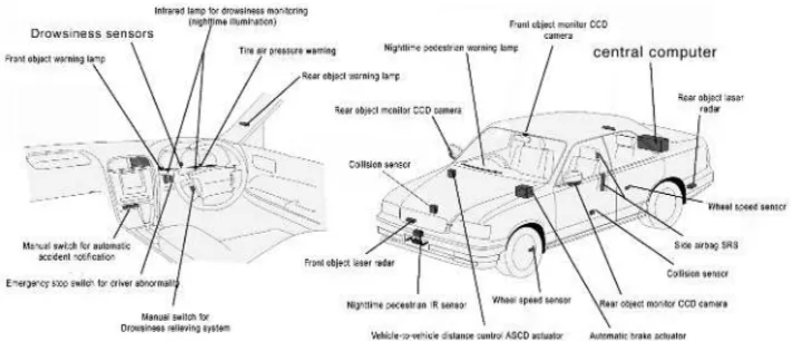
Fig. 1.4.Multiple sensors, actuators, and warning signals are parts of the Advanced Safety Vehicle. (Courtesy of Nissan Motor Company.)
Another example of a complex combination of various sensors, actuators, and indicating signals is shown in Fig. 1.4. It is an Advanced Safety Vehicle (ASV) that is being developed by Nissan. The system is aimed at increasing safety of a car. Among many others, it includes a drowsiness warning system and drowsiness relieving sys-tem. This may include the eyeball movement sensor and the driver head inclination detector. The microwave, ultrasonic, and infrared range measuring sensors are incor-porated into the emergency braking advanced advisory system to illuminate the break lamps even before the driver brakes hard in an emergency, thus advising the driver of a following vehicle to take evasive action. The obstacle warning system includes both the radar and infrared (IR) detectors. The adaptive cruise control system works if the driver approaches too closely to a preceding vehicle: The speed is automatically reduced to maintain a suitable safety distance. The pedestrian monitoring system de-tects and alerts the driver to the presence of pedestrians at night as well as in vehicle blind spots. The lane control system helps in the event that the system detects and de-termines that incipient lane deviation is not the driver’s intention. It issues a warning and automatically steers the vehicle, if necessary, to prevent it from leaving its lane. In the following chapters, we concentrate on methods of sensing, physical princi-ples of sensors operations, practical designs, and interface electronic circuits. Other essential parts of the control and monitoring systems, such as actuators, displays, data recorders, data transmitters, and others, are beyond the scope of this book and mentioned only briefly.
Generally, the sensor’s input signals (stimuli) may have almost any conceivable physical or chemical nature (e.g., light flux, temperature, pressure, vibration, dis-placement, position, velocity, ion concentration, . . .). The sensor’s design may be
1.2 Sensor Classification 7
oscillometric method with an inflatable cuff. Some sensors are specifically designed to be very selective in a particular range of input stimulus and be quite immune to signals outside of the desirable limits. For instance, a motion detector for a security system should be sensitive to movement of humans and not responsive to movement of smaller animals, like dogs and cats.
1.2 Sensor Classification
Sensor classification schemes range from very simple to the complex. Depending on the classification purpose, different classification criteria may be selected. Here, we offer several practical ways to look at the sensors.
All sensors may be of two kinds: passiveand active. A passive sensor does not need any additional energy source and directly generates an electric signal in response to an external stimulus; that is, the input stimulus energy is converted by the sensor into the output signal. The examples are a thermocouple, a photodiode, and a piezoelectric sensor. Most of passive sensors are direct sensors as we defined them earlier. The active sensors require external power for their operation, which is called an excitation signal. That signal is modified by the sensor to produce the output signal. The active sensors sometimes are called parametric because their own properties change in response to an external effect and these properties can be subsequently converted into electric signals. It can be stated that a sensor’s parameter modulates the excitation signal and that modulation carries information of the measured value. For example, a thermistor is a temperature-sensitive resistor. It does not generate any electric signal, but by passing an electric current through it (excitation signal), its resistance can be measured by detecting variations in current and/or voltage across the thermistor. These variations (presented in ohms) directly relate to ttemperature through a known function. Another example of an active sensor is a resistive strain gauge in which electrical resistance relates to a strain. To measure the resistance of a sensor, electric current must be applied to it from an external power source.
Depending on the selected reference, sensors can be classified intoabsoluteand relative. Anabsolutesensor detects a stimulus in reference to an absolute physical scale that is independent on the measurement conditions, whereas arelativesensor produces a signal that relates to some special case. An example of an absolute sensor is a thermistor: a temperature-sensitive resistor. Its electrical resistance directly relates to the absolute temperature scale of Kelvin.Another very popular temperature sensor—a thermocouple—is a relative sensor. It produces an electric voltage that is function of a temperature gradient across the thermocouple wires. Thus, a thermocouple output signal cannot be related to any particular temperature without referencing to a known baseline. Another example of the absolute and relative sensors is a pressure sensor. An absolute-pressure sensor produces signal in reference to vacuum—an absolute zero on a pressure scale. A relative-pressure sensor produces signal with respect to a selected baseline that is not zero pressure (e.g., to the atmospheric pressure).
sensitive to, what conversion mechanism is employed, what material it is fabricated from, and what its field of application is. Tables 1.1–1.6, adapted from Ref. [3], represent such a classification scheme, which is pretty much broad and representative. If we take for the illustration a surface acoustic-wave oscillator accelerometer, the table entries might be as follows:
Stimulus: Acceleration
Specifications: Sensitivity in frequency shift per gram of acceleration, short- and long-term stability in Hz per unit time, etc. Detection means: Mechanical
Conversion phenomenon: Elastoelectric Material: Inorganic insulator
Field: Automotive, marine, space, and scientific measurement
Table 1.1.Specifications
Sensitivity Stimulus range (span) Stability (short and long term) Resolution
Accuracy Selectivity
Speed of response Environmental conditions Overload characteristics Linearity
Hysteresis Dead band
Operating life Output format Cost, size, weight Other
Table 1.2.Sensor Material
Inorganic Organic
Conductor Insulator
Semiconductor Liquid, gas, or plasma Biological substance Other
Table 1.3.Detection Means Used in Sensors
Biological Chemical
Electric, magnetic, or electromagnetic wave Heat, temperature
Mechanical displacement or wave Radioactivity, radiation
1.3 Units of Measurements 9
Table 1.4.Conversion Phenomena
Physical Chemical
Thermoelectric Chemical transformation Photoelectric Physical transformation Photomagnetic Electrochemical process Magnetoelectric Spectroscopy
Electromagnetic Other Thermoelastic Biological
Electroelastic Biochemical transformation Thermomagnetic Physical transformation Thermooptic Effect on test organism Photoelastic Spectroscopy
Other Other
Table 1.5.Field of Applications
Agriculture Automotive
Civil engineering, construction Domestic, appliances
Distribution, commerce, finance Environment, meteorology, security Energy, power Information, telecommunication
Health, medicine Marine
Manufacturing Recreation, toys
Military Space
Scientific measurement Other Transportation (excluding automotive)
1.3 Units of Measurements
In this book, we use base units which have been established in The 14th General Conference on Weights and Measures (1971). The base measurement system is known as SI which stands for French“Le Systéme International d’Unités”(Table 1.7) [4]. All other physical quantities are derivatives of these base units. Some of them are listed in Table A.3.
Often, it is not convenient to use base or derivative units directly; in practice, quantities may be either too large or too small. For convenience in the engineering work, multiples and submultiples of the units are generally employed. They can be obtained by multiplying a unit by a factor from Table A.2. When pronounced, in all cases the first syllable is accented. For example, 1 ampere (A) may be multiplied by factor of 10−3to obtain a smaller unit: 1 milliampere (mA), which is one-thousandth
of an ampere.
Table 1.6.Stimulus
Acoustic Mechanical
Wave amplitude, phase, polarization Position (linear, angular)
Spectrum Acceleration
Wave velocity Force
Other Stress, pressure
Biological Strain
Biomass (types, concentration, states) Mass, density
Other Moment, torque
Chemical Speed of flow,rate of mass transport
Components (identities, concentration, states) Shape, roughness, orientation
Other Stiffness, compliance
Electric Viscosity
Charge, current Crystallinity, structural integrity
Potential, voltage Other
Electric field (amplitude, phase, Radiation
polarization, spectrum) Type
Conductivity Energy
Permitivity Intensity
Other Other
Magnetic Thermal
Magnetic field (amplitude, phase, Temperature
polarization, spectrum) Flux
Magnetic flux Specific heat
Permeability Thermal conductivity
Other Other
Optical
Wave amplitude, phase, polarization, spectrum Wave velocity
Refractive index Emissivity
reflectivity, absorption Other
still is not in common use. However, with the end of communism and the increase of world integration, international cooperation gains strong momentum. Hence, it is unavoidable that the United States will convert to SI3in the future, although maybe
not in our lifetime. Still, in this book, we will generally use SI; however, for the convenience of the reader, the U.S. customary system units will be used in places where U.S. manufacturers employ them for sensor specifications. For the conversion to SI from other systems,4the reader may use Tables A.4. To make a conversion, a
3SI is often called the modernized metric system.
4Nomenclature, abbreviations, and spelling in the conversion tables are in accordance with
References 11
Table 1.7.SI Basic Units
Quantity Name Symbol Defined by (Year Established) Length Meter m The length of the path traveled by light
in vacuum in 1/299,792,458 of a second. (1983)
Mass Kilogram kg After a platinum–iridium prototype (1889) Time Second s The duration of 9,192,631,770 periods of
the radiation corresponding to the transition between the two hyperfine levels of the ground state of the cesium-133 atom (1967)
Electric current Ampere A Force equal to 2×10⁻⁷Nm of length exerted on two parallel conductors in vacuum when they carry the current (1946) Thermodynamic Kelvin K The fraction 1/273.16 of the thermodynamic
temperature temperature of the triple point of water length(1967)
Amount of substance Mole mol The amount of substance which contains as many elementary entities as there are atoms in 0.012 kg of carbon 12 (1971) Luminous intensity Candela cd Intensity in the perpendicular direction of a
surface of 1/600,000 m2of a blackbody at temperature of freezing Pt under pressure of 101,325 Nm2(1967)
Plane angle Radian rad (Supplemental unit) Solid angle Steradian sr (Supplemental unit)
non-SI value should be multiplied by a number given in the table. For instance, to convert an acceleration of 55 ft/s2to SI, it must to be multiplied by 0.3048:
55ft/s2×0.3048=16.764 m/s2
Similarly, to convert an electric charge of 1.7 faraday, it must be multiplied by 9.65×10¹⁹:
1.7 faraday×9.65×1019=1.64×10²⁰C
The reader should consider the correct terminology of the physical and technical terms. For example, in the United States and many other countries, the electric po-tential difference is called “voltage,” whereas in other countries, “electric tension” or simply “tension” is in common use. In this book, we use terminology that is traditional in the United States.
References
2. Norton, H. N. Handbook of Transducers. Prentice-Hall, Englewood Cliffs, NJ, 1989.
3. White, R. W. A sensor classification scheme. In:Microsensors. IEEE Press, New York, 1991, pp. 3–5.
2
Sensor Characteristics
“O, what men dare do! What men may do! What men daily do, not knowing what they do.”
—Shakespeare, “Much Ado About Nothing”
From the input to the output, a sensor may have several conversion steps before it produces an electrical signal. For instance, pressure inflicted on the fiber-optic sensor first results in strain in the fiber, which, in turn, causes deflection in its refractive index, which, in turn, results in an overall change in optical transmission and modulation of photon density. Finally, photon flux is detected and converted into electric current. In this chapter, we discuss the overall sensor characteristics, regardless of its physical nature or steps required to make a conversion. We regard a sensor as a “black box” where we are concerned only with relationships between its output signal and input stimulus.
2.1 Transfer Function
Anidealortheoreticaloutput–stimulus relationship exists for every sensor. If the sen-sor is ideally designed and fabricated with ideal materials by ideal workers using ideal tools, the output of such a sensor would always represent thetruevalue of the stimulus. The ideal function may be stated in the form of a table of values, a graph, or a mathe-matical equation. An ideal (theoretical) output–stimulus relationship is characterized by the so-calledtransfer function. This function establishes dependence between the electrical signalS produced by the sensor and the stimuluss:S=f (s). That
func-tion may be a simple linear connecfunc-tion or a nonlinear dependence, (e.g., logarithmic, exponential, or power function). In many cases, the relationship is unidimensional (i.e., the output versus one input stimulus). A unidimensional linear relationship is represented by the equation
whereais the intercept (i.e., the output signal at zero input signal) andbis the slope,
which is sometimes calledsensitivity.S is one of the characteristics of the output
electric signal used by the data acquisition devices as the sensor’s output. It may be amplitude, frequency, or phase, depending on the sensor properties.
Logarithmic function:
S=a+blns. (2.2)
Exponential function:
S=aeks. (2.3)
Power function:
S=a0+a1sk, (2.4)
wherekis a constant number.
A sensor may have such a transfer function that none of the above approximations fits sufficiently well. In that case, a higher-order polynomial approximation is often employed.
For a nonlinear transfer function, the sensitivitybis not a fixed number as for the
linear relationship [Eq. (2.1)]. At any particular input value,s0, it can be defined as
b=dS(s0)
ds . (2.5)
In many cases, a nonlinear sensor may be considered linear over a limited range. Over the extended range, a nonlinear transfer function may be modeled by several straight lines. This is called a piecewise approximation. To determine whether a function can be represented by a linear model, the incremental variables are introduced for the input while observing the output. A difference between the actual response and a liner model is compared with the specified accuracy limits (see 2.4).
A transfer function may have more than one dimension when the sensor’s output is influenced by more than one input stimuli. An example is the transfer function of a thermal radiation (infrared) sensor. The function1connects two temperatures (Tb, the
absolute temperature of an object of measurement, andTs, the absolute temperature of the sensor’s surface) and the output voltageV:
V =G(Tb4−Ts4), (2.6)
whereGis a constant. Clearly, the relationship between the object’s temperature and
the output voltage (transfer function) is not only nonlinear (the fourth-order parabola) but also depends on the sensor’s surface temperature. To determine the sensitivity of the sensor with respect to the object’s temperature, a partial derivative will be calculated as
b= ∂V ∂Tb=
4GTb3. (2.7)
The graphical representation of a two-dimensional transfer function of Eq. (2.6) is shown in Fig. 2.1. It can be seen that each value of the output voltage can be uniquely
2.2 Span (Full-Scale Input) 15
Fig. 2.1.Two-dimensional transfer function of a thermal radiation sensor.
determined from two input temperatures. It should be noted that a transfer func-tion represents the input-to-output relafunc-tionship. However, when a sensor is used for measuring or detecting a stimulus, an inversed function (output-to-input) needs to be employed. When a transfer function is linear, the inversed function is very easy to compute. When it is nonlinear the task is more complex, and in many cases, the analytical solution may not lend itself to reasonably simple data processing. In these cases, an approximation technique often is the solution.
2.2 Span (Full-Scale Input)
Table 2.1.Relationship Among Power, Force (Voltage, Current), and Decibels
Power
ratio 1.023 1.26 10.0 100 103 104 105 106 107 108 109 1010
Force
ratio 1.012 1.12 3.16 10.0 31.6 100 316 103 3162 104 3×10⁴ 105 Decibels 0.1 1.0 10.0 20.0 30.0 40.0 50.0 60.0 70.0 80.0 90.0 100.0
definition, decibels are equal to 10 times the log of the ratio of powers (Table 2.1):
1 dB=10 logP2
P1. (2.8)
In a similar manner, decibels are equal to 20 times the log of the force, current, or voltage:
1 dB=20 logS2
S1. (2.9)
2.3 Full-Scale Output
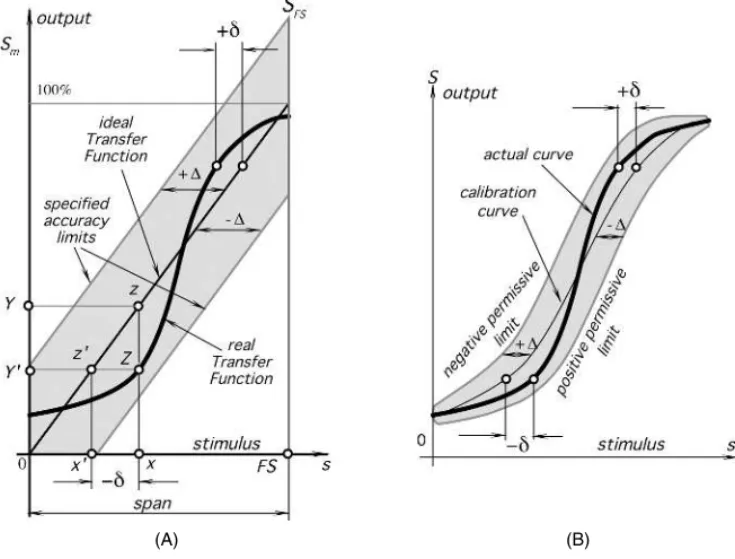
Full-scale output(FSO) is the algebraic difference between the electrical output sig-nals measured with maximum input stimulus and the lowest input stimulus applied. This must include all deviations from the ideal transfer function. For instance, the FSO output in Fig. 2.2A is represented bySFS.
(A) (B)
2.4 Accuracy 17
2.4 Accuracy
Avery important characteristic of a sensor isaccuracywhich really meansinaccuracy. Inaccuracy is measured as a highest deviation of a value represented by the sensor from the ideal or true value at its input. The true value is attributed to the object of measurement and accepted as having a specified uncertainty (see 2.20.)
The deviation can be described as a difference between the value which is com-puted from the output voltage and the actual input value. For example, a linear dis-placement sensor ideally should generate 1 mV per 1-mm disdis-placement; that is, its transfer function is linear with a slope (sensitivity) b=1 mV/mm. However,
in the experiment, a displacement of s=10 mm produced an output of S=10.5
mV. Converting this number into the displacement value by using the inversed transfer function (1/b=1 mm/mV), we would calculate that the displacement was sx=S/b=10.5 mm; that issx−s=0.5 mm more than the actual. This extra 0.5 mm is an erroneous deviation in the measurement, or error. Therefore, in a 10-mm range, the sensor’s absolute inaccuracy is 0.5 mm, or in the relative terms, inaccuracy is(0.5mm/10mm)×100%=5%. If we repeat this experiment over and over again
without any random error and every time we observe an error of 0.5 mm, we may say that the sensor has asystematicinaccuracy of 0.5 mm over a 10-mm span. Naturally, a random component is always present, so the systematic error may be represented as an average or mean value of multiple errors.
Figure 2.2A shows an ideal or theoretical transfer function. In the real world, any sensor performs with some kind of imperfection. A possiblerealtransfer function is represented by a thick line, which generally may be neither linear nor monotonic. A real function rarely coincides with the ideal. Because of material variations, work-manship, design errors, manufacturing tolerances, and other limitations, it is possible to have a large family of real transfer functions, even when sensors are tested under identical conditions. However, all runs of the real transfer functions must fall within the limits of a specified accuracy. These permissive limits differ from the ideal transfer function line by±. The real functions deviate from the ideal by±δ, whereδ≤.
For example, let us consider a stimulus having valuex. Ideally, we would expect this
value to correspond to pointzon the transfer function, resulting in the output value Y. Instead, the real function will respond at pointZ, producing output valueY′. This
output value corresponds to pointz′ on the ideal transfer function, which, in turn,
relates to a “would-be” input stimulusx′whose value is smaller thanx. Thus, in this
example, imperfection in the sensor’s transfer function leads to a measurement error of−δ.
The accuracy rating includes a combined effect of part-to-part variations, a hys-teresis, a dead band, calibration, and repeatability errors (see later subsections). The specified accuracy limits generally are used in the worst-case analysis to determine the worst possible performance of the system. Figure 2.2B shows that±may more
part-to-part variations between the sensors and are geared specifically to the cali-brated unit. Clearly, this method allows more accurate sensing; however, in some applications, it may be prohibitive because of a higher cost.
The inaccuracy rating may be represented in a number of forms: 1. Directly in terms of measured value()
2. In percent of input span (full scale) 3. In terms of output signal
For example, a piezoresistive pressure sensor has a 100-kPa input full scale and a 10
full-scale output. Its inaccuracy may be specified as±0.5%,±500 Pa, or±0.05.
In modern sensors, specification of accuracy often is replaced by a more compre-hensive value ofuncertainty(see Section 2.20) because uncertainty is comprised of all distorting effects both systematic and random and is not limited to the inaccuracy of a transfer function.
2.5 Calibration
If the sensor’s manufacturer’s tolerances and tolerances of the interface (signal condi-tioning) circuit are broader than the required system accuracy, a calibration is required. For example, we need to measure temperature with an accuracy±0.5◦C; however, an
available sensor is rated as having an accuracy of±1◦C. Does it mean that the sensor
can not be used? No, it can, but that particular sensor needs to be calibrated; that is, its individual transfer function needs to be found during calibration. Calibration means the determination of specific variables that describe the overall transfer func-tion. Overall means of the entire circuit, including the sensor, the interface circuit, and the A/D converter. The mathematical model of the transfer function should be known before calibration. If the model is linear [Eq. (2.1)], then the calibration should determine variablesaandb; if it is exponential [Eq. (2.3)], variablesaandkshould
be determined; and so on. Let us consider a simple linear transfer function. Because a minimum of two points are required to define a straight line, at least a two-point calibration is required. For example, if one uses a forward-biased semiconductor p-n junction for temperature measurement, with a high degree of accuracy its transfer function (temperature is the input and voltage is the output) can be considered linear:
v=a+bt. (2.10)
To determine constantsaandb, such a sensor should be subjected to two temperatures
(t1andt2) and two corresponding output voltages (v1andv2) will be registered. Then,
after substituting these values into Eq. (2.10), we arrive at
v1=a+bt1, (2.11)
v2=a+bt2,
and the constants are computed as
b=v1−v2
2.6 Calibration Error 19
To compute the temperature from the output voltage, a measured voltage is inserted into an inversed equation
t=v−a
b . (2.13)
In some fortunate cases, one of the constants may be specified with a sufficient accuracy so that no calibration of that particular constant may be needed. In the same p-n-junction temperature sensor, the slopebis usually a very consistent value for a
given lot and type of semiconductor. For example, a value ofb= −0.002268 V/◦C
was determined to be consistent for a selected type of the diode, then a single-point calibration is needed to find outaasa=v1+0.002268t1.
For nonlinear functions, more than two points may be required, depending on a mathematical model of the transfer function. Any transfer function may be modeled by a polynomial, and depending on required accuracy, the number of the calibration points should be selected. Because calibration may be a slow process, to reduce production cost in manufacturing, it is very important to minimize the number of calibration points.
Another way to calibrate a nonlinear transfer function is to use a piecewise ap-proximation. As was mentioned earlier, any section of a curvature, when sufficiently small, can be considered linear and modeled by Eq. (2.1). Then, a curvature will be described by a family of linear lines where each has its own constantsaandb.
Dur-ing the measurement, one should determine where on the curve a particular output voltageSis situated and select the appropriate set of constantsa andbto compute
the value of a corresponding stimulussfrom an equation identical to Eq. (2.13).
To calibrate sensors, it is essential to have and properly maintain precision and ac-curate physical standards of the appropriate stimuli. For example, to calibrate contact-temperature sensors, either a contact-temperature-controlled water bath or a “dry-well” cavity is required. To calibrate the infrared sensors, a blackbody cavity would be needed. To calibrate a hygrometer, a series of saturated salt solutions are required to sustain a constant relative humidity in a closed container, and so on. It should be clearly un-derstood that the sensing system accuracy is directly attached to the accuracy of the calibrator. An uncertainty of the calibrating standard must be included in the statement on the overall uncertainty, as explained in 2.20.
2.6 Calibration Error
Thecalibration erroris inaccuracy permitted by a manufacturer when a sensor is calibrated in the factory. This error is of a systematic nature, meaning that it is added to all possible real transfer functions. It shifts the accuracy of transduction for each stimulus point by a constant. This error is not necessarily uniform over the range and may change depending on the type of error in the calibration. For example, let us consider a two-point calibration of a real linear transfer function (thick line in Fig. 2.3). To determine the slope and the intercept of the function, two stimuli,s1
ands2, are applied to the sensor. The sensor responds with two corresponding output
Fig. 2.3.Calibration error.
the higher signal was measured with error−. This results in errors in the slope and
intercept calculation. A new intercept,a1, will differ from the real intercept,a, by δa=a1−a=
s2−s1, (2.14)
and the slope will be calculated with error:
δb= −
s2−s1, (2.15)
2.7 Hysteresis
Ahysteresis erroris a deviation of the sensor’s output at a specified point of the input signal when it is approached from the opposite directions (Fig. 2.4). For example, a displacement sensor when the object moves from left to right at a certain point produces a voltage which differs by 20 mV from that when the object moves from right to left. If the sensitivity of the sensor is 10 mV/mm, the hysteresis error in terms of displacement units is 2 mm. Typical causes for hysteresis are friction and structural changes in the materials.
2.8 Nonlinearity
Nonlinearityerror is specified for sensors whose transfer function may be approxi-mated by a straight line [Eq. (2.1)].Anonlinearity is a maximum deviation (L) of a real
2.8 Nonlinearity 21
Fig. 2.4.Transfer function with hysteresis.
means “nonlinearity.” When more than one calibration run is made, the worst linearity seen during any one calibration cycle should be stated. Usually, it is specified either in percent of span or in terms of measured value (e.g, in kPa or◦C). “Linearity,” when not accompanied by a statement explaining what sort of straight line it is referring to, is meaningless. There are several ways to specify a nonlinearity, depending how the line is superimposed on the transfer function. One way is to useterminalpoints (Fig. 2.5A); that is, to determine output values at the smallest and highest stimulus values and to draw a straight line through these two points (line 1). Here, near the terminal points, the nonlinearity error is the smallest and it is higher somewhere in between.
(A) (B)
Terminal Points
Fig. 2.5.Linear approximations of a nonlinear transfer function (A) and independent linearity
Another way to define the approximation line is to use a method ofleast squares (line 2 in Fig. 2.5A). This can be done in the following manner. Measure several(n)
output valuesS at input valuess over a substantially broad range, preferably over
an entire full scale. Use the following formulas for linear regression to determine interceptaand slopebof the best-fit straight line:
a=
S
s2−
s
sS n
s2−(
s)2 , b= n
sS−
s
S n
s2−(
s)2 , (2.16)
whereis the summation of
nnumbers.
In some applications, a higher accuracy may be desirable in a particular narrower section of the input range. For instance, a medical thermometer should have the best accuracy in a fever definition region which is between 37◦C and 38◦C. It may have a somewhat lower accuracy beyond these limits. Usually, such a sensor is calibrated in the region where the highest accuracy is desirable. Then, the approximation line may be drawn through the calibration pointc(line 3 in Fig. 2.5A). As a result, nonlinearity
has the smallest value near the calibration point and it increases toward the ends of the span. In this method, the line is often determined as tangent to the transfer function in pointc. If the actual transfer function is known, the slope of the line can be found
from Eq. (2.5).
Independent linearityis referred to as the so-called “best straight line” (Fig. 2.5B), which is a line midway between two parallel straight lines closest together and en-veloping all output values on a real transfer function.
Depending on the specification method, approximation lines may have different intercepts and slopes. Therefore, nonlinearity measures may differ quite substantially from one another.Auser should be aware that manufacturers often publish the smallest possible number to specify nonlinearity, without defining what method was used.
2.9 Saturation
Every sensor has its operating limits. Even if it is considered linear, at some levels of the input stimuli, its output signal no longer will be responsive. A further increase in stimulus does not produce a desirable output. It is said that the sensor exhibits a span-end nonlinearity or saturation (Fig. 2.6).
Fig. 2.6.Transfer function with
2.12 Resolution 23
(A) (B)
Fig. 2.7.(A) The repeatability error. The same output signalS1corresponds to two different
input signals. (B) The dead-band zone in a transfer function.
2.10 Repeatability
Arepeatability( reproducibility) error is caused by the inability of a sensor to represent the same value under identical conditions. It is expressed as the maximum difference between output readings as determined by two calibrating cycles (Fig. 2.7A), unless otherwise specified. It is usually represented as % of FS:
δr=
FS×100%. (2.17)
Possible sources of the repeatability error may be thermal noise, buildup charge, material plasticity, and so forth.
2.11 Dead Band
Thedead bandis the insensitivity of a sensor in a specific range of input signals (Fig. 2.7B). In that range, the output may remain near a certain value (often zero) over an entire dead-band zone.
2.12 Resolution
equidistant displacement of the object for 20 cm at 5 m distance.” For wire-wound potentiometric angular sensors, resolution may be specified as “a minimum angle of 0.5◦.” Sometimes, it may be specified as percent of full scale (FS). For instance, for
the angular sensor having 270◦FS, the 0.5◦resolution may be specified as 0.181% of FS. It should be noted that the step size may vary over the range, hence, the resolu-tion may be specified as typical, average, or “worst.” The resoluresolu-tion of digital output format sensors is given by the number of bits in the data word. For instance, the resolution may be specified as “8-bit resolution.” To make sense, this statement must be accomplished with either the FS value or the value of LSB (least significant bit). When there are no measurable steps in the output signal, it is said that the sensor has continuousorinfinitesimalresolution (sometimes erroneously referred to as “infinite resolution”).
2.13 Special Properties
Special input propertiesmay be needed to specify for some sensors. For instance, light detectors are sensitive within a limited optical bandwidth. Therefore, it is appropriate to specify a spectral response for them.
2.14 Output Impedance
Theoutput impedance Zout is important to know to better interface a sensor with
the electronic circuit. This impedance is connected either in parallel with the input impedanceZinof the circuit (voltage connection) or in series (current connection). Figure 2.8 shows these two connections. The output and input impedances generally should be represented in a complex form, as they may include active and reactive components. To minimize the output signal distortions, a current generating sensor (B) should have an output impedance as high as possible and the circuit’s input impedance should be low. For the voltage connection (A), a sensor is preferable with lowerZout and the circuit should haveZinas high as practical.
(A) (B)
2.16 Dynamic Characteristics 25
2.15 Excitation
Excitationis the electrical signal needed for the active sensor operation. Excitation is specified as a range of voltage and/or current. For some sensors, the frequency of the excitation signal and its stability must also be specified. Variations in the excitation may alter the sensor transfer function and cause output errors.
An example of excitation signal specification is as follows: Maximum current through a thermistor
in still air 50µA
in water 200µA
2.16 Dynamic Characteristics
Under static conditions, a sensor is fully described by its transfer function, span, calibration, and so forth. However, when an input stimulus varies, a sensor response generally does not follow with perfect fidelity. The reason is that both the sensor and its coupling with the source of stimulus cannot always respond instantly. In other words, a sensor may be characterized with atime-dependent characteristic, which is called a dynamic characteristic. If a sensor does not respond instantly, it may indicate values of stimuli which are somewhat different from the real; that is, the sensor responds with adynamic error. A difference between static and dynamic errors is that the latter is always time dependent. If a sensor is a part of a control system which has its own dynamic characteristics, the combination may cause, at best, a delay in representing a true value of a stimulus or, at worst, cause oscillations.
The warm-up time is the time between applying electric power to the sensor or excitation signal and the moment when the sensor can operate within its specified accuracy. Many sensors have a negligibly short warm-up time. However, some detec-tors, especially those that operate in a thermally controlled environment (a thermostat) may require seconds and minutes of warm-up time before they are fully operational within the specified accuracy limits.
In a control system theory, it is common to describe the input–output relationship through a constant-coefficient linear differential equation. Then, the sensor’s dynamic (time-dependent) characteristics can be studied by evaluating such an equation. De-pending on the sensor design, the differential equation can be of severalorders.
Azero-ordersensor is characterized by the relationship which, for a linear transfer function, is a modified Eq. (2.1) where the input and output are functions of timet:
S(t )=a+bs(t ). (2.18)
The valueais called an offset andbis called static sensitivity. Equation (2.18) requires
(A) (B)
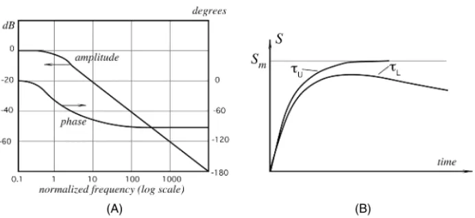
Fig. 2.9.Frequency characteristic (A) and response of a first-order sensor (B) with limited upper and lower cutoff frequencies.τuandτLare corresponding time constants.
Afirst-orderdifferential equation describes a sensor that incorporates one energy storage component. The relationship between the input s(t )and outputS(t )is the
differential equation
b1dS(t )
dt +b0S(t )=s(t ). (2.19)
A typical example of a first-order sensor is a temperature sensor for which the energy storage is thermal capacity. The first-order sensors may be specified by a manufacturer in various ways. Typical is afrequency response, which specifies how fast a first-order sensor can react to a change in the input stimulus. The frequency response is expressed in hertz or rads per second to specify the relative reduction in the output signal at a certain frequency (Fig. 2.9A). A commonly used reduction number (frequency limit) is−3 dB. It shows at what frequency the output voltage (or current) drops by about
30%. The frequency response limitfuis often called the upper cutoff frequency, as it is considered the highest frequency a sensor can process.
The frequency response directly relates to aspeed response, which is defined in units of input stimulus per unit of time. Which response, frequency or speed, to specify in any particular case depends on the sensor type, its application, and the preference of a designer.
Another way to specify speed response is by time, which is required by the sensor to reach 90% of a steady-state or maximum level upon exposure to a step stimulus. For the first-order response, it is very convenient to use a so-calledtime constant. The time constant,τ, is a measure of the sensor’s inertia. In electrical terms, it is equal
to the product of electrical capacitance and resistance:τ=CR. In thermal terms,
thermal capacity and thermal resistances should be used instead. Practically, the time constant can be easily measured. A first-order system response is
S=Sm(1−e−t /τ), (2.20)