Source Localization and Network Topology Discovery in Infection
Networks
He Hao, Daniel Silvestre, Carlos Silvestre
Abstract— Determining the network topology is typically a challenging problem due to the number of nodes and connection between them. Complexity is added whenever this identification problem relies solely on a subset of the outputs of some dynamical system or distributed algorithm running on those nodes. In this paper, we focus on both the source identification and network topology discovery problems in the context of infection networks where a subset of the nodes are elected as observers. The solution consists in writing the binary constraints associated with the problem. Convex relaxations are also proposed and investigated through simulations where a pattern emerges that placing observers in high-degree nodes increases the accuracy of the method.
I. INTRODUCTION
The network topology identification problem refers to the challenge of determining the links or connections among the various components in a network. Current research trends relating to this topic include source localization and structure discovery that that can be found in many applications in the fields of in Biology, Social Sciences, Computer and Electrical Engineering, Business, amongst others. In [1], network observability and source localization are discussed for an infection network model. The time before all nodes are infected depends on the topology, namely on the nodes degree, i.e., the number of immediate neighbors.
There is a vast body of work in the context of epidemics networks available in the literature (the interested reader is directed to a survey of traditional techniques in [2]). Typically, the initial approach is to consider a mean field approximation of the infection process and then consider what happen to the average case or the percentage of infected nodes in the network. One of the earliest works presented in [3], [4] and additional study of the threshold dividing the cases of full infection or full recovery can be found in [5]. Such models presenting the evolution of the percentage of infected nodes have attracted a lot of attention both in the continuous-time case [6] and discrete-time framework [7].
He Hao is with the Department of Electrical and Computer Engineering of the Faculty of Science and Technology of the University of Macau, Macau,
China,[email protected]
D. Silvestre is with the Department of Electrical and Computer Engineer-ing of the Faculty of Science and Technology of the University of Macau, Macau, China, and with the Instituto Superior T´ecnico, Universidade de
Lisboa, Lisboa, Portugal,[email protected]
C. Silvestre is with the Department of Electrical and Computer Engineer-ing of the Faculty of Science and Technology of the University of Macau, Macau, China, on leave from Instituto Superior T´ecnico, Universidade de
Lisboa, Lisboa, Portugal,[email protected]
This work was partially supported by the project MYRG2016- 00097-FST of the University of Macau; by the Portuguese Fundac¸˜ao para a Ciˆencia e a Tecnologia (FCT) through Institute for Systems and Robotics (ISR), under Laboratory for Robotics and Engineering Systems (LARSyS) project UID/EEA/50009/2013.
Different variants of epidemics can be found in the aforementioned literature: Susceptible-Infected (SI), Susceptible-Infected-Susceptible (SIS) and Susceptible-Infected-Recovered (SIR). Other studies such as considering nodes entering and leaving in a stochastic fashion [8] and studying the evolution from a series approximation point-of-view [9] have also been considered. Nevertheless, all these models have a shortcoming in the sense that only the macroscopic view is considered. If one would like to distinguish what happens to some individual nodes other alternatives are required.
A distinct approach present in the literature is to consider the epidemics as a group of nodes interconnected by a network that have a state indicating their current status: infected, recovered, etc. This normally entails the use of Markov Chains to model the infection process and examples can be found in [10], [11], [12], [13], [14]. These references investigate slightly different models either with self-infection links or not in order to discuss what is the threshold that leads the network to go to a full infected or disease-free state and how does the topology contributes to the transient. The markov approach is intrinsically a microscopic view that considers the individual states. A clear trade-off occurs between the two approaches in the sense that the macroscopic loses important individual information but its description is amenable whereas the microscopic view focus on the particular nodes but has an exponential state-space on the number of nodes (2n for n nodes with only two possible infected or susceptible status).
In this paper the approach is to follow the model intro-duced in [1] as a way to have a microscopic view but avoid-ing the exponential growth of the state space by introducavoid-ing a nonlinear operation on the state. The main objective is to leverage the model and make it suitable for more general discussions that we motivate for future work. Two topics are of interest, namely source localization in the infection node (discovering who was the initial infected node that caused the epidemic) and network topology identification (finding based on the measured output what is likely to be the interconnection among the various nodes). Both problems are of practical interest if we are to study an infection spreading over a network.
The subject being studied in this paper closely relates to that of Compressed Sensing where some signal is intended to be reconstructed based on a partial observation of the net-work state. In [15] the framenet-work of compressed sensing is used to retrieve the sparse network topology for a dynamical linear system. The Least Absolute Shrinkage and Selection
Operator (LASSO) have also been used in [16], [17] with a `1 penalty to ensure a sparse solution. We also use this
(now standard) penalty although the optimization function is different given that we do not have a linear model.
In [18], the approach is to design a Bayesian network to estimate the probabilities associated with each connection in the network. A similar optimization can be posed as that of constructing from data de probabilities and finding the optimal sparsest solution.
In [19] and [20], the diffusion emerges in an large scale with deterministic propagation. This spreading model has been investigated in [1] and [21], which is used to localize the source with local measurements of some states in the network. A real social network crawled from Twitter is discussed in [21] to offer an accurate rumor detection and single source identification through a greedy algorithm. The source localization process can be viewed as cardinality min-imization problem, with a standard approach to approximate the non-convex problem being an l1 minimization [22].
In this paper, we draw inspiration in this different ap-proaches and a technique applied to the discovery of the net-work structure in the aforementioned infection dynamics. We assume a propagation model where once infected/informed, the nodes remain in that state as in [1], [19] and [20]. The contributions of this paper can be summarized as:
• An extension to the diffusion model to allow for an
unknown infection time;
• A linear program based network topology discovery
algorithm for the diffusion model.
Notation: The transpose of a matrix A is denoted by A|. We
let 1n:= [1 . . . 1]|and 0n:= [0 . . . 0]|indicate n-dimension
vector of ones and zeros, and In denotes the identity matrix
of dimension n . Dimensions are omitted when no confusion arises. The vector ei denotes the canonical vector whose
components equal zero, except component i that equals one. The notation kvk1:=P
n
i=1|vi| for a vector v.
II. NETWORKMODELING ANDOBSERVABILITY
In this section, the definition for the network model is introduced along with a discussion about the observability of the problem for the particular diffusion process.
A. Modeling Diffusion
The model for the diffusion process is assumed to be a network of n components defined by the node set V := {1, 2, · · · , n} and the edge set E ⊆ V × V containing all pairs (i, j) such that there exists a connection from node i to node j. We define the adjacency matrix A ∈ Rn×n
representing the network structure corresponding to the set E. Matrix A is constructed with Aij = 1 if (i, j) ∈ E and
zero otherwise. Moreover, throughout the paper it is assumed an undirected topology which implies that A = A|.
Following the concepts in [1], a rumor or infection cannot be reversed and, therefore, the nodes are either susceptible to the infection or already infected. In the literature this definition is known as the Susceptible-Infected (SI) model. As a consequence, a single infected node at the initial time
will result in all nodes receiving the infection at a certain time in the future, provided the network is connected. The propagation is deterministic in [1], meaning that a node infected at discrete time t infects all its neighbors at t + 1.
The state of infection is denoted by the binary vector x(t) ∈ {0, 1}n. The initial state x(0) has entries equal to one
identifying the infection sources and the remaining entries equal to zero. Naturally, for a connected graph, there exists a horizon N = n−1 (i.e., equal to the largest diameter of a n-node network) such that x(N ) = 1n meaning that all nodes
were infected. The vector of measurements y(t) ∈ {0, 1}m
is a column with m elements which is obtained through the multiplication of x(t) by the m × n matrix C. Since a node cannot be infected twice, it is convenient to introduce the following notation applied to a matrix M :
Mij =
(
0, if Mij = 0
1, if Mij 6= 0
.
Given the aforementioned definitions, we recover the dynamics of the network state equation given in [1].
Theorem 1 (Diffusion Model [1]): The SI infection model is equivalent to the dynamical system modeled by the equations:
x(t) = Φ(t, 0)x(0) y(t) = Cx(t) where Φ(t, 0) = At+ At−1.
The network state equation in Theorem 1 assumes t = 0 is the initial known infection time. A generalization for Theorem 1 can be attained by considering the input vector u to inject the infection onto the source node. Dropping this assumption, we can write a new model with the state vector z(t) ∈ {0, 1}n and infection vector u(t) ∈ {0, 1}n that has
z(0) = 0. The whole model is described in the next theorem. Theorem 2 (General Diffusion Model): The SI infection model without knowledge of the initial infection is equivalent to the dynamical system defined by the following equations:
z(t) = Φ(t, 0)z(0) + t−1 X τ =0 Φ(t, τ + 1)u(τ ) y(t) = Cz(t) (1)
which can be rewritten as:
z(t) = t−1 X τ =0 Φ(t − τ − 1, 0)u(τ ) y(t) = Cz(t) (2)
Proof: In order to prove that the general diffusion model is given by (1), one has to show that (1) satisfies z(t) = x(t−tinitial), i.e., the general model is a shifted version
of the model with known initial time where tinitialis the time
where the infection was added in the general model. Consider that indeed (1) is the state equation of the system.
1 2 3 4 5 6
Fig. 1. Network Structure graph
Then, it is possible to simplify it to the format:
z(t) = Φ(t, 0)z(0) + t−1 X τ =0 Φ(t, τ + 1)u(τ ) = t−1 X τ =0 Φ(t, τ + 1)u(τ )
= Φ(t, 1)u(0) + Φ(t, 2)u(1) + ... + Φ(t, t)u(t − 1) The infection is defined as the impulse response, to the signal u, assuming node i is injected:
ui(t) =
(
1 t = tinitial
0 t 6= tinitial
Therefore, for any time t,
z(t) = Φ(t, 1)u(0) + Φ(t, 2)u(1) + ... + Φ(t, t)u(t − 1) = Φ(t, tinitial+ 1)u(tinitial)
or, equivalently,
z(t) = Φ(t − tinitial− 1, 0)u(tinitial)
by the properties of the transition matrix and thus obtaining that the model in (1) is equivalent to (2) and represents the standard model with a shifted time index of tinitial time steps.
Therefore, the format for the transition matrix in (1) becomes Φ(t, tinitial) = At−tinitial+ At−tinitial−1= Φ(t − tinitial, 0),
and the conclusion follows.
A clear advantage of the model in (1) is that it allows to envisage other possible scenarios to study under the SI model. In particular, the Susceptible Infected Recovered (SIR) model that allows for nodes to be healed or considering multiple infections outbreaks is possible in equation (1). In such cases, the signal u can have different types of values to signal when an infection appeared in the network and when a cured was applied to a specific node. The study of these models is left as a direction of future work.
B. Observability
The previous section aimed at relaxing the assumption that the initial time for the infection is known a priori. Since the source localization problem can be viewed as the state estimation of a dynamical model, one needs to discuss the observability of the system. Towards that objective, by
concatenating all the measurement information of the past N time instants, it is obtained
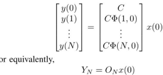
y(0) y(1) .. . y(N ) = C CΦ(1, 0) .. . CΦ(N, 0) x(0) or equivalently, YN = ONx(0)
The nm × n matrix ON reflects the characteristic of the
observers (output nodes) and is referred to as the network observability matrix. From standard observability analysis the next result is attained.
Theorem 3 (Observability [1]): If the rank of the observ-ability matrix ON is equal to n, for the particular choice of
observers, the initial state can be obtained by x(0) = (ON|ON)−1O|NYN
According to Theorem 3, when the rank of observability matrix ON is equal to n, the network is observable. As
Theorem 3 only contains the network structure and the location of the output nodes. The source localization does not depend on the initial infection time.
III. SOURCELOCALIZATION WITHOUTINITIALSTATE
INFORMATION
In the previous section, two diffusion models were pre-sented with the main difference that the external input accounts for the injection of the infection in the network.
If one assumes the strict observability condition in The-orem 3, the equation x(0) = (ON|ON)−1ON|YN provides
the exact solution. If the rank of the observability matrix is smaller than n, multiple solutions are possible and one can determine the source by finding the solution of minimal cardinality through the optimization
min x(0)
||x(0)||0
s.t. YN = ONx(0)
(3) The above l0 norm optimization attains its minimum for
the sparsest x(0) that satisfy the constraints. The l0 is not
actually a norm and is also not convex implying that the problem in (3) is an NP hard problem. However, a good approximation in practice is l1 relaxation [1]:
min x(0)
||x(0)||1
s.t. YN = ONx(0)
(4) The above is currently employed due to the fact that the l1
norm is the convex envelope of the cardinality operator. For the general model, since the initial state information is unknown, we introduce a variable size matrix O(τ ) that cor-responds to observability matrix for the first τ observations of the general model as
O(τ ) = C CΦ(1, 0) .. . CΦ(τ, 0)
which is the same definition for the observability matrix but with the notation O(τ ) to make it clear that we are writing a condition that has to be evaluated for different values of τ . Furthermore, from Theorem 2, we have z(t) = Pt
τ =1Φ(t, τ )u(τ ), meaning that τ is the only variable
determining the matrix O(τ ) and the state of the infection network for each time instant. Therefore, if we choose a particular τ?, the matrix O(τ?) is constant and we can write
Yτ= Oτ?u(τ ), where clearly the variable size matrix O(τ )
is a fixed size matrix Oτ?for that particular choice τ?. Then,
(4) becomes
min u(τ )
||u(τ )||1
s.t. Yτ = O(τ )u(τ ).
The above formulation essentially seeks to solve the source localization with unknown initial time information by testing each possible τ value that corresponds to the tinitial of that
infection. Nevertheless, all the optimization problems can be casted together in the following manor:
min u ||u||1 s.t. Yt= Otu
(5) where Ytstacks all available measurements from time instant
one up until the current time instant, the variable u is of size nt × 1 and gathers the variables u(0), u(1), · · · , u(t − 1) and the observability matrix is given by
Ot= CΦ(1, 1) 0 · · · 0 CΦ(2, 1) CΦ(2, 2) · · · 0 .. . ... . .. 0 CΦ(t, 1) CΦ(t, 2) · · · CΦ(t, t) .
The formulation in (5) seeks to find the sparsest set of inputs u(0), · · · , u(t − 1) such that all constraints given by the measurements are validated. Remark that one could add a set of weights to be multiplied by the vector u as to favor solutions where the entries equal to one in that vector appear in the beginning. Nevertheless, such tricks might not be beneficial and the solver might output non-sparse vectors.
IV. NETWORKSTRUCTUREDISCOVERY
In this section, we focus on determining the uncertain network topology from the known infection source and observers. The assumption is that the network designer can arbitrarily place infected nodes and take measurements for the set of observers in order to construct from that output the network topology.
Under the aforementioned assumptions, the model in The-orem 1 is suitable for the task of discovering the network topology. Given the selected choice for initial infected node, the equation
YN = ONx(0)
allows to place some constraints on the network topology. The matrix P represents the unknown adjacency matrix. Given that each entry is either 0 or 1 it naturally induces a Boolean Satisfiability problem. The objective of this section
is to reformulate and obtain a convex approximation of such problem.
Given that the network is undirected, P is symmetric and also self-cycles are not possible in the context of our problem, leading to
Pii= 0, ∀1 ≤ i ≤ n.
Defining ON using the matrix P instead of A, each of the
rows in ON represents a boolean clause that we denote by
α`, 1 ≤ ` ≤ mN (there are N time instants each producing
a matrix with m rows). Consider the network in Fig. 1 as an example and assume that node 1 was infected and nodes 3, 4 and 5 are selected as observers. The measurement y(0) = 03
has no information apart from the fact that the infected node is not one of the observers making α1, α2 and α3 clauses
with no information, i.e., the logical value of 1 (indeed this are removed by any solver). The measurement y(1) = e1
allows to write α4, α5 and α6 with some meaning. First,
computing CΦ(1, 0)x(0) = P13 P14 P15 , Φ(t, 0) := Pt+ Pt−1
determines that α4 = P13, α5 = ¬P14 and α6 = ¬P15,
where the symbol ¬ stands for the logical negation. In doing so, the various clauses α` establish the set of possible
instantiations for the variables Pij representing the existence
or not of a link in the network.
The network discovery problem can then be casted as that of the solution of a satisfiability problem (SAT) in conjunc-tive normal form α1∧ α2∧ · · · ∧ αmN. The SAT problem
has been extensively studied in the literature, but given that it is combinatorial by nature, its complexity increases expo-nentially. Nevertheless, the SAT problem can be equivalently formulated as an optimization problem as:
min P 1 s.t. AVEC(P ) >= β, Pii = 0, 1 ≤ i ≤ n, P = P|, Pij = 0 ∨ Pij= 1, i 6= j (6)
where A is built from the α` variables by placing 1 if the
corresponding Pij variable appears and −1 if it appears with
the logical negation, β is a vector equal to one minus the number of variables appearing negated and VEC(P) is the vectorization operator that we assume to vectorize only the lower triangular part of P since P is symmetric. As an example, if there was only three clauses P14, P12∨ ¬P13
and ¬P23 ∨ ¬P12 in a four node network, the constraint
AVEC(P ) >= β would be characterized by:
0 0 1 0 0 0 1 −1 0 0 0 0 −1 0 0 −1 0 0 P12 P13 P14 P23 P24 P34 >= 1 0 −1 .
Number of Observers 1 2 3 4 5 6 Successful Runs 0 100 200 300 400 500 600 700 800 900 1000
With Initial Infection Information Without Initial Infection Information
Fig. 2. Number of successful initial infection localizations.
Remark that the optimization problem in (6) is just testing the feasibility of a solution and that the only source of non-convexity is the constraint that the entries in P are either zero or one. One of the common approach is to relax such assumption to the convex approach of 0 ≤ Pij ≤ 1.
In particular, if one wants to find the sparsest network topology that is feasible obtains the whole optimization problem min P 1 | nP 1n s.t. A VEC(P ) >= β, Pii= 0, 1 ≤ i ≤ n, P = P|, 0 ≤ Pij ≤ 1, i 6= j
which is convex and a linear program. Notice that we have not used the `1 norm since all Pij >= 0 so there is no
need to apply the absolute value operator and also because the norm would not ensure the sparsest solutions for cases where one of the nodes is fully connected (or is of higher degree then the rest).
V. SIMULATIONRESULTS
In this section, we provide simulations to illustrate the proposed algorithms in this paper. The first simulation com-pares the accuracy of the source localization between the two cases. The setup includes a randomly selected network topology for n = 6 where both models are simulated with the number of observers ranging from one to six. In order to have challenging cases, the random network generation works by either introducing each possible link or not with a 0.5 probability. This means that on average half of the possible links are going to be added. The experiment is reproduced in a 1000 monte carlo run and the aggregate successful recovery of the initial infection is presented in Fig. 2.
From the simulation results, we can find a common characteristic of these two models that with the increase of observers, there are more successful runs. As expected the general model has a smaller accuracy but is broader in terms of application.
To further see the emerging trend refer to the 3 where the difference in the success rate between the two models is
Number of Observers 1 2 3 4 5 6 Success Percentage 0 0.05 0.1 0.15
Success Rate Difference
Fig. 3. Difference between the success rate of the two considered models.
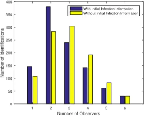
Number of Observers 1 2 3 4 5 6 Number of Identifications 0 50 100 150 200 250 300 350 400
With Initial Infection Information Without Initial Infection Information
Fig. 4. Number of successful infection identification depending on the
minimum number of required observers for 1000 monte carlo run.
depicted.
In Fig. 3 it is presented the loss in source localization success rate. The value decreases close to a linear fashion from about 0.14 to 0.02 when considering 2 to 5 observers, while the difference in the cases of having 1 and 6 observers are similar. One possible reason for the loss in initial infection detection is that more configurations of infection can justify the measurements in the general model.
In order to achieve a better understanding of the general model, a new simulation was performed for a 1000 monte carlo runs using random network structures. In this setup, instead of running the models for different values of the number of observers, the models are run for one observer and it is increases only if the localization is unsuccessful. The final value for the number of observers that achieved the recovery of the initial infection is presented in Fig. 4.
Figure 4 indicates that close to 150 of the 1000 network topologies allowed the source localization with just one observer when knowing the initial time in comparison to 100 out of 1000 for the general model. Once again, a loss of recovery efficacy is found for the general model as the extra degree of freedom means that there might be different initial injections that account for the same output sequences. One of the main future objectives is to find out if the accuracy can be improved using different approximation techniques of the non-convex problem.
The network structure discovery when considering the infection model with initial information is also presented in
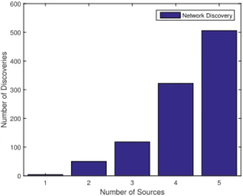
Number of Sources 1 2 3 4 5 Number of Discoveries 0 100 200 300 400 500 600 Network Discovery
Fig. 5. Number of successful network discoveries depending on the
minimum number of required observers for the monte carlo run.
this paper. In this setup, 1000 monte carlo runs are used to test the algorithm of discovering the randomly generated network topology. For that purpose, in each experiment the number and location of the observers is fixed and the process is run with an initial infection. If the optimization procedure returns a solution P composed of zeros and ones the algorithm halts. Otherwise, it tests one of the remaining nodes to be the initial infection. The least number of sources needed to determine the network is shown in Fig. 5. For one thousand random network structures, about half of them need to have 5 different sources being injected into the network. A critical key influence in the need to have 5 infection processes to half of the topologies is a consequence of the random network generations that is creating high-degree networks with nodes having on average half of the nodes as neighbors. The intuition behind this choice was that the best case scenario would be the path graph since the infection of one of the single-neighbors nodes would lead to detection as opposed to the complete network where n − 1 infections are required (in each infection process the solvers learns that the current initial node is connected to all the others but no information regarding the connections between the remaining nodes).
VI. DISCUSSION ANDFUTUREWORK
In the paper, we have presented an extension to the Susceptible-Infected (SI) model in its dynamical system view. In particular, by allowing an unknown initial infection time. The source localization and network discovery via convex relaxations are investigated.
In simulations, we have found the loss of accuracy to be below 15% which is encouraging given the possibilities of the general model. Half of the network as observers allowed to identify the location in 60% for random networks with n/2 connectivity. All randomly generated networks were successfully discovered by the procedure proposed herein.
As directions of future work, two main trends can be pursued: use the general model framework to show how more evolved methods for infection networks can be simulated (for example the Susceptible-Infected-Recovered, SIR, model); and, investigated algorithms to select the sequence of initial infections that render a faster network topology discovery.
REFERENCES
[1] S. Zejnilovi, J. Gomes, and B. Sinopoli, “Network observability and localization of the source of diffusion based on a subset of nodes,” in 51st Annual Allerton Conference on Communication, Control, and Computing (Allerton), Oct 2013, pp. 847–852.
[2] M. J. Keeling and K. T. Eames, “Networks and epidemic models,” Journal of The Royal Society Interface, vol. 2, no. 4, pp. 295–307, 2005.
[3] J. O. Kephart and S. R. White, “Directed-graph epidemiological models of computer viruses,” in IEEE Computer Society Symposium on Research in Security and Privacy, May 1991, pp. 343–359. [4] ——, “Measuring and modeling computer virus prevalence,” in IEEE
Computer Society Symposium on Research in Security and Privacy, May 1993, pp. 2–15.
[5] D. Chakrabarti, Y. Wang, C. Wang, J. Leskovec, and C. Faloutsos, “Epidemic thresholds in real networks,” ACM Transactions on Infor-mation and Systems Security, vol. 10, no. 4, pp. 1:1–1:26, Jan. 2008. [6] Y. Moreno, R. Pastor-Satorras, and A. Vespignani, “Epidemic out-breaks in complex heterogeneous networks,” The European Physical Journal B - Condensed Matter and Complex Systems, vol. 26, no. 4, pp. 521–529, Apr 2002.
[7] L. J. Allen, “Some discrete-time SI, SIR, and SIS epidemic models,” Mathematical Biosciences, vol. 124, no. 1, pp. 83 – 105, 1994. [8] J. A. Jacquez and C. P. Simon, “The stochastic SI model with
recruitment and deaths I. comparison with the closed SIS model,” Mathematical Biosciences, vol. 117, no. 1, pp. 77 – 125, 1993. [9] H. Khan, R. N. Mohapatra, K. Vajravelu, and S. Liao, “The explicit
series solution of SIR and SIS epidemic models,” Applied Mathematics and Computation, vol. 215, no. 2, pp. 653 – 669, 2009.
[10] P. Van Mieghem, “The N-intertwined SIS epidemic network model,” Computing, vol. 93, no. 2, pp. 147–169, Dec 2011.
[11] P. Van Mieghem and E. Cator, “Epidemics in networks with nodal self-infection and the epidemic threshold,” Physics Review E, vol. 86, p. 016116, Jul 2012.
[12] A. Ganesh, L. Massoulie, and D. Towsley, “The effect of network topology on the spread of epidemics,” in IEEE 24th Annual Joint Conference of the IEEE Computer and Communications Societies., vol. 2, March 2005, pp. 1455–1466 vol. 2.
[13] S. Gmez, A. Arenas, J. Borge-Holthoefer, S. Meloni, and Y. Moreno, “Discrete-time markov chain approach to contact-based disease spreading in complex networks,” Europhysics Letters, vol. 89, no. 3, p. 38009, 2010.
[14] P. Van Mieghem, J. Omic, and R. Kooij, “Virus spread in networks,” IEEE/ACM Transactions on Networking, vol. 17, no. 1, pp. 1–14, Feb. 2009.
[15] D. Hayden, Y. H. Chang, J. Goncalves, and C. J. Tomlin, “Sparse network identifiability via compressed sensing,” Automatica, vol. 68, pp. 9 – 17, 2016.
[16] A. J. Seneviratne and V. Solo, “Topology identification of a sparse dynamic network,” in 51st IEEE Conference on Decision and Control (CDC), Dec 2012, pp. 1518–1523.
[17] B. M. Sanandaji, T. L. Vincent, and M. B. Wakin, “Exact topology identification of large-scale interconnected dynamical systems from compressive observations,” in American Control Conference, June 2011, pp. 649–656.
[18] A. Chiuso and G. Pillonetto, “A bayesian approach to sparse dynamic network identification,” Automatica, vol. 48, no. 8, pp. 1553 – 1565, 2012.
[19] P. C. Pinto, P. Thiran, and M. Vetterli, “Locating the source of diffusion in large-scale networks,” Physical Review Letters, vol. 109, p. 068702, Aug 2012.
[20] D. Shah and T. Zaman, “Rumors in a network: Who’s the culprit?” IEEE Transactions on Information Theory, vol. 57, no. 8, pp. 5163– 5181, Aug 2011.
[21] Identifying rumors and their sources in social networks, vol. 8389, 2012.
[22] D. L. Donoho, “For most large underdetermined systems of linear equations the minimal l1-norm solution is also the sparsest solution,” Communications on Pure and Applied Mathematics, vol. 59, no. 6, pp. 797–829, 2006.