Projeto de redes Ad Hoc sem fio ciente de topologia

PROJETO DE REDES AD HOC SEM FIO CIENTE DE

TOPOLOGIA

Tese apresentada ao Programa de Pós--Graduação em Ciência da Computação do Instituto de Ciências Exatas da Uni-versidade Federal de Minas Gerais como requisito parcial para a obtenção do grau de Doutor em Ciência da Computação.

O

RIENTADOR

: A

NTONIO

A

LFREDO

F

ERREIRA

L

OUREIRO

C

OORIENTADOR

: A

LEJANDRO

C

ESAR

F

RERY

O

RGAMBIDE

Belo Horizonte

TOPOLOGY-AWARE DESIGN OF WIRELESS AD HOC

NETWORKS

Thesis presented to the Graduate Pro-gram in Computer Science of the Univer-sidade Federal de Minas Gerais in partial fulfillment of the requirements for the degree of Doctor in Computer Science.

A

DVISOR

: A

NTONIO

A

LFREDO

F

ERREIRA

L

OUREIRO

C

O

-

ADVISOR

: A

LEJANDRO

C

ESAR

F

RERY

O

RGAMBIDE

Belo Horizonte

Ramos Filho, Heitor Soares

R175p Projeto de redes ad hoc sem fio ciente de topologia

/Heitor Soares Ramos Filho. — Belo Horizonte, 2012 xxvi, 187 f. : il. ; 29cm

Tese (doutorado) — Universidade Federal de Minas Gerais. Departamento de Ciência da Computação.

Orientador: Antonio Alfredo Ferreira Loureiro. Coorientador: Alejandro Cesar Frery Orgambide.

1. Computação Teses. 2. Redes de computadores -Teses. 3. Sistemas de comunicação sem fio - -Teses. I. Orientador. II. Coorientador. III. Título.

Foremost, I am grateful to my wife. Karina, thank you for being part of my life, specially during this long and hard journey that culminated with this thesis. We did this together. I have no words to express all love, companionship, support, and everything we are having together. Thanks for everything.

I would like to express my sincere gratitude to my parents that not only gave me birth, but provided me the opportunity of having a solid education. They are my main reference of ethnics, politeness and moral. Thanks for always being such great parents. I also would like to extend my gratitude to all family members that always encouraged me to overcome all challenges posed by this PhD.

I take this opportunity to record my sincere thanks to my advisor and friend Loureiro. I am extremely grateful for his expert, sincere and valuable guidance. He masters the art of encouragement. He is always very positive and optimistic. More often than not he was much more upbeat and confident with my work than me. Thanks for all valuable technical discussions, guidance, advices, and a special thanks for all many opportunities you offered me during this process. Thanks for trusting me for all those challenging missions.

I also would like to thank my co-advisor and great friend Alejandro. We are long-term partners since he was my master’s advisor. I have no words to

Thanks for all support.

I also take this opportunity to thanks my mentor during my internship at Microsoft Research, Jie. For me, this internship was much more than a simple internship mostly because Jie did such a great job supervising me. He set the bar high and guided me to reach great goals. I could not expect to reach such great achievements in a job of only three months. Special thanks to Bodhi, also from MSR, for all valuable collaboration on this work.

My sincere gratitude to Azzedine Boukerche that supervised me during the period I spent in the Paradise Laboratory at the University of Ottawa, Canada. Thanks for accepting me as an exchange student and for supporting me.

During this journey I had the pleasure of meeting and interacting with many people that now I can proudly call friends. They made my journey easier and we spent good times together. Especial thanks for guys from UFMG, Paradise laboratory at uOttawa, and Microsoft Research. All those guys had an intense participation on this journey, some of them I had the opportunity to have some collaboration and some others I had the pleasure to be a friend. I want to record a special thank to the guys I had the opportunity to scientifically collaborate like Richard, Leandro, Eduardo Muccelli, Guidoni, Nakamura, Cristiano, Renfei, Tao, Aman, Bodhi, Ted, and Felipe.

I would like to record a special thank for the guys from the tennis team of Alta Energia in Belo Horizonte. I had a great pleasure playing tennis with them. They made a great effort trying to improve my tennis skills (poor guys).

I also would like to be grateful to the staff of Computer Science department for all support. Special thanks to Renata, Sheila, Túlia and Maristela.

(Leonardo Da Vinci)

Neste trabalho, estudamos a relação entre métricas topológicas no contexto de redes Ad Hoc sem fio e medidas de desempenho da rede. Neste contexto, estamos interessados na aplicação de diferentes conceitos e métricas relacionadas com a topologia da rede em três modelos de redes distintos: (i) redes de sensores sem fio (WSNs), (ii) redes móveis sem fio (MANETs) e, (iii) redes ad hoc veiculares (VANETs). Esses três modelos cobrem uma grande variedade de topologias, que apresentam diferentes características, desde as WSNs típicas, que não apresen-tam mobilidade (ou apresenapresen-tam baixa mobilidade), até redes alapresen-tamente dinâmi-cas como as VANETs. As principais contribuições alcançadas são: primeiramente, foi proposto um modelo expressivo de topologias para redes de sensores sem fio, que é apto a descrever uma grande quantidade de estratégias de deposição de nós. Neste contexto, foi proposta uma métrica topológica baseada no betwee-ness que é capaz de representar o consumo de energia relacionado à tarefa de retransmissão de dados em WSNs. Também foi apresentado um algoritmo dis-tribuído que calcula essa métrica. Esse algoritmo foi utilizado no projeto de um protocolo de roteamento que balanceia o trabalho de retransmissão de dados, aumentando o tempo de vida da rede. No contexto de MANETs, foi desenvolvido um método de localizacão de nós baseado em GPS que transfere os dados brutos do sinal de GPS para uma plataforma de nuvem, reduzindo o consumo de energia

cional. Para o caso de redes que apresentam alta mobilidade como as VANETs, foi proposta a utilização de técnicas de rastreamento cooperativo para acompanhar as rápidas mudanças de topologia ocasionadas pela alta velocidade dos veícu-los. Essa solução foi utilizada para aumentar o desempenho de mecanismos de distribuição de vídeo em VANETs.

In this work, we study the relationship between topological metrics of Wireless Ad Hoc Networks and the network performance. We are interested in applying different concepts and metrics related to the network topology to three differ-ent network models, namely (i) wireless sensor networks (WSNs), (ii) mobile ad hoc networks (MANETs), and (iii) vehicular ad hoc networks (VANETs). These three models cover a wide variety of network topologies, ranging from typically static or nearly static topologies (WSNs) to highly dynamic topologies such as the ones present in VANETs. The main contributions of this work are: firstly, we pro-pose an expressive topology model able to describe a wide variety of deployment strategies for WSNs. We present a topology-related feature estimator derived from the betweenness metric, suitable for representing the energy depletion re-lated to the sensor relay task in WSNs. We developed a distributed algorithm to compute this metric, which was used to design a routing algorithm that aims to make a fair balance of the relay task of nodes in a WSN. For MANETs, we de-veloped a new localization system for Internet capable devices, based on A-GPS technology, which offloads the GPS raw signal data to the cloud. We show that this technique is able to reduce the energy consumption up to 80% when com-pared to traditional A-GPS. To tackle with the highly dynamic topologies present in VANETs, we proposed the use of a cooperative target tracking solution to track

VANETs.

1.1 Wireless networks models . . . 2 1.2 Topology-aware ad hoc node components . . . 5

2.1 Outcomes of M2P2for 300 nodes with 1, 10, 10 and 15 H-sensors (in black) and attractiveness 15, 5, 10 and 15, respectively . . . 19 2.2 Two outcomes of network graphs generated by the M2P2model. Dark

points are the H-sensors, gray points are the L-sensors and the triangle is the sink node . . . 20 2.3 Comparison of Q-model and M2_P2 _{. . . . 21}

2.4 Three different wireless channel models . . . 26 2.5 Correlation between spent energy and measures of centrality, simple

gossip routing and URP deployment . . . 32 2.6 Corrrelograms and scatterplots for gossip routing and URP

deploy-ment, 100 and 400 nodes, centered (C) and randomly (R) placed sink 33 2.7 Correlation between spent energy and measures of centrality, random

tree routing and URP deployment . . . 34 2.8 Corrrelograms and scatterplots for tree routing and URP deployment,

100 and 400 nodes, centered (C) and randomly (R) placed sink . . . 35

2.10 Corrrelograms and scatterplots for gossip routing, Q-Model, 100 and 400 nodes, centered placed sink . . . 38 2.11 Correlation between spent energy and measures of centrality, tree

routing and Q-Model deployment . . . 39 2.12 Corrrelograms and scatterplots for tree routing and Q-Model, 100 and

400 nodes, centered placed sink . . . 40 2.13 Coverage and connectivity as a function of the number of H-sensors 45 2.14 Clustering coefficient and the average path length . . . 46 2.15 Energy consumption metrics as function of the number of H-sensors . 49

3.1 Examples of Betweenness and SBet values for two sink positions, cen-ter and corner and their respective histograms (the sink is represented by the triangle) . . . 65 3.2 Node A is more central than node B in terms of number of shortest

paths to the sink (the pentagon at the center) . . . 66 3.3 An illustrative network with sink (pentagon) and sensors (circles, and

lozenges). For each sensor, we have the SBet value within parenthe-ses, and number of paths from the sink within brackets. The circular-shaped sensors have the Relay role, while the lozenges have the Bor-der role. . . 70 3.4 Average number packets sent per node upon the hop level . . . 74 3.5 Percentage of transmitted messages as a function of the hop distance 76 3.6 Uneven distribution of transmissions for nodes located one hop from

the sink . . . 77 3.7 Relay selection decision rule . . . 79 3.8 Behavior of the randomSbetTree algorithm upon varying the

param-eter T . . . 83 3.9 Analysis of the number of transmissions . . . 85 3.10 Max number of transmissions upon varying the number of nodes . . . 86 3.11 IQR of transmissions upon varying the number of nodes . . . 87 3.12 Relative entropy of transmissions upon varying the number of nodes 88

4.3 Navigational data: one frame composed by six sub-frames . . . 100

4.4 Instantaneous power consumption for acquisition phase . . . 108

4.5 Instantaneous power consumption for acquisition, tracking and posi-tion calculaposi-tion phases . . . 109

4.6 Solution ambiguity . . . 111

4.7 The flow of CO-GPS backend web service. . . 112

4.8 The GSP data collector used for experiments . . . 113

4.9 Duty cycling in experimental evaluation. After an idle period (called a gap), the receiver collects a chunk of raw data. . . 115

4.10 The number of acquired satellites in various experiment settings. . . . 116

4.11 Location error distribution in various experiment settings when single chunk is used for location calculation . . . 117

4.12 Overall location accuracy distribution. . . 119

4.13 Overall results from 6 locations. The shadow is 100m in diameter. We see that there are bias errors in some cases. . . 121

4.14 Error due to time drift . . . 122

4.15 Energy savings from CO-GPS mode in two representative scenarios. . 125

5.1 Cooperative target tracking scenarios . . . 132

5.2 Basic components of cooperative target tracking systems . . . 134

5.3 Non-linear relation between sensor and Cartesian coordinations system139 5.4 Data association problem . . . 141

5.5 Forwarding zone . . . 150

5.6 Example of multi-modal hypothesis for vehicular state estimation . . 153

5.7 Frame loss . . . 159

5.8 Delay . . . 160

5.9 Cost . . . 161

2.1 Simulation scenarios used in the SBet energy analysis . . . 28

2.2 Simulation scenarios used in the M2_P2 _{model analysis . . . . 42}

2.3 Small world characterization of the M2_P2_{model . . . . 47}

3.1 Description of variables used in Algorithms 1, 2 and 3 . . . 67

3.2 The content ofBorderpacket fieldsonsPaths, andψset for each node of the network shown in Figure 3.3 . . . 71

3.3 Necessary overhead to calculate the SBet metric . . . 73

3.4 Simulation scenarios used in the randomSbetTree algorithm analysis 81 4.1 Summary of A-GPS assistance for different type of starts . . . 103

4.2 Scenarios of evaluation for CO-GPS . . . 115

4.3 Error statistics . . . 120

5.1 Summary of motion models . . . 138

5.2 Solutions parameters . . . 158

Acknowledgments ix

Resumo xiii

Abstract xv

List of Figures xvii

List of Tables xxi

1 Introduction 1

1.1 Motivation . . . 1 1.2 Goals . . . 5 1.3 Contributions . . . 6 1.4 Outline . . . 7

2 Modeling and characterization of WSNs 9

2.1 Introduction . . . 10 2.2 Related work . . . 12 2.3 Topology model: the M2P2process . . . 15

2.4 Topological characterization: the sink betweenness measure . . . . 22 2.4.1 Centrality metrics . . . 22 2.4.2 Evaluation models in the SBet energy analysis . . . 24 2.4.3 Evaluation scenarios used in the SBet analysis . . . 28 2.4.4 Results . . . 29 2.5 Evaluation of the M2_P2 _{model . . . . 38}

2.5.1 Coverage and connectivity . . . 43 2.5.2 Small world characterization . . . 44 2.5.3 Energy balancing . . . 48 2.6 A guide to a stochastic planned deployment . . . 50 2.7 Chapter remarks . . . 52

3 Topology-aware design of WSNs 55

3.1 Introduction . . . 56 3.2 Related work . . . 58 3.2.1 Topology-related algorithms . . . 58 3.2.2 Energy hole . . . 60 3.2.3 Load balance in WSNs . . . 61 3.3 Sink betweenness and wireless sensor networks . . . 62 3.4 Distributed algorithm for sink betweenness . . . 66 3.4.1 Node initialization . . . 69 3.4.2 Dealing with the Hello packet . . . 69 3.4.3 Sending the border packet . . . 69 3.4.4 Dealing with the border packet and calculating SBet . . . . 69 3.4.5 Analysis . . . 71 3.5 Sink betweenness and energy hole . . . 75 3.5.1 Methodology . . . 75 3.5.2 Evaluation . . . 79 3.5.3 Results . . . 82 3.5.4 Summary of the results . . . 87 3.6 Chapter remarks . . . 89

4.2 GPS basics . . . 93 4.2.1 GPS signal . . . 94 4.2.2 GPS receiver . . . 96 4.2.3 Navigation equations . . . 99 4.2.4 A-GPS . . . 102 4.2.5 Coarse time navigation . . . 103 4.2.6 GPS energy . . . 106 4.3 Our proposal . . . 108 4.3.1 Web services . . . 111 4.3.2 Evaluation . . . 113 4.3.3 Acquisition quality . . . 114 4.3.4 Location accuracy . . . 118 4.3.5 Time accuracy . . . 120 4.3.6 Energy consumption . . . 123 4.4 Related work . . . 125 4.5 Chapter remarks . . . 126

5 Cooperative target tracking in Vanets 129

5.1 Introduction . . . 130 5.2 Problem statement . . . 133 5.3 Components of cooperative target tracking systems . . . 133 5.3.1 Motion models . . . 135 5.3.2 Measurements . . . 138 5.3.3 Data association . . . 140 5.3.4 Communication . . . 142 5.3.5 Filtering . . . 144 5.4 Case study: data dissemination in VANETs . . . 147 5.4.1 CTT-based data dissemination algorithm . . . 148 5.4.2 Target tracking mechanism . . . 151 5.4.3 Performance evaluation . . . 155 5.5 Related work . . . 161

6 Final remarks 165

6.1 Conclusions and outlook . . . 165 6.2 Publications . . . 168 6.2.1 Periodicals . . . 168 6.2.2 Conferences . . . 169 6.2.3 Under Submission . . . 170 6.2.4 Short Course . . . 171 6.2.5 Awards . . . 171

Bibliography 173

1

Introduction

“Great things are not done by impulse, but by a series of small things brought together”

Vincent van Gogh

✶✳✶ ▼♦t✐✈❛t✐♦♥

Wireless networks consist of a set of nodes that communicate through wireless channels. There are different kinds of wireless networks such as wireless personal area networks (WPAN), wireless local area networks (WLAN), wireless mesh net-works (WMESH), wireless metropolitan area netnet-works (WMAN), wireless wide area networks (WAN) and cellular networks. Those networks are characterized mainly by the network range. For instance, WPANs typically connect few de-vices that span a relative small area within a person’s reach. Conversely, cellular networks connect a large number of mobile devices (mobile phones) and span large areas such cities, continents and even devices in different continents. The challenges to interconnect the devices in each of those networks change abruptly because their characteristics are diverse.

Infrastructured Wireless

Network Ad Hoc Wireless Networks

Figure 1.1: Wireless networks models

Some wireless networks require an established infrastructure to work prop-erly. This is the typical case of WLANs where desktop computers, laptops, print-ers, and other devices connect to an access point to share services. The same situation occurs in cellular networks where the cell towers act as an access point, and are responsible for connecting a limited number of devices within a limited area. Access points may be interconnected, so, devices that are connected to a different access points may be able to communicate. Those networks are heavily dependent on the infrastructure. For example, in the case of a failure in an ele-ment of the infrastructure, all devices attached to it are not able to communicate even if they are in the range of other devices.

phones and WLAN devices are connected by an access point. On the right side, we can observe three well-known wireless ad hoc networks: wireless sensor net-works (WSN), mobile ad hoc netnet-works (MANET) and vehicular ad hoc netnet-works (VANET). Some devices can also work in a hybrid mode, i.e., they work attached to an access point but are able to communicate in ad hoc mode. In this thesis, we are mostly interested in wireless ad hoc networks.

In such networks, the nodes are usually randomly deployed in the workspace. For instance, wireless sensor nodes are typically launched onto a region of interest. MANETs are formed by nodes that move around and form ran-dom topologies. The same situation happens in VANETs where vehicles are con-nected by chance while moving around. Thus, stochastic point processes[ Badde-ley, 2006; Baccelli, 2009]theory describes the location of a number of points in a region of the space, and is a natural way of representing the random nature of ad hoc networks nodes’ location. Nodes are able to communicate only when they are into the communication range of each other. Thus, the network connectiv-ity induces a particular case of random graph [Erd˝os and Rényi, 1959], namely geographic random graphs.

The topology induced by network connectivity plays an important role in the design and the operation of wireless ad hoc networks. Many properties like coverage, connectivity, lifetime and network congestion are directly influenced by the way nodes are placed in the workspace. For instance, in a WSN scenario, Younis and Akkaya[2008]suggest that the deployment can be optimized in func-tion of area coverage, network connectivity, network longevity and data fidelity. Moreover, Hoydis et al.[2009]present a study on the effects of the topology on local throughput capacity of medium access protocols in the context of ad hoc networks. They concluded that the way nodes are deployed has strong impact on the local throughput, which is related to network capacity and performance. They point to the need of more complete studies involving different deployment strategies beyond the usual random deployment.

Celebi and Arslan[2007]proposed a location-aware engine architecture for cognitive wireless radio and networks. Their studies unveil that location infor-mation can be used to optimize the network performance. Hoydis et al. [2009]

neighbor-hood information can be used to improve performance. They also stated that further work is called for, i.e., there are open research venues involving the rela-tionships between topology and network characteristics. Their studies are only related to the relationship of throughput and topology.

Haenggi et al. [2009] present a study of the modeling of random nodes location by, for instance, a Poisson point process. They argued that stochastic geometry and random graph theory are indispensable tools for the analysis of wireless networks, and that such tools lead to analytical results on a number of important problems. For instance, they apply those techniques to model and quantify interference, connectivity, outage probability, throughput, and capacity of wireless networks deployed as Poisson point process.

Perillo and Heinzelman [2009] proposed several coverage-aware routing protocols to route traffic around sparsely deployed regions so that the coverage remains high for a long lifetime. Their proposal intends to increase the over-all lifetime of the network by avoiding the sparsely sensed regions. A carefully study of that work reveals that routing metrics based on coverage properties are, actually, based on topology metrics (node density).

The aforementioned studies illustrate the importance of the topology in wireless ad hoc networks. This thesis is situated in this context, and is focused on the following research subjects: (i) the identification of topological informa-tion/metrics relevant to the design and operation of wireless ad hoc networks, (ii) the estimation of the topological information/metric of interest, and (iii) the design of topology-aware algorithms that take advantage of topological informa-tion to improve the network performance.

Wireless Ad Hoc Node Topology

Inference Module

Network Protocol Stack

Physical Devices Sensors

Figure 1.2: Topology-aware ad hoc node components

✶✳✷ ●♦❛❧s

✶✳✸ ❈♦♥tr✐❜✉t✐♦♥s

The main contributions of this thesis are:

M2_P2_{: a topological model for WSNs: that network is a special type of an ad}

hoc network where autonomous devices cooperatively monitor a set of observable phenomena. We propose the Multilevel Marked Point Process M2P2, an expressive model able to represent a wide variety of WSNs scenar-ios, from totally random to planned stochastic node deployment in wireless sensor networks. This model can be easily included in any simulation plat-form for WSNs.

SBet: a novel centrality metric tailored for WSNs: a centrality metric derived

from betweenness, namely Sink Betweeness, SBet for short. We showed that SBet is more suitable for representing WSN characteristics and that it is highly correlated with the energy spent in the relay task of a node in a WSN. Thus, both, M2_P2 _{and Sbet are powerful tools on the design space}

of WSNs. A designer, will be able, for instance, to evaluate how many nodes should be deployed, how many low- and high-end nodes (nodes with more powerful battery and communication radius) should be deployed to increase the network lifetime. SBet can also be used to design topology-aware algorithms that benefits from the knowledge of this metric in order to improve the network performance.

CO-GPS: a low energy GPS-based localization for MANETs: location is one of

A cooperative target tracking module for VANETs: a module that accommo-dates all necessary features for tracking targets in vehicular networks. Tar-get tracking plays a key role for vehicular ad hoc networks (VANETs) due to the fact that a wide variety of envisioned applications rely on the ability of detecting, localizing and tracking objects (for instance, other vehicles) surrounding a given vehicle. Thus, vehicles are able to manage the highly dynamic topologies present in this kind of network by tracking the state (localization, velocity, acceleration, etc) of surrounding nodes.

CTTDD: a location-aware multimedia data dissemination for VANETs: a

data dissemination scheme for VANETs, namely Cooperative Target Track-ing based Data Dissemination algorithm (CTTDD), that takes advantage of the target tracking module. In our approach, the nodes only store the states of the neighbors that are directly involved in the data communica-tion process. Our algorithm uses the neighbors’ locacommunica-tion and near-future predictions to drive the relay selection process.

✶✳✹ ❖✉t❧✐♥❡

2

Energy-aware topology

modeling and characterization

of wireless sensor networks

“All our knowledge has its origins in our perceptions”

Leonardo da Vinci

Heterogeneous wireless sensor networks were proposed to address some fundamental limits and performance issues present in homogeneous Wireless Sensor Networks (WNS). The use of a set of high-end sensors may lead to in-crease some WSNs capabilities in different ways. Thus, the network can be comprised, for instance, of two different set of nodes, namely low- and high-end nodes (L- and H-sensors, respectively). High-high-end nodes usually present higher battery capacity and higher transmission ranges (more powerful radio), while low-end nodes are regular WSN nodes. Questions as, for instance, how many high-end sensors should be used and how to plan their deployment need a proper assessment. In this work, we propose a novel modeling solution that is able to represent a wide variety of scenarios, from totally random to planned stochastic node deployment in heterogeneous sensor networks. This model en-compasses homogeneous and heterogeneous networks showing characteristics of small-world networks and can address the energy hole problem. We show that using only about 3 % of high-end sensors and deploying nodes by using the

slightly attractive model herein defined, we observe improved characteristics of the network topology, among them: (i) low average path length, (ii) high cluster-ing coefficient and (iii) fairly relay task distribution among the sensors. We also provide a comprehensive guide of how to deploy nodes to improve the lifetime by diminishing the energy hole effect by using topological metrics. Moreover, we evaluate a topological metric, namely Sink Betweenness, suitable for character-izing the relay task of a node. We show that this measure is highly correlated with energy consumption in a wide variety of typical scenarios, while classical measures, such as Betweenness, Closeness, degree, Eccentricity, for instance, do not exhibit this desirable property. Sink Betweenness can be used in adaptive algorithms to alleviate the energy hole effects. The Sink Betweeness can also be used in other applications such as to build a routing infrastructure that favors the data fusion process[Oliveira et al., 2010].

✷✳✶ ■♥tr♦❞✉❝t✐♦♥

Wireless Sensor Networks (WSNs) are ad hoc wireless networks consisting of spa-tially distributed autonomous devices that cooperatively monitor environmental conditions such as temperature, pressure, and pollutants, among other applica-tions. WSNs have been studied in various application areas (e.g., health, military, home) [Akyildiz et al., 2002; Culler et al., 2004] where human presence is not possible nor desired[Cui et al., 2006; Younis et al., 2006].

The sensors scattered in a sensor field have the capability of collecting and aggregating data, and routing them to a base station (also called sink node)[ Aky-ildiz et al., 2002]. The sink also connects the WSN with other networks such as the Internet.

Node deployment, and the consequent induced topology, plays an impor-tant role in the design of wireless sensor networks. Many imporimpor-tant properties such as coverage, connectivity, data fidelity, and lifetime are directed influenced by the way nodes are placed in the sensor field.

show that homogeneous ad hoc networks suffer from fundamental limitations and, hence, exhibit poor network performance such as end-to-end success rate, latency and energy consumption. Another class of WSN models assumes that there are different sets of nodes, each one with different capabilities. For in-stance, suppose we have two sets of nodes: the first one comprised of a small number of powerful high-end sensors (H-sensors), and the second one of a large number of low-end sensors (L-sensors). In this case, we have a Heterogeneous Sensor Network model[Yarvis et al., 2005].

Wu et al. [2008] show that the lifetime of a uniformly deployed WSN is strongly limited by the sensors at the first hop from the sink, a problem known as “energy hole”. This problem follows from the relay task that is more concentrated on nodes that are placed close to the sink node, when data collection algorithms are used. The energy hole problem is also present in heterogeneous networks. In this case, it appears in the neighborhood of each H-sensor and the sink. The authors conclude that just randomly increasing the number of nodes cannot de-sirably prolong the network lifetime when a totally random deployment is used. They show that the entire network lifetime can be improved by spreading more nodes nearby the sink.

An important task in the development of energy-aware solutions for WSNs is the design of efficient techniques for the creation of heterogeneous networks topologies with specific properties. Complex networks[Newman, 2003] can be used to model a network that has certain non-trivial topological features such as heavy-tailed degree distribution, high clustering coefficient, community struc-ture at different scales, and evidence of a hierarchical strucstruc-ture. The two most well-known examples of complex networks are those of scale-free and small-world. In a scale-free network, a vertex degree obeys a power law distribution, while a small-world network has a high clustering coefficient and a small path length[Newman, 2003]. Small-world networks present interesting characteris-tics w.r.t. data communication in a computer network[Helmy, 2003]. To create a network with small-world features, the designer should add a small number of long-range links, called shortcuts.

characteris-tics for WSNs. We show that a proper planned stochastic deployment leads to improve the network performance by means of shorter average path length and higher cluster coefficient (which can improve the fault-tolerance properties). Be-sides, an appropriated deployment can properly address the energy hole problem. We also introduce and evaluate a new metric, namely Sink Betweenness[Oliveira et al., 2010; Ramos et al., 2011a], which is able to characterize the energy hole problem and can be used in the design of WSNs algorithms.

Next sections are organized as follows. Section 2.2 discusses the related work that motivates this research. Section 2.3 introduces the M2_P2 _deployment

model herein proposed. Section 2.4 presents a new topological metric that is useful for characterizing a the energy consumption due to the relay task in WSNs scenarios. Section 2.5 assesses and characterizes some of the topologies that can be described by the M2P2model. Section 2.6 presents a comprehensive guide to a planned deployment that can be described by the M2P2 model. Finally, Sec-tion 2.7 presents some concluding remarks and future direcSec-tions for this work.

✷✳✷ ❘❡❧❛t❡❞ ✇♦r❦

Younis and Akkaya [2008] present a comprehensive survey on strategies and techniques for node placement in WSNs. In that survey, they propose a classifi-cation for different deployment methods. The first criterion is whether a node is static or mobile. In case of static nodes, they consider two deployment strategies: controlled and random. A controlled deployment is usually appropriate to indoor applications whenever the designer is able to specify the placement of all nodes, whereas a random location is usually pursued for applications where the designer is not able to exactly place the sensor nodes. The latter scenario assumes that sensors will be randomly placed. For instance, they could be dropped by a heli-copter or an airplane.They also suggest that the deployment can be optimized in function of: (i) area coverage, (ii) network connectivity, (iii) network longevity, and (iv) data fidelity, while nodes can assume the following roles: sensor, relay, cluster-head, and base station.

found in the literature (see, for instance, Frery et al.[2010]). Actually, uniform random placement (URP) is the most used deployment strategy in WSN simula-tions[Younis and Akkaya, 2008; Wang et al., 2008]. Let us define the deployment model as a stochastic point process, i.e., a probability law able to describe the lo-cation of a number of points in a region of the space. For the sake of simplicity, let us assume that we are interested in stochastic point processes on the compact windowW = [0,ℓ]2_⊂❘2_{, whereℓis the side length of the sensor field. A fixed}

number of npoints obeys a URP distribution on W if they are placed uniformly and independently of each other. A sample from such process can be built by ob-serving outcomes from 2n independent identically distributed random variables X₁, . . . ,X_n,Y₁, . . . ,Y_n, obeying the uniform law on[0,ℓ], say x₁, . . . ,x_n,y₁, . . . ,y_n, and then placing the n points on coordinates (x_i,y_i)_1≤i≤n. Younis and Akkaya

[2008] state that the URP assumption can be unrealistic or even undesirable for WSNs scenarios.

future research issues involving those subjects.

It is of paramount importance to assess the behavior of protocols and algo-rithms for WSNs considering different topologies and scenarios. For the sake of illustration, the energy hole is a fundamental problem that limits the lifetime of WSNs. A similar behavior is perceived in heterogeneous networks, however, the energy hole is observed in nodes that are either close to the sink or the H-sensors. Mohapatra [2005]; Li and Mohapatra [2007] present the fist mathemati-cal model towards the characterization of the energy hole problem. The authors considered sensor nodes distributed following the URP law (see Section 2.2) in a circular region divided in concentric coronas. They observed the impact of four factors: node density, hierarchical deployment, source bit rate and traffic compression. Based on these observations, they shown that simply adding more nodes in the network does not solve the problem, which using hierarchical de-ployment and data compression can mitigate it, and that increasing the bit rate leads to worse results.

Olariu and Stojmenovic [2006] present a strategy to mitigate the energy hole problem, considering the URP deployment in which the nodes’ energy con-sumption satisfy the relationC =dα+c, whereC is the energy consumed,α≥2 is the power attenuationd is the Euclidean distance between sender and receiver nodes, and c is a device-dependent positive constant. In this work the authors show that forα=2 no routing strategy can avoid the energy hole problem. On the other hand, they argued that forα >2 suboptimal solutions can be reached. Liu et al.[2007]propose a diferent approach to the energy hole problem; they consider nonuniform node deployment. They then derive a placement func-tion based on the distance to the sink, in hops. An extension of this idea is pre-sented by Wu et al.[2008], who show that nearly balanced energy depletion is possible by increasing the density in geometric progression from the outer to the inner coronas. Based on this fact, they propose a nonuniform node distribution strategy: the Q-Model (see Section 2.3.2).

scenarios that can be described by this model in terms of (i) coverage, (ii) con-nectivity, (iii) small-world characteristics and (iv) energy hole behavior. We show that with a planned stochastic deployment the addition of only 3% of H-sensors the generated topology improves the network performance by means of a better average path length (shorter paths), a higher cluster coefficient (that can im-prove the fault tolerance properties) and reduces the energy hole problem. We also show that betweenness is able to characterize the energy hole problem and can be used to guide the network design and deployment.

✷✳✸ ❚♦♣♦❧♦❣② ♠♦❞❡❧✿ t❤❡ ▼

2

_P

2

_{♣r♦❝❡ss}

A stochastic point process is a probability law that describes the location of a number of points in a region of the space. For the sake of simplicity, let us as-sume that we are interested in stochastic point processes on the compact window W = [0,ℓ]2_⊂❘2_{, whereℓis the side length of the sensor field. A fixed number of}

npoints obeys a binomial distribution onW if they are placed independently of each other. A sample from such process can be built observing outcomes from 2n independent identically distributed random variablesX₁, . . . ,Xn,Y1, . . . ,Yn, obey-ing the uniform law on [0,ℓ], say x₁, . . . ,x_n,y₁, . . . ,y_n, and then placing the n points on coordinates (x_i,y_i)_1≤i≤n.

If the number ofnpoints is the outcome ofN, a random variable following the Poisson distribution with parameter (mean)λ >0, i.e., Pr(N =k) =e−λλk/k! for every k ∈ ◆₀ and N(ω) = n, ω _{∈ Ω} an arbitrary event, points are placed according to a binomial point process onW, we then have a Poisson point process with intensity λ on W. This distribution process is regarded to as one of the basic tools in the theory and practice of point process since it describes complete randomness.

Several properties stem from the aforementioned constructive definition provided for Poisson point processes, some of them being equivalent definitions as, for instance, the following two:

called “intensity” andµ(A)is the area ofA.

PPP2 IfA₁,A₂, . . . ,A_mare disjoint subsets ofW, thenC(A₁),C(A₂), . . . ,C(A_m)are collectively independent random variables.

The connection between the Poisson and binomial processes is established by theconditional property: if a Poisson process onW has intensityλand knowing thatC(W) =n, then the distribution of the number of points C(A)in anyA⊂W follows a binomial distribution, i.e., Pr(C(A) =k|C(W) =n) = n

k

pk(1−p)n₋k_, 0≤k≤n, where p=λµ(A)/µ(W).

An important generalization is obtained by varying the intensityλsuitably onW. In order to do so, we define the bounded positive functionλ:W → ❘+,

called “intensity function”, and replace property PPP1 above for the following:

PPP3 The number of points in every compact set A⊂W, denoted by C(A), fol-lows a Poisson distribution with meanβ=R_Aλ(u)du.

We then have a (possibly inhomogeneous) Poisson point process, which re-duces to the basic Poisson process wheneverβis the area ofA⊂W, i.e., when the intensity is constant. In this last case, thenpoints areconditionallyindependent, given the functionλ.

✷✳✸✳✶ ❉❡✜♥✐t✐♦♥ ♦❢ t❤❡ ▼

2

_P

2

_{st♦❝❤❛st✐❝ ♣♦✐♥t ♣r♦❝❡ss}

In the WSN context, such inhomogeneous process can be used to specify some ar-eas with more concentration of points (sensors) by using the intensity parameter in an appropriated manner. For instance, we will build a stochastic point process suitable for describing the deployment of inhomogeneous WSNs by choosing the intensity function in such a way that the energy hole phenomenon is alleviated. For this, the intensity function will concentrate more points in regions near both the sink and the H-sensors, and less in other regions.

Without loss of generality, in the following, we consider the intensity func-tionλ, which has increased but constant intensity around selected spots:

λ(x,y) =

(

a, ifd((x,y),(hxi,h yi))≤rc, 1≤i≤m,

1, otherwise. (2.1)

where a≥1 (the attractiveness parameter), d is any distance measure, and rc is the communication radius of the low-end sensors (L-sensors). In the remaining of this work, we employ the Euclidean distance but any suitable distance measure may be used to enhance realism. Denote such process byΛ(n−m,a,h).

Notice that a stochastic point process defined by an intensity functionλas the one in Equation (2.1) has overall mean intensity given by R_Wλ. If a > 1, then it is more likely to have points around the mcoordinates where there is an H-sensor; if A₁belongs to the area of influence of an H-sensor andA₂ does not, butµ(A₁) =µ(A₂), on average there will bea more sensors in the former than in the latter subset. As defined, two or more H-sensors that are arbitrarily close will behave as a single H-sensor for the deployment of L-sensors, since theΛprocess favors the occurrence of the latter as a function of the distance to the former.

Note that ifλ(x,y) =λ, the inhomogeneous Poisson point process becomes the basic Poisson point process, i.e., it reduces to complete randomness. Samples from inhomogeneous Poisson point processes can be conveniently obtained by us-ing the

r♣♦✐s♣♣

function available for the

❘

package[R Development Core Team, 2009] in the

s♣❛tst❛t

library, being the intensity function the only mandatory parameter.

re-sulting topology is planned but does not require a deterministic placement of the nodes. Accordingly, we use a stochastic repulsive deployment of the H-sensors as described below.

The SSI (Simple Sequential Inhibition) stochastic point process [Baddeley, 2006]is a convenient model for the repulsive deployment of sensors. This process is defined on a windowW by the maximum number ofmpoints and an inhibition distanced. The first of thempoints is placed inW obeying a binomial process. At each subsequent iteration, a new point is placed inW and it is accepted only if all other previous points lie further than d, otherwise it is rejected. The procedure stops either when thempoints have been placed or when a maximum number of iterations is reached. Clearly, if d > ℓ/m1/2 _{it will be impossible to place all the}

points in W = [0,ℓ]2. Smaller inhibition distances do not guarantee that there will be all the m points, unless d is negligible. This is the process that places at most mnon-overlapping disks of radii d/2 on W. There are richer repulsive point processes, where there is no strict inhibition as, for instance, the Strauss process [Baddeley, 2006]; the SSI will suffice for our purposes, and it will be denoted byH(m, 2r), forhardcore.

We are now ready to define the Multilevel Marked Point Process M2P2.

Definition 2.3.1 (M2P2(m,n,a,rc,ri)onW ⊂❘2) Consider a number m ≥ 1 of H-sensors over a total of n > m sensors, the intensity a ≥ 1 of L-sensors on a circle or radius rc > 0 centered at each H-sensor (rc is the communication radius among L-sensors) and inhibition radius r_i > 0 among H-sensors. Thus, M2_P2 _{is a}

compounded process of m samples of H(m, 2ri)(the H-sensors) and n−m samples of_Λ(n−m,a,h)(the L-sensors),his the set of m coordinates of the H-sensors.

Firstly, take a sample from anH(m,ri)process with exactlympoints: the co-ordinates of themH-sensors. Secondly, return the outcome of an inhomogeneous binomial point process through the intensity functionλdefined in Equation (2.1) using ashthemcoordinates obtained in the first step, and take a sample ofn−m points by usingΛ(n−m,a,h).

Figure 2.1 shows four outcomes of the M2_P2 _{process with 300 nodes}

Figure 2.1: Outcomes of M2P2for 300 nodes with 1, 10, 10 and 15 H-sensors (in black) and attractiveness 15, 5, 10 and 15, respectively

H-sensors with attractiveness parameters 5 (first), and 15 (third and forty). The leftmost outcome shows a homogeneous network (m=1) where the darker point represents the sink node. The other figures show three heterogeneous WSNs. If a=1, no attractive behavior around the sink and the H-sensors is taken.

The M2_P2 _{process can be extended in two ways, namely the deployment}

of the H-sensors and the deployment of the simple nodes (L-sensors). It is also immediate to generalize it to higher dimensions.

A sample from the M2P2 process is just a set of marked points. The con-nectivity radii among L- and H-sensors, rc and rchrespectively, induce a network topology.

Figure 2.2: Two outcomes of network graphs generated by the M2_P2_{model. Dark}

points are the H-sensors, gray points are the L-sensors and the triangle is the sink node

source.

✷✳✸✳✷ ❘❡❧❛t✐♦♥s❤✐♣ ❜❡t✇❡❡♥ ▼

2

_P

2

_{❛♥❞ ◗✲♠♦❞❡❧}

The Q-model was defined by Wu et al.[2008]and aims at alleviating the energy hole effect by increasing the density of nodes closer to the sink. The authors propose a geometric law for the density of nodes of the form f(r) ∝ (rqr)−1_,

withq >1 (hence the name of the model), and r the distance to the sink. This model concentrates more nodes close to the sink whenqincreases. Following the authors, in our studies we usedq=2.5. Figure 2.3 illustrates different outcomes of Q-model underq=2.5 and M2P2under three different values ofa. In this plot, there are 1000 nodes in a square field of side 300 m. Observe that M2P2tends to spread the nodes all around the field even though whenaincreases those spread nodes becomes less dense.

Although Figure 2.3 shows that Q-model produces topologies quite different from the ones produced by M2P2, Q-model can be view as a instance of M2P2. For this, let us modify the Equation 2.1 to

λ(x,y)_∝(rqr)−1_{. (2.2)}

(a) Q-model(q=2.5) (b) M2_P2_(a=5)

(c) M2P2(a=15) (d) M2P2(a=30) Figure 2.3: Comparison of Q-model and M2_P2

no H-sensor (only the sink node). For multiples H-sensors, this model will gen-erate multiple Q-model outcomes around each H-sensor. On the other hand, we can observe that a discrete random variableX:Ω→◆is degenerate ink∈◆if Pr(X = k) = 1. Thus, if f(r)_∝k, and the domain of f(r)is the circle centered at the sink position with radiusrch, this model will generate outcomes equivalent to M2P2 ones. Thus, as M2P2 is more general than Q-model in the sense that it generates either homogeneous or heterogeneous topologies, the Q-model can be seen as an instance of the M2_P2 _{model withλ appropriately defined. In}

Sec-tion 2.6 we show that the M2_P2 _{is suitable for real deployments and we present}

✷✳✹ ❚♦♣♦❧♦❣✐❝❛❧ ❝❤❛r❛❝t❡r✐③❛t✐♦♥✿ t❤❡ s✐♥❦

❜❡t✇❡❡♥♥❡ss ♠❡❛s✉r❡

There are many measures proposed in the literature for characterizing and rep-resenting complex networks[see, for instance, Luciano et al., 2007].

Consider a network whose topology is represented by the graph G(V,E), where V={v₁, . . . ,vn}is the set of|V|=nnodes, and E is the set of edges.

Depending on the underlying communication model, WSNs can be repre-sented by directed or undirected graphs. Thus, let us define the in- and out-neighborhoods of node v_i as Nin

i ={vj:eji ∈E}and Niout={vj:ei j ∈E}, respec-tively. The neighborhood of a vertexv_i isN_i =Nin

i ∪N

out

i . The in- and out-degrees of a vertex are defined as kin_i =|N_iin|and kout_i =|N_iout|, respectively. The degree of a vertex v_i is defined ask_i =|N_i|. Edges may be weighted, i.e., there may be a functionW: E→_Rwhich associates a real-valued weight we to everye∈E.

In the WSN context, we aim at finding strong relationships among topolog-ical metrics from the complex network theory and network metrics. For instance, in this work we investigate the relationship between energy depletion and topo-logical metrics that define the centrality of a node in a specific context. Next section presents some centrality concepts, including a new metric firstly intro-duced in our previous works Oliveira et al. [2010], and Ramos et al. [2012], which is able to describe the energy hole effect.

Distributed inference of topological metrics is always desirable for the de-sign of topology-aware algorithms. In this context, energy-efficient distributed inference is a challenge to be addressed.

✷✳✹✳✶ ❈❡♥tr❛❧✐t② ♠❡tr✐❝s

The classification of the nodes by its structural importance was introduced by Bavelas[1948]and Leavitt [1951]; those ideas ammount to as the first cen-trality index for connected graphs, theBavela’s Index.

in central areas generally possess higher structural importance than the border ones. Whenever data flows across the network, those central vertices are natu-ral and significant information brokers. Usually, the vertex importance increases with its participation in the paths of a graph[Luciano et al., 2007]. Consequently, the importance of a computational element for a network, or a person to a social network, can be calculated based on its topological centrality.

There are several indices of centrality based on different graph features such as distance between vertices, Closeness [Beauchamp, 1965; Sabidussi, 1966], degree, Eccentricity [Hage and Harary, 1995], neighbourhood impor-tance,Eigenvector[Bonacich, 1972],Hub Score,Authority[Kleinberg, 1999]and Page Rank[Brin, 1998]. Another widely used concept in indices of centrality is the graph shortest path; for example, theShortest-path Betweeness Centrality [ Free-man, 1977, 1979]calculates the centrality of vertex ibased on the proportion of the number of geodesics (shortest paths) between any pair of vertices that falls oni by the total number of geodesics in the graph.

Locating and counting geodesics is difficult with large networks[Freeman, 1979], and computational resources are limited in WSNs. The most efficient cen-tralized algorithm to calculate Betweenness has running time O nm+n2_logn

for weighted graphs, andO(nm)for unweighted graphs, where nand mare the number of vertices and edges respectively.

The Betweenness of node v is defined as:

B(v) =

n

X

s=1

n

X

t=1

σst(v)

σst

, (2.3)

where σst is the number of shortest paths from s to t, {s,t} ∈ V, and σst(v) is the number of shortest paths froms to t that pass through v∈ V,s6= v6= t and s6= t.

include the sink as one of the terminal nodes. It is defined, for everyv ∈V, as

SBet(t) = X

i∈ψ_t

σts

σis

, (2.4)

where s is the sink, σts is the number of shortest paths from t to the sink, σis is the number of shortest paths from i to the sink,ψt =

i∈V |t ∈S Pi_→s , and S Pi_→s is the set of all shortest-paths from a nodei to the sink, soψt is the set of nodes that contains t at least in one of their shortest-paths.

For the sake of simplicity, in this work we consider that WSNs can be repre-sented by non-weighted graphs. In some scenarios, it is more appropriated to use of weighted graphs, and both Betweenness and Sink Betweeneess can be easily modified to support such feature.

✷✳✹✳✷ ❊✈❛❧✉❛t✐♦♥ ♠♦❞❡❧s ✐♥ t❤❡ ❙❇❡t ❡♥❡r❣② ❛♥❛❧②s✐s

In the following section we present an assessment of the performance of using centrality metrics to capture the energy consumption behavior in a variety of WSNs scenarios. We showed in Ramos et al. [2011a] that other metrics com-monly used in complex networks theory fail to represent the energy consump-tion in WSNs scenarios, thus, in this work we only study the betweenness and the SBet centrality metrics. For this, we estimate the correlation between the spent energy of the nodes and the centrality metrics we are interested in. We used Spearman’s rank correlation because it is robust and is recommended if the data does not necessarily come from a bivariate normal distribution[Bonett and Wright, 2000].

We evaluated the performance of these two centrality metrics in a variety of WSNs scenarios, varying (i) the deployment model, (ii) the wireless channel model, (iii) the interference model, and (iv) the routing protocol, when an appli-cation of continuous data collection is used, i.e., when all nodes send their data toward the sink continuously.

an instance of the herein defined M2P2model for homogeneous WSNs (see Sec-tion 2.3.2).

The wireless channel model describes how the signal propagates in the physical channel. The signal can be diffracted, reflected and scattered. Zuniga and Krishnamachari [2004] argue that these effects lead to two characteristics: (i) the exponential decay of the signal strength, and (ii) the signal strength at distance d follows a log-normal distribution. Thus, the log-normal shadow path-loss model provides accurate channel models. This model describes the path path-loss at a distanced as:

P L(d) = P L(d₀) +10nlog₁₀€d d₀

Š

+X_σ

1, (2.5)

where d is the transmitter-receiver distance, d₀ is a reference distance, n is the path loss exponent, andX_σ1 is a zero-mean Gaussian random variable with stan-dard deviation σ₁, which amounts for the shadowing effects. In this work, we consider only stationary environments, i.e., X_σ

1 is not a function of time.

The simplest channel considers isotropic communication radii, leading to perfect circular regions. This model, which is termed UDG (Unit Disk Graph), is known to be inaccurate and may not capture real-world conditions. In this work, we start our analysis using this model by doing σ₁= 0 in order to better understand the effects of the communication model in the energy hole problem. Empirical studies show that σ1 =4 is able to capture realism introducing

shad-owing effects [Zuniga and Krishnamachari, 2004]. Observe that when σ1 > 0

the communication region may adopt an arbitrary shape.

(a) UDG (b)σ1>0,σ2=0 (c)σ1>0,σ2>0

Figure 2.4: Three different wireless channel models

to zero when UDG channels are considered. Tselishchev et al.[2010]empirically devisedσ₂=1 as a typical value.

Figure 2.4 depicts the tree situations described above. In Figure 2.4a nodes 1 and 3 can communicate to node 2, once they are inside their communication regions. In Figure 2.4b nodes 2 and 3 are not able to communicate with each other due to shadowing effects, and in Figure 2.4c the link between nodes 2 and 3 is unidirectional as a consequence ofσ₂>0.

Another important aspect related to the wireless channel is the interference model. In this work we considered two options. The first is a simplistic ideal channel without collisions, i.e., all packets arrive to the receiver radio interface without errors, even when there are interferences in channel. The second situa-tion is more realistic and considers an additive interference model where trans-missions from other nodes are treated as interference by linearly adding their effect at the receiver.

high delivery rate in the sink node. Observe that in high intensive traffic con-ditions, the energy hole problem might be not well-characterized due to a high packet loss rate even far from the nodes close to the sink. Thus, nodes close to the sink will not receive the lost packets and will not deplete energy relaying them. These saturated environments are usually avoided by the network designer due the network performance degradation and was avoided in our simulations as well. In our assessment, MAC protocol performs carried sense, exponential backoff scheme and random off-set transmissions in order to alleviate collisions. For the sake of simplicity, we chose a 100% duty-cycle once this factor does not show strong influence on the results.

WSNs are data-driven networks that usually produce a large amount of information that is routed, often in a multi-hop fashion, to a sink node, which works as a gateway to the application. Given this scenario, routing plays an important role in the data gathering process. In this work, we are interest only in providing routing techniques representative of WSNs usual scenarios to show that the metric herein proposed is able to characterize the energy hole problem. We used two simple routing schemes, namely simple random tree and sim-ple gossiping. The former creates a tree infrastructure by using a flooding starting in the sink node. Thus, each node receiving the setup packet stores its neighbors. Every time a node is ready to transmit a packet, it will randomly choose one of its neighbors that is along the one possible shortest path to the sink.

The second routing scheme is a variation of gossip routing algo-rithms[Hedetniemi et al., 1988; Niculescu and Nath, 2003], where nodes neither need to setup a parent nor to store their neighbors. The sink node starts a flood-ing and every node who receives it sets its distance, in hops, to the sink. Thus, every time a node is ready to transmit, it does not send to a specific node but rather broadcasts the packet. Every node that receives this packet and is closer to the sink node than the sender, is able to relay the packet. In order to avoid excessive transmissions and congestion, nodes retransmit packets with a proba-bility proportional to the size of its vicinity. In our simulations, we configured the probability of retransmission to 1/ki, where ki is the node degree1. For our scenarios, this probability suffices to provide a delivery rate near to 1. Observe

Table 2.1: Simulation scenarios used in the SBet energy analysis

Parameter Value

sink node 1 (center-most or a random node) network size n∈{100, 200, 300, 400}nodes deployment model URP and Q-Model

simulation time 3000 s

data rate 1 packet/min

sensor field 100×100 m2

collision model no-collision and additive routing model random tree and simple gossip app. model continuous data collection

σ1 {0, 4}

σ₂ {0, 1, 2, 3, 4}

Sensor model Mica 2 CC 1000

that the delivery rate may be greater than 1 due to multipath routing.

The application we used represents the usual situation where sensor nodes report information to the base station periodically, but not collectively at the same time. Each node has a parameter called sampling rate, all initialized with the same value and denoted bytsr, which indicates the expected time between sensed values to be reported by a sensor node. In order to avoid collisions as much as possible, and for the better sharing of the network resources, each sensor node chooses a random value to transmit its ith value uniformly in the time interval

((i−1)tsr,i tsr]. Other data collection models such as event-driven and query-based applications[Al-Karaki and Kamal, 2004]are not considered in this work. For these models, the results of the correlation between the centrality metrics and energy consumption are considered only for the subgraph formed by the nodes that are used to collect and relay data. Thus, one can expect similar results herein presented but restricted to the subset of nodes that are used.

✷✳✹✳✸ ❊✈❛❧✉❛t✐♦♥ s❝❡♥❛r✐♦s ✉s❡❞ ✐♥ t❤❡ ❙❇❡t ❛♥❛❧②s✐s

indexed by the parameters shown in Table 2.1. Observe that we disregarded the situations where σ₁=0 and σ₂ ={1, 2, 3, 4} because UDG model induces bidi-rectional links always. This number of replications was considered sufficient for hypothesis testing sample mean differences at the 95% significance level.

The parametersσ₁andσ₂ specify the wireless channel model as described in Section 2.4.2. When σ₁ =0, σ₂ is set to zero, and we have the UDG model. Whenσ1=4,σ2=1, we have the realistic channel model as defined by Zuniga

and Krishnamachari[2004] and Tselishchev et al.[2010].

The radio power is set to provide 15 m of communication radius under the UDG model. This radius induces graphs whose nodes typically have 11 and 49 neighbors, in average, for 100 and 400 nodes, respectively, when URP deploy-ment is used. Thus, we assess from typical to high density WSNs. The commu-nication radius concept is not applicable when the realistic channel is used.

We use the

❘

package version 2.10.1[R Development Core Team, 2009]for node deployment and statistical analysis, Omnet++simulator version 3.3p1 for discrete event simulation, and Castalia version 2.3b[Boulis, 2009]for WSN mod-els. Both wireless channel and MAC models were already available in Castalia; the routing and application models were implemented as specified. We also used the Mica 2 CC 1000 radio module available in Castalia.

✷✳✹✳✹ ❘❡s✉❧ts

We studied centrality metrics borrowed from the theory of complex net-works: (i) Betweenness [Freeman, 1979], (ii) SBet, (iii) eigenvector central-ity[Bonacich, 1987], (iv) closeness[Freeman, 1979], (v) degree centrality[ Free-man, 1979], (vi) Google page rank[Brin, 1998], (vii) constraints centrality[Burt, 2004], (viii) hubscore centrality[Kleinberg, 1999], and (iv) authority centrality

[Kleinberg, 1999]. We investigated how those metrics are related to the energy spent by a node in all the scenarios described in Table 2.1, which describes a comprehensive set of situations.

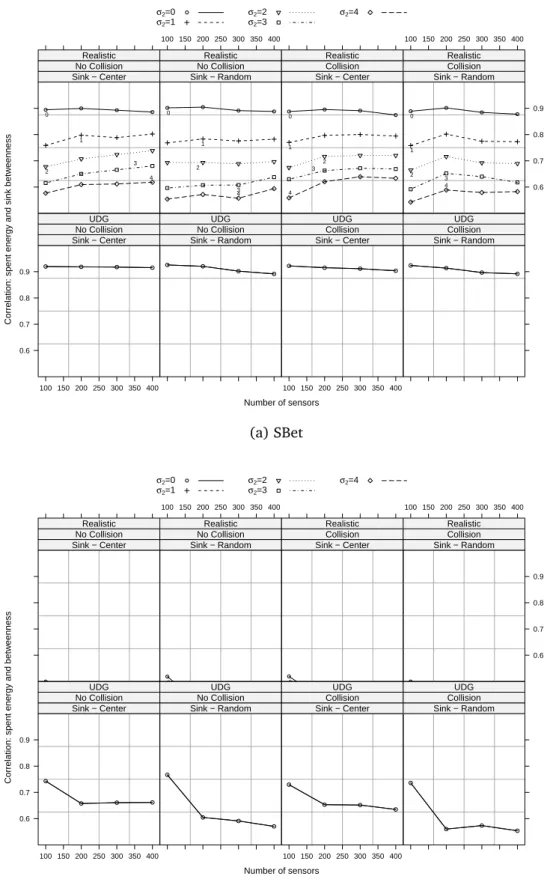
omit-ting the values of all other metrics, which did not appeared useful in our studies. Thus, we present the results of the correlation between the spent energy and two centrality metrics, namely Betweenness and SBet, when 4 situations are con-sidered: (i) simple gossip routing on URP deployment, (ii) simple random tree routing on URP deployment, (iii) simple gossip routing on Q-Model deployment, and (iv) simple random tree routing on Q-Model deployment. These situations were assessed for eight different scenarios, varying the channel model (UDG and Realistic), the collision model (no-collision and additive collision model) and the sink position (centered and randomly placed). We also vary the probability of the links becoming non-bidirectional (0< σ₂<4).

In all following situations the transmission is the task that employs most energy. Thus, we are looking forward to a metric able to indicate which node is more likely to transmit more packets.

✷✳✹✳✹✳✶ ❙✐♠♣❧❡ ❣♦ss✐♣ r♦✉t✐♥❣ ❛♥❞ ❯❘P ❞❡♣❧♦②♠❡♥t

mainly when the sink is randomly placed.

When we consider more realistic channels, SBet exhibits high correlation (consistently greater than 0.75) when σ₂ is zero (bidirectional channels) and 1 (realistic channels). It is clear that an increasing σ₂ degrades the correlation, due to packet loss. Notice that gossip routing herein considered employs routing level information that may not capture the real configuration in the presence of mostly non-bidirectional links, and may lead to additional packet loss and degraded correlation. Betweenness fails to capture which nodes are more likely to waste energy in realistic scenarios. Note also that in all situations of realistic scenarios the correlation is reduced to negligible values, which were discarded in Figure 2.5b to enhance the visualization.

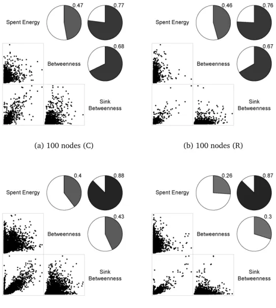
Figure 2.6 shows correlograms of selected scenarios, all with realistic wire-less channel models and collisions. The pies depicted above the diagonal illus-trate the correlation among the spent energy, Betweenness and Sink Between-ness, while the figures below the diagonal depict the scatterplots between these metrics. We observe that Sink Betweenness is almost independent of the number of nodes and of the sink position in more realistic models. When the number of nodes increases, the MAC looses the ability to manage collisions, and correlation degrades. In extreme situations, the delivery rate becomes quite low and the network metrics tends to degrade.

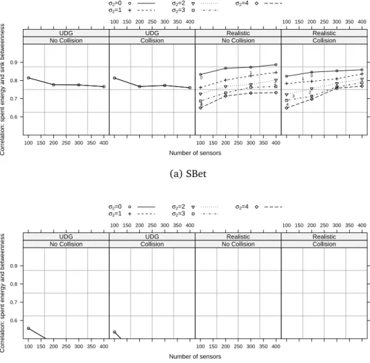
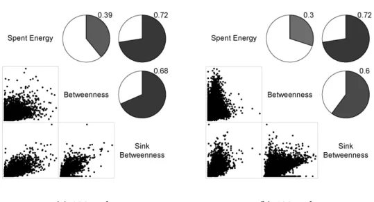
✷✳✹✳✹✳✷ ❙✐♠♣❧❡ r❛♥❞♦♠ tr❡❡ r♦✉t✐♥❣ ❛♥❞ ❯❘P ❞❡♣❧♦②♠❡♥t

Number of sensors

Correlation: spent energy and sink betw

eenness

0.6 0.7 0.8 0.9

100 150 200 250 300 350 400

Sink − Center No Collision

UDG

Sink − Random No Collision

UDG

100 150 200 250 300 350 400

Sink − Center Collision

UDG

Sink − Random Collision UDG 0 1 2 3 4 Sink − Center

No Collision Realistic

100 150 200 250 300 350 400

0 1 2

3 4 Sink − Random

No Collision Realistic 0 1 2 3 4

Sink − Center Collision Realistic

100 150 200 250 300 350 400

0.6 0.7 0.8 0.9 0 1 2 3 4 Sink − Random

Collision Realistic σ2=0

σ2=1

σ2=2 σ2=3

σ2=4

(a) SBet

Number of sensors

Correlation: spent energy and betw

eenness

0.6 0.7 0.8 0.9

100 150 200 250 300 350 400

Sink − Center No Collision

UDG

Sink − Random No Collision

UDG

100 150 200 250 300 350 400

Sink − Center Collision

UDG

Sink − Random Collision

UDG Sink − Center

No Collision Realistic

100 150 200 250 300 350 400

0

Sink − Random No Collision

Realistic

0

Sink − Center Collision Realistic

100 150 200 250 300 350 400

0.6 0.7 0.8 0.9

Sink − Random Collision Realistic σ2=0

σ2=1

σ2=2 σ2=3

σ2=4

(b) Betweenness

(a) 100 nodes (C) (b) 100 nodes (R)

(c) 400 nodes (C) (d) 400 nodes (R)

Number of sensors

Correlation: spent energy and sink betw

eenness

0.6 0.7 0.8 0.9

100 150 200 250 300 350 400

Sink − Center No Collision

UDG

Sink − Random No Collision

UDG

100 150 200 250 300 350 400

Sink − Center Collision

UDG

Sink − Random Collision UDG 0 1 2 3 4 Sink − Center

No Collision Realistic

100 150 200 250 300 350 400

0

1 2 3 4

Sink − Random No Collision Realistic 0 1 2 3 4 Sink − Center

Collision Realistic

100 150 200 250 300 350 400

0.6 0.7 0.8 0.9 0 1 2 3 4

Sink − Random Collision Realistic σ2=0

σ2=1

σ2=2 σ2=3

σ2=4

(a) SBet

Number of sensors

Correlation: spent energy and betw

eenness

0.6 0.7 0.8 0.9

100 150 200 250 300 350 400

Sink − Center No Collision

UDG

Sink − Random No Collision

UDG

100 150 200 250 300 350 400

Sink − Center Collision

UDG

Sink − Random Collision

UDG 0

1 2

Sink − Center No Collision

Realistic

100 150 200 250 300 350 400

0 1 2

Sink − Random No Collision

Realistic

0 1 2

Sink − Center Collision Realistic

100 150 200 250 300 350 400

0.6 0.7 0.8 0.9 0 1 2

Sink − Random Collision Realistic σ2=0

σ2=1

σ2=2 σ2=3

σ2=4

(b) Betweenness

(a) 100 nodes (C) (b) 100 nodes (R)

(c) 400 nodes (C) (d) 400 nodes (R)

Figure 2.8: Corrrelograms and scatterplots for tree routing and URP deployment, 100 and 400 nodes, centered (C) and randomly (R) placed sink