Agronomical effects of mechanical box pruning in cv. Merlot at central area of Spain

Master of Science in Viticulture & Enology

INSTITUT NATIONAL D

INSTITUTO SUPERIOR DE

AGRONOMICAL EFFECTS OF MECHANICAL BOX PRUNING

IN cv.MERLOT AT CENTRAL AREA OF SPAIN

supervisor 1:

Pilar Baeza

supervisor 2:

Carlos Lopes, Instituto Superior de Agronomía (ISA)

Jury:

President:

Jorge Manuel Rodrigues Ricardo da Silva (Phd), Full Professor, at Instituto

Superior de Agronomia, Universidade de Lisboa

Members: - Pilar Baeza (Phd), Professor at Universidad Politécnica de Madrid - Antonio Morata (Phd), Professor

- Ricardo Nuno da Fonseca Garcia Pereira Braga (Phd), Assistant Profe Instituto Superior de Agronomia, Universidade de Lisboa.

Master of Science in Viticulture & Enology

ATIONAL D'ETUDES SUPERIEURES AGRONOMIQUES DE MONTPELLIER AND

UPERIOR DE AGRONOMIA DA UNIVERSIDADE DE LISBOA

Master thesis

L EFFECTS OF MECHANICAL BOX PRUNING

IN cv.MERLOT AT CENTRAL AREA OF SPAIN

Miguel TEJERO PÁRAMO

2014-2016

Pilar Baeza, Universidad politécnica de Madrid

Carlos Lopes, Instituto Superior de Agronomía (ISA)

orge Manuel Rodrigues Ricardo da Silva (Phd), Full Professor, at Instituto

Superior de Agronomia, Universidade de Lisboa

Pilar Baeza (Phd), Professor at Universidad Politécnica de Madrid Antonio Morata (Phd), Professor at Universidad Politécnica de Madrid Ricardo Nuno da Fonseca Garcia Pereira Braga (Phd), Assistant Profe Instituto Superior de Agronomia, Universidade de Lisboa.

Lisbon, 2016

1

Master of Science in Viticulture & Enology

ONTPELLIER

ISBOA

L EFFECTS OF MECHANICAL BOX PRUNING

IN cv.MERLOT AT CENTRAL AREA OF SPAIN

rid (UPM)

Carlos Lopes, Instituto Superior de Agronomía (ISA)

orge Manuel Rodrigues Ricardo da Silva (Phd), Full Professor, at Instituto

Pilar Baeza (Phd), Professor at Universidad Politécnica de Madrid at Universidad Politécnica de Madrid Ricardo Nuno da Fonseca Garcia Pereira Braga (Phd), Assistant Professor, at

2

Acknowledgements

I have to express my gratitude to the “UPM” for welcoming me during the stage and to Pilar Baeza for supervising my thesis; sharing her valuable knowledge and guiding me during the whole process. Special mention also to “el Socorro state” team headed by Roberto for giving the chance to work in their fields and assisting us with materials and taking care of the vines so carefully.

I also would like to thank people from the laboratory Vanessa and Lucia same as the students of the national master of viticulture and enology UPM highlighting specially to Hector, Ana, Lili, Gabi; Manuel and Ivan whose amazing support and implication with the project in the field and laboratory was critical to take it to an end.

3

Abstract

Introduction: Global warming, economic crisis and globalization are the three pillars which

are altering the world in all the domains. In viticulture, a shortening of the grapevine phenology and an imbalance sugars/acidity derived from the new climatic conditions are forcing a reshuffle of the way of working in the field, in a more productive and sustainable with better quality. For that reason new pruning techniques have been developed in a way to adapt grapevines to the new conditions. Mechanical Box pruning has been proposed as promising alternative to implement in Mediterranean regions as a way to compensate the shortening of the phenology.

Material and methods: Trials have been carried out in central region of Spain, working with

irrigated vines of Vitis vinifera L. cv Merlot trained in vertical shoot positioning bilateral cordon system. Three pruning treatments were tested: T1 and T2 were traditional two-bud spur, and T3 Box pruning, with no lateral shoot or sucker removal in T2 and T3. Yield and ripeness parameters same as must phenolic composition (Glories method) were analyzed from early veraison until harvest.

Results and discussion: T3 vines showed higher yields compared to T2 and T1 reaching

28t/ha; 20t/ha and 12t/ha respectively. Higher canopy soil shade was also detected in T3 suggesting greater canopies and photosynthetic activity. Water efficiency was also higher in box pruning compared to manual pruning. No significant differences were detected at harvest concerning berry weight and must yield per berry. A delay in ripeness in T3 was clearly observed specially in TSS. Must composition showed differences at harvest in ph, TA and TSS between treatments being lower in T3 compared to manual pruning but all of them kept up in normal quality ranges. No differences were observed concerning phenolic composition, TPI or anthocyanins extractability.

Conclusions: Box pruned vines show a higher productive behavior in a more economic and

sustainable way with not big differences in terms of berry size or must quality, representing a valid alternative to produce higher yields with similar quality as the traditional spur pruning being well adapted to the new climatic and economic implications worldwide. Legislation should be adapted to new conditions and techniques making easier the implementation of new alternative methods.

Key words:

4

Table of Acronyms

- RDI= Regulated Deficit Irrigation - Ru= Ruggeri

- ETo=Evapotranspiration rate - RH%= Relative humidity - GDDºc= Growing degree days - Am= Aridity Index

- ETp= Potential Evapotranspiration - P= annual precipitation

- T= annual mean temperature - T ave= average temperature

- Tmax= average maximum temperature - Tmin= average minimum temperature - ᵠs= Stem water potential

- ET= Crop evapotranspiration - kc= crop coefficient

- Pe = effective precipitation

-Ce= efficiency of irrigation system (90%) - N= Nitrogen

- T1= Treatment 1 -T2= Treatment 2 -T3=Treatment 3

- p= significance value of probability

- LSD= Fisher’s least significance difference test

- SS= Shaded soil

- rpm= revolutions per minute - TSS= Total Soluble Solids -TA= Titratable acidity - TPI= Total Phenol Index - A280= Absorbancy at 280nm -A520= Absorbancy at 520nm - TAnt= Total Anthocyanins - EA= Extractable Anthocyanins - TH2= Tartaric acid

- HCl= Chloridric acid

- Adistilled= Absorbancy of the control sample

- A metha= Absorbancy of the sample mixed with Namethabisulphite - EXT%= Extractability

- Mp%= seed ripeness level - YAN= Yeast Assimilable Nitrogen - FAN= Free Assimilable Nitrogen - ns= not significant

- DOY= Day of the year

5

List of equations

(1): De Martonne aridity index (2): Crop evapotranspiration (3): Theorical irrigation needs (4): Must yield estimation (5): Shaded soil % estimation (6): shaded soil % estimation (7): Yield performance

(8): Titratable acidity determination (9): Total Phenol Index

(10): Etractable anthocyanins (11): Total anthocyanins (12): Extractability (13): Seed ripeness

6

Table of Contents

INTRODUCTION... 8

Outline ... 8

Viticulture and wine sector (Spanish approach) ... 10

Climatic implications ... 10

Economic implications ... 11

Alternative pruning systems ... 12

Aims ... 13

MATERIALS AND METHODS ... 13

Study placement ... 13

Vineyard characteristics ... 14

Climatic characterization ... 14

Stem water potential and irrigation needs ... 17

Nutrients requirements ... 19

Experimental treatments ... 20

Agronomical yield measurements ... 22

Berry weight ... 22

Shaded Soil (SS) ... 22

Harvest ... 24

Grape and must composition ... 25

Sampling method ... 25

Must extraction ... 25

Berry ripeness ... 25

Assimilable Nitrogen ... 29

RESULTS AND DISCUSSION ... 29

Agronomical responses ... 29

Must composition responses ... 35

CONCLUSIONS ... 41

REFERENCES ... 42

7

Index of tables and figures

Index of Figures

Figure 1: Grapevine climate Maturity groupings (Jones 2007) ... 9

Figure 2: Exports of Spanish wine in volume and value (MAGRAMA 2014 ... 11

Figure 3: Experimental Region map ... 14

Figure 4: Training system and autochthonous cover crop ... 14

Figure 5: Pressure chamber devise……… ... 17

Figure 6: Selected leaf for stemᵠ rolled in silver paper ... 17

Figure 7: Winter pruning shapes (3 treatments) ... 20

Figure 8: Box pruning system (source: Carbonneau and Cargnello 2003 ... 21

Figure 9: Experimental design scheme ... 22

Figure 10: Code panels ... 22

Figure 11: Shaded soil area example ... 23

Figure 12: Photoshop image edition ... 23

Figure 13: Shade amplitude determination ... 24

Figure 14: Harvest weight determination ... 24

Figure 15: Titratable acidity determination ... 26

Figure 16: Glories process ... 27

Figure 17: 100 berries weight evolution through berry development ... 31

Figure 18: Must yield /berry ... 31

Figure 19: Shaded soil % comparison ... 33

Figure 20: WUE comparison ... 34

Figure 21: TSS (ºbrix) evolution through berry ripening ... 36

Figure 22: pH evolution through berry ripening ... 36

Figure 23: Titratable acidity (g tartaric acid/L ) ... 37

Figure 24: Anthocyanins extractability and tannins content in seeds through berry ripening .. 40

Index of tables

Table 2: Average climatic conditions in the area (2010 –2015) ... 16

Table 3: Average climatic conditions during the experiment (2016) ... 16

Table 4: Irrigation needs for parcel 22 during the growing season of 2016 ... 19

Table 5: Technological ripeness parameters at harvest ... 32

Table 6: Shaded soil comparison ... 33

Table 7: Yield and WUE comparison ... 35

Table 8: Technological ripeness parameters at harvest ... 38

8

I.

INTRODUCTION

1. Outline

Climate change and grape price down trend registered in the last years (Santos et al 2012; MAGRAMA 2016), is forcing the wine industry to develop new alternatives permitting to enhance, in a new climatic context, productivity in order to satisfy the consumer’s demand without forgetting about quality; production costs and of course, environment preservation. Changes in the climatic conditions have been reported worldwide (Wolfe et al 2005; Jones 2007; Santos et al 2012; ICCP 2014) but the main differentiating aspects seem to be constant. In fact, an increase of the global surface temperature with a reduction in precipitation has been registered, having a critical effect on grapevine phenologic cycle (Jones 2007). Those changes have been related to a shortening of phonological phases; presenting earlier phenological events and a shortening of the cycles, altering qualitatively the balance in berry composition and flavours (Menzel et al 1999; Jones and Davis 2000; Jones 2007 Keller 2010). Up today, the climatic situation has had in general a beneficial effect on the fruit quality (Jones 2007). Nevertheless, ICCP last projections from 2014 determine the global surface warning for the end of the century in about 2ºC as an average taking into account all the possible scenarios. The relatively narrow climatic ranges where viticulture is developed and the future projections on global warming suggests, either an advantage, since new areas that were too cold for growing grapes would be able to do it for the first time and lowering additionally the risks of frost damage (Moonen et al 2002), or a potential drawback for the top current winegrowing areas. In fact, an increase of average temperatures and drought would shift the sugar ripeness earlier, obtaining higher sugar concentrations in the berry whereas the acidity drops unbalancing the final product. In addition, pressure on increasingly scarce water supplies, poses new issues to adequate the vines in areas where temperature and water are already limiting factors, turning challenging the production of quality grapes (Jones 2007, Melorose et al 2015).

Generally speaking, the optimal daytime temperature for grapevine growth, photosynthesis, yield formation, and fruit ripening is below 30ºC (Keller 2010) however, each grape variety has a specific average growing season temperatures range defining the climate-maturity ripening potential (Jones 2007; Figure 1). Then, impacts of climate change are not likely to be uniform across all varieties and regions, but are more likely to be related to climatic thresholds (Jones 2007). According to this information, it can be expected progressively changes in varieties grown, shifts in regional wine styles, and spatial changes in viable grape growing regions (Jones 2007).

9

Figure 1: The climate-maturity groupings given in this figure are based on relationships between phenological requirements and climate for high to premium quality wine production in the world's benchmark regions for each variety. The dashed line at the end of the bars indicates that some adjustments may occur as more data become available, but changes of more than +/- 0.2-0.6°C are highly unlikely. The figure and the research behind it are a work in progress (Jones, 2007).

To address, which is probably one of the most relevant challenges in viticulture for the next decades, several trials have been already carried out along the world. Cultural practices can at best be used to fine-tune what nature imposes in any given season(Keller 2010). Most of the research about this subject is focusing on new agricultural practices permitting in one hand to increase yields on quality fruit, in a more sustainable and economical way, and in the other hand, to delay sugar ripeness taking into account the self regulation capacity of the plant in a way to compensate the early phenology induced by the new climatic conditions. Among those techniques, regulation of the crop load of the plant through alternative pruning systems is probably one of the most promising solutions. The biggest the adaptation capacity is, the

10 lowest the vulnerability and the biggest the capacity of reducing negative effects coming from the climate change and to face market risks (Sanchez et al 2014).

2. Viticulture and wine sector: Spanish approach

Grapevines are planted in every region of Spain, inland and island, being more concentrated in the central area, northern and southern plateau. The richness in grape varieties combined with the complex topography, with important amplitude of altitudes; high diversity of locations; exposures and climates, allow having a great variability in planting areas enabling the production of a large spectrum of wines (CYTED 2012).

Generally speaking, spanish central areas are characterized by having long summers with high insolation and temperatures permitting a correct ripening even in late varieties. In addition, rain events are limited and irregularly distributed along the season, being almost absent during the growing season increasing water deficit. Spring frosts are also present particularly in high areas (CYTED 2012). However, climate change factors are susceptible to significantly affect viticulture in Spain, some of them are described in table 1.

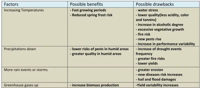
Table 1. Potential effects of climate change in spain

Factors Possible benefits Possible drawbacks

Increasing Temperatures - Fast growing periods - Reduced spring frost risk

- water stress

- lower quality(less acidity, color and tannins)

- Increase in alcoholic degree - excessive vegetative growth - fire risk

- new pests rise

- Increase in performance variability Precipitations down - lower risks of pests in humid areas

- greater quality in humid areas

- increase of drought events frequency

- greater fire risks - lower yields

More rain events or storms - greater erosion

- new diseases risk increases - hail and flood damages Greenhouse gases up - increase biomass production -Yield variability increases

11

b) Economic implications

Despite the strong decrease in planted area in European countries, Spain, with about 1.037 kha of vineyards, remains as the country with the biggest area under vines in the world followed by China and France, accounting 14% of the global area under vines (OIV 2015). However, it cannot be stated the same for grape and wine production. According to the OIV report 2015, Spain produced 15% of the total wine in the world in 2014. 38,6 Million hl of wine was produced as an average from 2008 till 2013 and between 5300 – 7700 Tons of grapes from 2010 to 2013 equally distributed between red and white grapes, registering big variations between vintages( MAGRAMA 2014). In Spain, 85% of the area under vines is potentially suitable to produce quality DOP wines.

Spanish Wine consumption is relatively low compared to other big wine producers; in addition, international competition is intensifying due to the globalization and the economic crisis worldwide. Thus, Spanish wine is mainly focused in export (Sanchez et al 2014). Spain is along with New Zealand and Australia is considered a “net exporting country “where consumption over production ratio is highly above than 100% (OIV 2015).With 22,6Mhl of wine exported in 2014 accounting 22% of the total wine exports, Spain is at the top of the global wine trade flow, specially oriented to other members of the U.E. However, with an average price around 1€ per Litter of wine which is less than a half of the global average price, defines clearly Spanish wine exportation as oriented to more economic and affordable product (Salgado 2014).

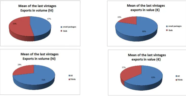
It is undeniable that, low value bulk wine is a critical part of the Spanish wine market and one of the main products to be exported specially to France (Sanchez et al 2014 )(figure 2).

Figure 2: Exports of Spanish wine in volume and value (MAGRAMA 2014: data taken from 2008-2013)

12 This exportation trend of big volumes of wine may offer an interesting chance to develop new agronomical alternatives permitting not only to increase the final production with and increase in value, but also lowering significantly production and labor costs.

3. Alternative pruning systems

According to Professor Winkler from Davis University California, pruning comprised the removal of the living vegetative parts of the plant such as canes, leaves or shoots and was responsible maintaining the shape of the canopy, yield regulation, and grape quality (Winkler et al 1974). From the beginning of the viticulture, several pruning systems have been developed according to the country; region; and grape variety (De Toda et al 1999), but the basis of the traditional manual pruning remained the same until our days, removing at least 85% of the annual growth of the plant (Winkler et al 1974). Traditional manual pruning still represents an excessive labor costs for the vine growers and time consuming (De Toda 1999). Those effects were even more severe for extensive producers being more profitable to switch to mechanization of the pruning, increasing yields and reducing considerably labor costs and time, saving in some cases more than 40 % (Rieger 2011;Reynier 2012 ). But, in detriment, sugar accumulation inside the berries was reduced, affecting to the final quality of the product (Reynolds and Wardle 1993, Morris and Cawthon 1981, Freeman and Cullis 1981).

New pruning systems, suitable with mechanization have been studied during the last decades in order to solve the above mentioned problem. Techniques like minimal pruning or box-hedge pruning have got some promising results with classical grape varieties in determined warm areas of the new world like Australia (Clingeleffer1984;2013,Sommer 1994; Possighan 1995). However, contradictory results have been registered in long term studies in European countries so far (Schultz et al 2000; Schultz and Weyand 2005; deToda 1999; Lopes et al 2000). Concerning mechanical Box pruning, it has been shown in previous studies to induce the production of smaller clusters with reduced weight but in greater number per vine, due to the self regulation capacity of the plant facing a higher crop load (Lopes et al 2000). As a consequence, significantly higher yields per vine with no significant changes or light improvements in the quality of the wines or musts have been observed (Lopes et al 2000, Smithyman et al 1997;Cruz et al 2010; Rieger 2011) allowing a better use of the “terroir” potential. Despite the increase in shoot number per vine, reduced vigour has been registered in terms of pruning weight, having potential longevity issues in long term practices (Lopes 2000; Cruz et al 2010). Shoot thinning and a Regulated deficit of irrigation (RDI) have shown beneficial effects in berry composition and wine quality (Robinson and Smart 1991, Lopes et al 2000). However, overcrop risk; diseases susceptibility and reduced plant longevity are still issues for those systems affecting drastically to the final quality (Morris and Cawthon1981, Smithyman et al 1997). Then, higher levels of understanding and management skills are required. Alternate box pruning and normal manual pruning along the years may be an alternative to mitigate the disadvantage of vigor reduction and promoting higher plant longevity (Lopes et al 2000).

13

4. Aims

The general objective is to determine the agronomical effects of viticultural practice based on simulated mechanical box pruning for a possible integration as a new vine growing method, checking the adaptability to the future conditions in Mediterranean regions under drip irrigation.

The particular objectives are:

1. To compare the agronomic performance of Merlot/140Ru traditionally pruned versus box pruning training system by using yield and vigour parameters, checking possible delays in berry development.

2. To compare the basic must composition of Merlot/140Ru traditionally grown versus box pruning. An increased production without a minimum quality would trigger a devaluation of the product, then monitoring the main quality parameters in must composition were carried out periodically to check the acceptability of the product according to the standards.

3. To compare phenolic ripeness and technological ripeness of both growing systems as a way to check if effectively a delay in berry ripeness is happening or not.

4. To evaluate the water efficiency in both growing systems to compare the sustainability of the treatments.

II.

MATERIALS AND METHODS

1. Study placement

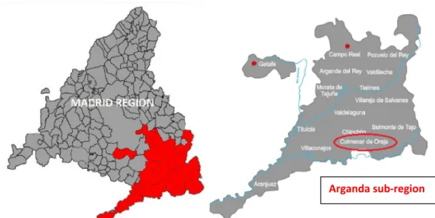
The experiment was conducted at the ‘‘El Socorro’’ Experimental Vine growing Centre belonging to the “Instituto Madrileño de Investigación y Desarrollo Rural y Agroalimentario (IMIDRA)”, located in the southeast of the Madrid region, Spain (latitude40° 8'10.17"N, longitude 3°22'35.41"O) (Figure 3).

The original soil at the site was composed by loam and limestone classified as Calcixerollic Xerochrept which is described as coarse-loamy, carbonated and thermic soil with low Organic matter content. The drainage capacity of the soil was good and coarse elements and the surface salinity were negligible. The rock content was in class 3 and the slope smaller than 2% (Linares Torres, 2009)

The climate in the region is mild-continental Mediterranean with hot and dry summers and cold winters. The average rain recorded was 460mm per year.

14

Figure 3: experimental region (taken from “consejo regulador D.O Vinos de Madrid”)

2. Vineyard characteristics

The trial was carried out in 1 ha Merlot vineyard trained in Sprawl bilateral cordon Royat with orientation North-South and a trunk height at 0,8m.The vineyard was originally planted 2000 with Merlot (clone 346) onto 140 Ruggeri with dimensions of 2.2 x 1.5 m(Figure 4). Natural cover crop made by autochthonous grass grows in between the rows.

Figure 4: bilateral cordon royat training system and autochthonous cover crop

3. Climatic characterization

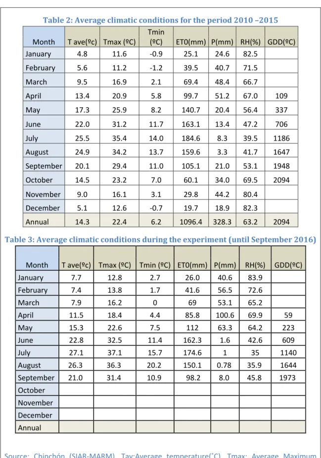
According to table 2, between 2010 and 2015, the area was characterized by warm and dry summers and cold winters. In fact, annual average temperatures were higher than 14ºC

15 (overpassing easily 35ºC Tmax in summer) and average precipitations for the whole year were lower than 400mm, mainly along early spring and fall. Plants were submitted to a regulated water deficit during summer depending exclusively on irrigation water during the hottest months, July and August. This could also be noticed by the low RH% and a great evapotranspiration rate (ETO) during this period, been necessary a regulated supplement of irrigation periodically. Negative temperatures registered in March suggested also the risk of spring frost damages for early phenology varieties in the region.

Taking into account the growing degree days (GDDºC) during the growing season from the 1st of April until the 31st October (Northern hemisphere), we obtained 2094ºC as an average of the 6 years. According to Winkler index, the climatic profile of this area would fit with a Region IV (values between 1945-2222ºC) described as a region suitable to produce qualitative fortified and sweet wines or raisins (Amerine and Winkler 1944).

De Martonne (1926) proposed his aridity index (Am) as an alternative for local scale using temperature as a proxy for Potential evapotranspiration (ETp) as follows:

(1) Am= _{( )}

(where, P (mm) is the annual precipitation and T (ºC) the annual mean temperature The equation is appropriate for temperatures greater than –9.9C).

De Martonne aridity index decreases (approaches zero) with increasing aridity. Using the data from the table x we obtain a Am of 13,5 corresponding with an Arid-Steppic zone (range 15-5). As a contrast, climatic conditions of the study year were slightly different compared to the previous years. According to the climatic data collected in the area (Table 3), 2016 was described as a year with warm winter, however the temperatures were sufficiently low to assure a correct plant dormancy. A fresh and particularly humid spring, specially during April and May when intense rain events happened in the area, and a hot and dry summer. Nevertheless, cumulative degree days were similar at harvest time permitting, even if 2016 was not a “Typical” year comparing to the previous ones to be considered as a representative year for the study.

16

Table 2: Average climatic conditions for the period 2010 –2015

Month T ave(ºc) Tmax (ºC)

Tmin (ºC) ET0(mm) P(mm) RH(%) GDD(ºC) January 4.8 11.6 -0.9 25.1 24.6 82.5 February 5.6 11.2 -1.2 39.5 40.7 71.5 March 9.5 16.9 2.1 69.4 48.4 66.7 April 13.4 20.9 5.8 99.7 51.2 67.0 109 May 17.3 25.9 8.2 140.7 20.4 56.4 337 June 22.0 31.2 11.7 163.1 13.4 47.2 706 July 25.5 35.4 14.0 184.6 8.3 39.5 1186 August 24.9 34.2 13.7 159.6 3.3 41.7 1647 September 20.1 29.4 11.0 105.1 21.0 53.1 1948 October 14.5 23.2 7.0 60.1 34.0 69.5 2094 November 9.0 16.1 3.1 29.8 44.2 80.4 December 5.1 12.6 -0.7 19.7 18.9 82.3 Annual 14.3 22.4 6.2 1096.4 328.3 63.2 2094

Table 3: Average climatic conditions during the experiment (until September 2016)

Month T ave(ºc) Tmax (ºC) Tmin (ºC) ET0(mm) P(mm) RH(%) GDD(ºC)

January 7.7 12.8 2.7 26.0 40.6 83.9 February 7.4 13.8 1.7 41.6 56.5 72.6 March 7.9 16.2 0 69 53.1 65.2 April 11.5 18.4 4.4 85.8 100.6 69.9 59 May 15.3 22.6 7.5 112 63.3 64.2 223 June 22.8 32.5 11.4 162.3 1.6 42.6 609 July 27.1 37.1 15.7 174.6 1 35 1140 August 26.3 36.3 20.2 150.1 0.78 35.9 1644 September 21.0 31.4 10.9 98.2 8.0 45.8 1973 October November December Annual

Source: Chinchón (SIAR-MARM). Tav:Average temperature(˚C). Tmax: Average Maximum temperature (˚C). Tmin: Average Minimum temperature (˚C). ET0: Monthly evapotranspiration (mm). P: Precipitation (mm).RH: Average relative humidity (%). GDDs: Accumulating Growing Degree Days (˚C, 10˚C based); Daily data in Annex 1)

17

4. Stem water potential and Irrigation needs

To assure an equal water availability level for each treatment, regulated drip irrigation supplement was necessary. To assess the right amount of water required for each treatment and at which time some previous measurements were necessary to be taken.

Daily Ψs was defined as the result of whole plant transpiration, and soil and root/soil hydraulic conductivity indicating in one hand the capacity of grapevine to conduct water from the soil to the atmosphere representing a good plant water status indicator (Choné et al 2001; Begg and Turner 1970). Ψs was measured on a nontranspiring leaves being bagged previously with aluminum foil at least 1 hour before the measurements (Figure 6) preventing leaf transpiration and equaling leaf potential to Ψs (Choné et al 2001; Begg and Turner 1970). Leaves were selected every week from the same vineyard spots distributed among the 3 treatments, paying special attention to select leaves from the shaded side of the row for bagging as a way to avoid possible overheating during bagging period (Choné et al 2001).

Irrigation period started once vegetative growth stopped. Irrigation management was carried out carefully according to the respective Stem water potential (Ψs) in each treatment block which was measured once a week in a specific day (before the new irrigation period of the following week) at 13:00 with the pressure chamber PSM 600D (figure 5). The aim was to irrigate to keep Ψs of -1,1 MPa, inducing moderate water stress level on the vine (Baeza et al .2007). Irrigation was split into two or three days per week depending on the dose.

Figures 5 and 6: Pressure chamber devise for ᵠs determination (left) and selected leaf rolled in silver paper inducing stomata closure (right)

To determine the irrigation needs, climatic conditions of the previous week and the water consumption of the vineyard were taken into account in the following calculations.

18 In order to calculate the amount of hours to irrigate, the following calculations were

developed

(2) ET = Kc×ETo ET: The crop Evapotranspiration.

Kc: % of the ETo (Kc = 0.3 was the coefficient throughout all the applications, based on previous trials done at “El Socorro”, leaf area index developed and weather forecast (Williams y Ayars, 2005); from the second week of august until harvest Kc became 0,45due to the extreme draught conditions).

ETo: The reference evapotranspiration (for the calculation of the ETo of the previous week was used).

Therefore the irrigation need in mm is calculated subtracting the effective precipitation (Pe) of the previous week from the crop evapotranspiration (ETo) and this divided by the efficiency of the irrigation system (Ce).

(3) Theoretical irrigation need (mm) = × − (Pe) Pe: Effective precipitation.

Ce: Efficiency of the irrigation system (90%).

Drip irrigation system was installed with 2 drips per plant and the irrigation flow is 2.3 L/hour. This means 4.6 L/hour/plant and 1.39 L/m2 (with planting dimensions 2.2 x 1.5) and 1.39 mm/hour (Botha 2013). Results were shown in Table 4.

19

Table 4: Irrigation needs for parcel 22 during the growing season of 2016

5. Nitrogen requirements; fertilization and phytosanitary

treatments

Treatments were fertilized separately to supply equally the Nitrogen according to the vigour, then 20 N Units/ha for treatment 1 and 30 N units/ha treatments 2 and 3 were supplied. NO₃NH₄ at 34% richness diluted in cold water 5ºC was selected compound applied with irrigation weekly from the 15Th April (budburst) until 1st July (green berries stage), 11 weeks in total. Phytosanitary treatments against the main pests and fungal diseases in the region were applied equally in all the pruning treatments.

Week Treatment 1 hours Treatment 2 hours Treatment 3 hours 20-26 June 0 0 0 27 June-3 July 4 4 4 4-10 July 0 0 4 11-17 July 10 10 10 18-24 July 10 10 10 25-31 July 8 13 13 1-7 August 10 10 15 8-14 August 10 10 15 15-21 August 10 10 17 22-28 August 5 10 10 29 August-4 Sept 5 10 10 5-11 Sept 12 17 17 12-18 Sept 15 15 15 19-25 Sept 10 10 15 26 Sept-30 Oct 10 10 10

Total irrigation hours 119 139 165

20

6. Experimental Treatments

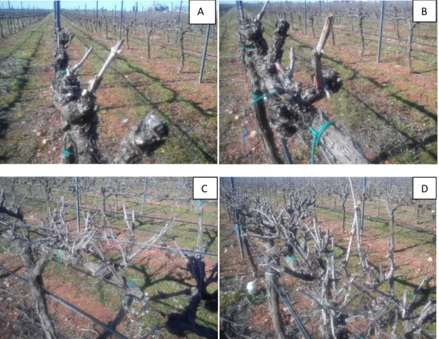
 Treatment 1 (control test) = traditional spur pruning leaving 2 buds per spur and in general around 14 buds per vine to reach 10 shoots per row meter (picture A). Green practices were performed the 6th _{June including shoot removal of secondary shoots} and suckers in cordon and cleaning of trunk, leaving only the chosen amount of shoots.

 Treatment 2 = spur pruning leaving 2 buds per spur and in general around 14 buds per vine. No shoot removal; leaving the laterals and suckers to develop, but the trunk was cleaned of suckers (picture B).

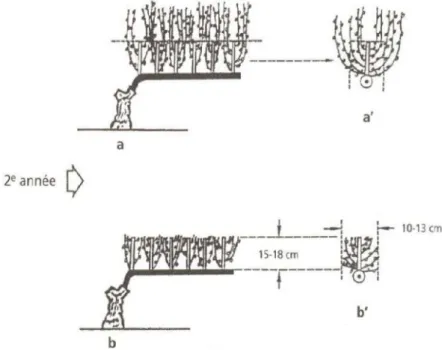
 Treatment 3 = simulated mechanical box or hedge pruning system keeping about 3 buds per spur and in general around 21 buds per vine. No shoot removal; leaving the laterals and suckers to develop but the trunk was cleaned of suckers (pictures C and D). This method consists in a non selective uniform pruning resulting in a box shape of the canopy as described in the Figure 8, later on, the canopy conduction was established in sprawl.

Figure 7: A= treatment 1(spur pruning 14 buds per vine to reach 10 shoots per row); B= treatment 2(spur pruning 14 buds per vine to reach 10 shoots per row and no shoot removal);

B A

D C

21

C and D= treatment 3 box pruning (3 buds per spur and in general around 21 buds per vine and no shoot removal)

Pruning was carried out for all the treatments between end of February and mid March.

Figure 8: Box pruning system, unselective pruning keeping box shape canopy, cutting 15cm far from the cordon (source: Carbonneau and Cargnello 2003)

The experiment was structured in a stripped-block design with the three treatments, replicated 3 times. Each replication was divided into 3 blocks with 30 vines (Figure 9). Treatments; repetitions and blocks were encoded in a 3 digit code (Figure 10) from 1 to 3 being the first number related to the treatment applied; the second representing the repetition number and the last one the selected block. According to this, code 111 refers to treatment 1 (manual spur pruning), repetition 1 and block 1. Extra boundary rows were planted with cv. Malvasia grape (in the margins of the vineyard) and with Merlot (in between the control rows) as a protective layer to avoid any interaction between treatments or the margins of the vineyard.

22

Figures 9 and 10: experiment design scheme (left) representing 3 different pruning treatments with 3 replications and rows divisions in subparcels, 27 in total , each one codified in the field using a 3 digit code in yellow panels(right).

All the results were processed by a Statistics software (STATISTIX), applying analysis of variance (ANOVA) type III sum of squares in a multifactorial design, revealing possible interactions between the treatments and the blocks. Analysis was performed separately for factors which interaction seemed to be clear, showing a significance value of probability (p)≤0,05. Significant differences between averages was tested applying a Fisher’s least significant difference method (LSD) with a 5% risk to consider each pair of means significantly different even when the real difference was 0.

7. Agronomical yield measurements

a. Berry Weight and Must Yield per berry

100-berries per single block were collected weekly from pea size till harvest to track berry ripening then, stored in a refrigerator with dry ice for further analysis in the laboratory. Samples were packed in small plastic boxes coded as the respective blocks with a known weight. In the laboratory each sampling box was weighted previous balance calibration subtracting later the weight of the plastic box itself to get the sample weight.

To estimate must yield per berry, the following calculation was developed:

(4)

must yield

=

º ( )

b. Shaded Soil (SS)

To obtain balanced vines in terms of vegetative growth and reproductive organs, a correct optimization of vineyard management is crucial. For this purpose, monitoring of canopy vigour

23 is an important tool (Fuentes et al 2014). In this study, Shade Soil was measured as an accurate way to estimate canopy size and vigour.

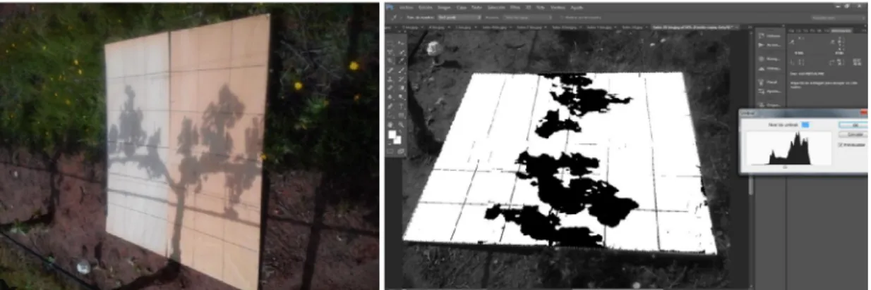
The same 10 vines were selected for periodic measurements. For each vine a flat board (1,2m x 1,2m) was placed just beneath the canopy as a screen to project the canopy shade, then photos of the whole device were taken using a digital camera (Figure 11). The board was marked with a grid that would be used later to determine the real surface of the shade. The pictures were taken around 11:00 am, profiting of the optimal sun angle of the sunlight taking into account the orientation North/South of the vineyards, permitting a clear projection of the shade on the board (Williams and Ayards, 2005).

All the photos were processed and treated with “Adobe Photoshop CS6” software, removing possible artifacts that could spoil the results and applying filters to change the image to black and white (Figure 12). This previous treatment permits the software to calculate the percentages of black and white surfaces which could be translated to percentage of shaded surface per plant, since the surface of the board is known (Botha 2013).

Figure 11(left): projection of the canopy shade on a wood board (shaded soil area example picture) .Figure 12(right): Photoshop image edition applying different filters to estimate shaded area

Calculation:

Plantation density= 3,3m2/plant

(5) SS(%) =

( / )

×

Starting from the 21 of June, canopy shade turned bigger than the flat board making impossible the measurement of the shaded soil with accuracy. As a consequence, the measurement methodology was switched to canopy shade amplitude determination. Measures were taken in the same spots as the pictures, taking 10 measures from trunk to trunk with 15 cm gap and paying special attention to the canopy porosity which was subtracted from the total shade amplitude (Figure 13). In this case shaded surface % was determined as follows:

(6) SS(%) =

24

Figure 13: Shade amplitude determination using a measuring tape each 15 cm from trunk to trunk, taking into account porosity.

c. Harvest

A determined number of plants per sub block were selected to be harvested manually in 25kg harvest boxes. All the harvested clusters were counted and weighted as shown in the Figure 14permitting the estimation of yield performance per ha for each treatment. Based on the parameters described in the section bellow “Berry maturity” the date of harvest was defined rigorously for each treatment. 24ºBrix with TA around 5 g/L and pH close to 3,5 where the main criteria for harvest decision making, resulting treatment 1 as the first to be harvested (5th of September) followed by treatment 2 (13th of September) and finally treatment 3 (20th,27thof September and 3rd,4th October respectively)

Calculations: crop performance was calculated as follows

(7)

=

º

x

Figure 14: Harvest weight using 25kg harvest boxes on a digital weighing

25

8. Grape and must composition

a) Sampling Method

Berry samples were collected weekly until harvest using plastic boxes or plastic bags in the case of the Glories method marked with the 3 digit code with the treatment; replication and block numbers. Later, all the samples were stored in a refrigerator and carried to the laboratory to be processed.

In order to get a more statistically representative sampling and a lower error, samples were taken randomly, picking berries from all parts of the cluster (tips, middle and shoulders) paying attention to collect only one berry per bunch and from both sides of the row in equal parts. For each of the 27 blocks, 100 berries sample was dedicated to technological maturity analysis and another 250 berries sample for phenolic maturity (Botha 2013).

b) Must extraction

All the samples were submitted separately to a manual rotating sieve in order to extract the liquid phase, separating the seeds; skins and pulps from the must. Low pressures were applied to avoid possible release of greenish particles from the seeds to the must.

Later on, the liquid was filtered and moved into small tubes to be centrifuged at 3000 rpm during 5 minutes to assure the separation of the remaining solid particles present in the must. Then clear liquid was collected in 50 mL recipients for further analysis.

c) Berry maturity

A fruit with the optimal ripeness level is the base of a good quality must or wine. For that reason the right determination of harvest date is critical. A common practice to select the harvest date and control of the berry ripeness is by monitoring the evolution of the different compounds in the grapes from veraison (Reynier 2012). In this experiment, different parameters of technological and phenolic maturation have been registered as complementary methods of berry ripeness determination.

Technological ripeness parameters

This section is based on the variability on berry weight and content in sugars and acids along berry ripening until harvest.

Berry Weight:

As explained above samples were weighted one by one in the laboratory using a digital balance taking note of the weight of 100 berries and the average weight for a single berry (dividing the measure by 100). The balance was previously calibrated and zeroed using an empty sampling bag.

26 Total Soluble Solids (TSS):

A few drops of the liquid samples were tested using an Atago® Pallete-Series PR-32 refractometer previous calibration with distilled water, rising with fresh distilled water and paper in between measurements. Results were expressed in ºBrix. The device turned directly the data at 20ºC.

pH:

Measurements were carried out using a Crison® MicropH 2001 pHmeter with a glass electrode; previous calibration using supplied buffer solutions at 20ºC. To read the pH of the sample, the probe was dept into the must.

Titratable Acidity (TA):

1,0 mL sample from the clear liquid was transferred to a new recipient and filled with distilled water up to 50 mL of volume. To determine the TA, samples were submitted to titration with NaOH until an end point of 8,2 at 20ºC, (Ough and Amerine 1988) Measurements were taken with an automatic pHmeter Metrohm®Titrino 702SM provided with 824 Easy sample Changer rotating tray (Figure 15). Results were given by the following formula expressed in grams of tartaric acid per liter:

(8)

= 3,75 × V

Phenolic ripeness parameters

This section is focused on the variability on the main phenolic compounds present in the berry, anthocyanins and tannins at harvest. Reynier 2012 describes phenolic ripeness as the capacity of the berry to release those phenolic compounds to the must.

Total Phenol Index (TPI):

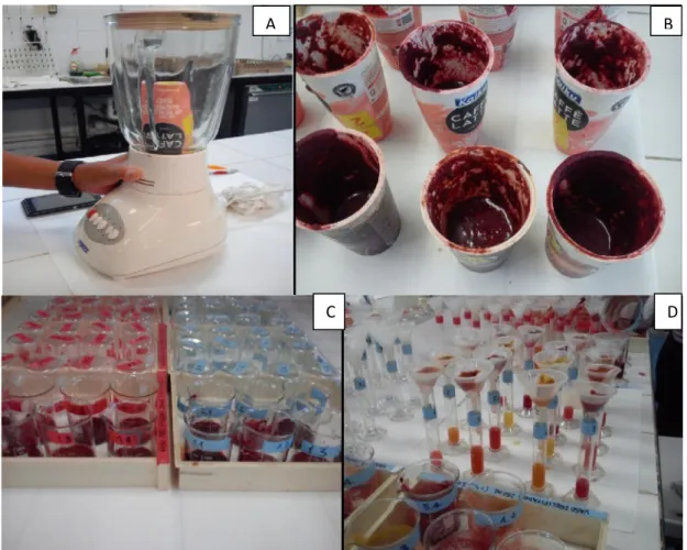
The methodology usedin this experiment was described by Glories and Augustin (1993) for polyphenol analysis (Figure 16).After crushing mechanically the berries, and having measured the ºBrix for each sample, 50mL of liquid were collected. Then 50 mL of tartaric acid solution at pH 3,4 was added to each sample, keeping them macerating for 4 hours previous to the filtration with a fiberglass filter. 1 mL of the filtrated liquid was taken apart and diluted 1/41

Figure 15: TA determination using an automatic titration machine for multiple samples

27 with distilled water to be analyzed with a Spectrophotometer zeroed also with distilled water. Absorbancy was read at 280nm (A280) and converted to TPI through the following formula:

(9)TPI =A280 × Dilution factor

Figure 16: Glories process (A and B: Mechanical crushing of the samples; C: maceration with 2 different acids, HCl( Red label) and Tartaric acid(Blue label);D: filtration using fiberglass)

Total and Extractable Anthocyanins:

Another aspect of the Glories method is the determination of both total (TAnt) and extractable anthocyanins (EA) using again spectrophotometry. Samples used for extractable anthocyanins were submitted to a 4 hours maceration in a tartaric solution at pH 3,2 (TH2), meanwhile the samples designated to total anthocyanins analysis were macerated in a hydrochloric acid solution (HCl) at pH 1. After completing the maceration, liquid phase was separated, extracting 1 mL from each sample and mixing it with 1 mL Ethanol 0.1% HCl and 20 mL HCl 2%. Finally, 10mL from each sample were blended with 4 mL of distilled water whereas another 10mL were mixed with 4mL of Sodium metabisulphite 15%, which reacts with the anthocyanins of the solution forming uncolored compounds (Berké et al 1998). A spectrophotometer was used to measure the Absorbancy at 520nm wavelength (Adistilled and Ameta). In the case of the second blend, samples were submitted to 20 minutes maceration previous to the analysis. Results were translated to mg of Malvidin per litre using the following formula:

A B

28 (10)Extractable anthocyanins (mg/L)= (Adistilled TH2- Ameta TH2) x 2 x 875

(11)Total anthocyanins (mg/L)= (Adistilled HCL- Ameta HCL) x 2 x 875 (Extinction Coefficient of Malvidin= 875)

Anthocyanins Extractability (Ext%)

Extractability is based on the comparison of the anthocyanin concentration of two different solutions obtained after macerating the grapes for four hours at two different pH values (Romero et al 2005). EA% was determined indirectly using the results provided by Glories method through this the following formula:

( ) % =( − )

The lowest Ext%, the highest anthocyanins extractability is. Standard values ranges from 20 to 70 % increasing with berry maturity (Glories 2001)

Seed ripeness (Mp%)

Seeds are the biggest reservoir of condensed tannins in the berry, assembled in the vacuoles of the seed coat in small subunits and, to a much lesser extent, the skin cells of the berries cultivars and rachis (Amrani and Joutei 1994; Souquet et al 1996; Thorugate and Singleton 1994, Keller 2010).

It has been shown that, when high levels of this compounds coming from the seeds are released to the must after a maceration process with the seeds, induce negative effects in the sensory perception of the final product particularly associate to excessive astringency or green flavours due to the presence of sharp green tannins in the wine (Glories 2001). This parameter decreases with berry maturity, for this reason optimal berry seed ripeness is fundamental to avoid possible sensorial defects.

Mp% represents the contribution of tannins released from the seeds that contributes to the global phenolic content of the extract. Standard values ranges from 0 to 60 % being higher when the tannins from the seeds are easier releasable to the must, (Glories 2001)

(13) Mp%=

, ×

×

29

d)

Yeast Assimilable Nitrogen (YAN)

Nitrogen plays a major role in many of the biological functions and processes of both grapevine and fermentative microorganisms. In fact, fermentation kinetics and formation of flavour-active metabolites are indeed affected by the nitrogen status of the must, (Bell and Henshckel 2005). To assure a complete fermentation of the must, yeast requires certain amount of nutrients based on Nitrogen. Nevertheless, not all the Nitrogen forms are available for the yeasts, only FAN (Free Amino Nitrogen) or ammonia NH4+ are consider as YAN. In the literature, it has been defined a threshold of 150 mg N/L of yeast-assimilable nitrogen to complete alcoholic fermentation (Keller 2010).

Sorensen method was the selected practice to determine the FAN in the must. This method is based on formaldehyde (40%) titration brought to pH 8.0 and has shown a high degree of sensitivity being reliably used as a routine procedure for the determination of assimilable nitrogen in wine industry (Ribeiro and Faia 2007).

Having crushed and centrifuged every grape sample. 50 mL of clear must was separated from each sample and basified up to pH 8 by adding NaOH 1M. Later, 20mL of Formaldehyde was added reacting with the FAN compounds of the sample and increasing the acidity of the solution. Final solutions were titrated back to pH 8 with NaOH 0,1 M taking note of the volume added to be used for the following calculations:

(14) FAN (mg/L)= (mL NaOH 1M) x 56

III.

RESULTS AND DISCUSSION

1. Agronomic responses

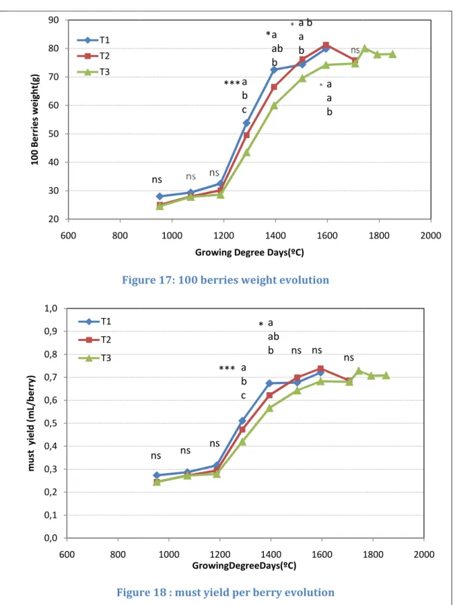
Results extracted from the monitorization of the berry development from berry set until veraison show a progressive increase in terms of berry weight in all the treatments as expected, reaching approximately the maximum weight at the end of the lag phase as described by Keller 2010 (Figure 17). Significant differences between treatments were shown during berry growth, differing specifically T3 from the others. In fact a short delay was noticed in the case of treatment 3 during berry growth period, reaching the maximum berry weight slightly later compared with the other 2 treatments. No significant differences seem to appear at the end of the berry growth suggesting that at the end all the treatments reach similar berry weight, in contrast with the results described in the literature where the berry weight was significantly lower in box and minimal pruning systems compared to manual system (Freeman and Cullis 1981; Reynolds et al 1993 Smithyman et al 1997; Striegler et al 2000). This observation was probably due to the fact that all the treatments were irrigated to optimal conditions according to the canopy management applied.

30 Similar trend was also observable in must production rates per berry (Figure 18), having highly significant differences between treatments at the beginning of berry growth the lag phase. Same delay was observed in T3 compared to the other treatments in the same period. However, once again, the differences between treatments in must production per berry were not significant at the end of berry development.

Figure 17: 100 berries weight evolution

Figure 18 : must yield per berry evolution T1= treatment 1(spur pruning

2(spur pruning 14 buds per vine to reach 10 shoots per row

treatment 3 box pruning (3 buds per spur and in general around 21 buds per vine and no shoot removal). ns=not significant ;*,**and*** represent significance at P=0,05,0,01 and 0,001 levels respectively; Figures for differ

significantly at p≤0.05). 20 30 40 50 60 70 80 90 600 800 100 Ber ries weight(g) T1 T2 T3 0,0 0,1 0,2 0,3 0,4 0,5 0,6 0,7 0,8 0,9 1,0 600 800 must yield ( mL/b err y) T1 T2 T3

Figure 17: 100 berries weight evolution

Figure 18 : must yield per berry evolution (spur pruning 14 buds per vine to reach 10 shoots per row

14 buds per vine to reach 10 shoots per row and no shoot removal) 3 buds per spur and in general around 21 buds per vine and no shoot significant ;*,**and*** represent significance at P=0,05,0,01 and 0,001 levels Figures for different treatments, followed by the same letter, do not differ

1000 1200 1400 1600

Growing Degree Days(ºC) ns a b c a ab b a b a b a a b * *** 1000 1200 1400 1600 1800 GrowingDegreeDays(ºC) ns a ab b ns * ns a b c ns ns ns *** 31

14 buds per vine to reach 10 shoots per row); T2= treatment and no shoot removal); T3= 3 buds per spur and in general around 21 buds per vine and no shoot significant ;*,**and*** represent significance at P=0,05,0,01 and 0,001 levels ent treatments, followed by the same letter, do not differ

1800 2000

32 At harvest, no significant variations were noticed in berry weight or must yield (Table 5) suggesting that in a long term, same berry weight and potential must production was obtained by all the treatments. Only T2 behaved differently concerning 100 berries must weight

T1 T2 T3 significance

100 Berries weight(g) 79.9 75.8 78.1 ns

Must yield (mL/berry) 0.72 0.7 0.7 ns

100 berries must weight(g) 42.5 a 36.6 b 40.7 a *

Table 5 : Technological ripeness parameters at harvest time (T1= treatment 1(spur pruning 14 buds per vine to reach 10 shoots per row); T2= treatment 2(spur pruning 14 buds per vine to reach 10 shoots per row and no shoot removal); T3= treatment 3 box pruning (3 buds per spur and in general around 21 buds per vine and no shoot removal). ns=not significant ;*,**and*** represent significance at P=0,05,0,01 and 0,001 levels respectively; Figures for different treatments, followed by the same letter, do not differ significantly at p≤0.05).

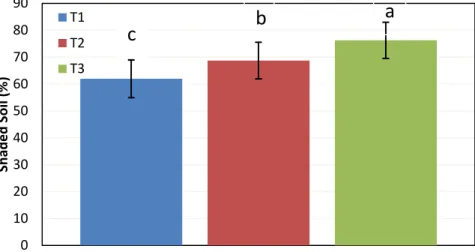
Regarding canopy development and size along the growing season, variance between treatments was highly significant, registering higher shaded soil % and m²of soil shaded per vine in treatment 3 at the end of the growing season compared to the rest of the treatments, and lower levels for T1, suggesting a higher canopy growth and canopy size in box pruning in contrast with spurs (Table 6 and Figure 19). These results are not surprising taking into account the higher crop load and buds left in the plant in T3 after winter pruning along with higher leaf area.

A bigger canopy shade beneath the canopy size would lead to a higher leaf area as shown in similar studies (Williams and Ayars 2005), suggesting indirectly higher photosynthetic activity of the plant. This fact would imply a greater potential capacity to ripe higher yields, having special relevance taking into account final yields collected from each treatment shown in the following lines. Nevertheless further analysis would have been desirable since 81-91% of total photosynthesis is made by the external layer of the canopy or the external exposed area with greater sunlight exposure (Smart 1985). In fact, at some point, the increase of canopy density would not be favorable for the grapevine microclimate lowering significantly photosynthetic capacity (Smart 1973; Schneider 1989).

33

T1 T2 T3 Significance

Shaded soil (m²/vine) 2.0 c 2.3 b 2.5 a ***

Shaded soil (%) 62 c 69 b 76 a ***

Table 6 : Shaded soil results at harvest time (T1= treatment 1(spur pruning 14 buds per vine to reach 10 shoots per row); T2= treatment 2(spur pruning 14 buds per vine to reach 10 shoots per row and no shoot removal); T3= treatment 3 box pruning (3 buds per spur and in general

around 21 buds per vine and no shoot removal). ns=not significant ;*,**and*** represent

significance at P=0,05,0,01 and 0,001 levels respectively; Figures for different treatments, followed by the same letter, do not differ significantly at p≤0.05).

Figure 19: Shaded Soil % comparison between treatments at the end of the growing season with standard error (T1= treatment 1(spur pruning 14 buds per vine to reach 10 shoots per row); T2= treatment 2(spur pruning 14 buds per vine to reach 10 shoots per row and no shoot removal); T3= treatment 3 box pruning (3 buds per spur and in general around 21 buds per vine and no shoot removal). Figures for different treatments, followed by the same letter, do not differ significantly at p≤0.05).

Canopy size and photosynthesis rates have a critical effect on water use showing a linear relation between water use by the plant and the shade cast on the ground (Williams and Ayars 2005). In fact, T3 required more than double the volume of irrigation water than T1 representing an important impact in the production costs in water and electricity (Table 7)(rain water was not taken into account since the same amount was spread equally among the 3 treatments). 0 10 20 30 40 50 60 70 80 90 Shaded Soil (% ) T1 T2 T3

c

b

a

34 In contrast, Water efficiency was significantly higher in T3 compared to hand pruning since liters of water required per kg of grapes produced was lower in T3 (Figure 20 and Table 7). This observation reveals that, even with higher water requirements per plant, T3 showed a more efficient water use than traditional spur pruning, and consequently more water sustainability. Same tendency was obtained by Botha 2013 in the same parcel. However, some authors have described lower water efficiency in the most irrigated treatment (Medrano et al 2014), more particularly if the yield was regulated by the legislation. In this study case, optimized results for each treatment were purchased, that is why water efficiency represents the optimum for the training system.

Figure 20: Water Efficiency comparison between treatments with standard error (T1= treatment 1(spur pruning 14 buds per vine to reach 10 shoots per row); T2= treatment 2(spur pruning 14 buds per vine to reach 10 shoots per row and no shoot removal); T3= treatment 3 box pruning (3 buds per spur and in general around 21 buds per vine and no shoot removal). Figures for different treatments, followed by the same letter, do not differ significantly at p≤0.05). 0 20 40 60 80 100 120 140 160 180 Water Effi ciency (L/kg) t1 T2 T3 a b b

35

T1 T2 T3 Significance

Irrigation Water(mm) 165 193 229

Yield (t/ha) 11.9 a 19.7 b 27.8 c **

Yield (kg/m²) 1.2 a 2.0 b 2.8 c **

Water Efficiency(L water/kg) 138 a 97 b 82 b **

Table 7: Yield and water efficiency results at harvest time (T1= treatment 1(spur pruning 14 buds per vine to reach 10 shoots per row); T2= treatment 2(spur pruning 14 buds per vine to reach 10 shoots per row and no shoot removal); T3= treatment 3 box pruning (3 buds per spur and in general around 21 buds per vine and no shoot removal). ns=not significant; ** represents significance at P=0,01 levels; Figures for different treatments, followed by the same letter, do not differ significantly at p≤0.05).

Significant differences were found between all the treatments concerning yield. T3 yielded 2.3 and 1.41 more than T1 and T2 respectively, reaching some times more than 30 tons per ha in few sub parcels. Yield differences could be explained by the number of clusters per plant which were highly superior in T3 compared to T2 and even more to T1, but cluster size was clearly smaller in T3 than in the other treatments. Similar results have been observed in different studies where box pruning showed significantly higher yields compared to manual pruning (De Toda 1999,Lopes et al 2000; Cruz et al 2010). Results show the great potential of the box pruning in terms of mass production (Table 7).

2. Must composition responses

Trend concerning technological ripeness parameters during berry development is well known (Deloire 2011, Keller 2010). Sugars accumulate via phloem water quickly inside the berry starting from early veraison, reaching a maximum threshold at the end of the ripening period. Meanwhile, pH increases and total acidity decreases respectively (Coombe 1987, Kennedy 2008) In this study, the pattern was kept, but clear differences between treatments were registered for the same parameters along the berry ripening period, from early veraison until full maturation(Figures 21, 22 and 23). Furthermore, total soluble solids, showed highly significant differences between all the treatments at late veraison (Figure 21).

In this case the delay in ripeness of T3 compared to the other treatments was even clearer in all the parameters but more accentuated in Total Soluble Solids. These results agree with the ones described by other authors showing the retarding effect on berry ripeness in minimal/box pruned vines (Sommer and Clingeleffer1993).

Figure 21 :Total Soluble solids evolution

(T1= treatment 1(spur pruning

2(spur pruning 14 buds per vine to reach 10 shoots per row and no shoot removal) treatment 3 box pruning (3 buds per spur and in general around 21 buds per vine and no shoot removal). ns=not significant ;*, ** and ***represent significance at P=0,05,0,01 and 0,001 levels respectively; Figures for different treatments, followed by the

significantly at p≤0.05). 0 5 10 15 20 25 30 800 1000 Total Sol uble Solids (ºbrix) T1 T2 T3 a ab b 2,0 2,5 3,0 3,5 4,0 800 1000 pH T1 T2 T3 ns c b a **

Figure 21 :Total Soluble solids evolution

Figure 22 : pH evolution

T1= treatment 1(spur pruning 14 buds per vine to reach 10 shoots per row)

14 buds per vine to reach 10 shoots per row and no shoot removal) 3 buds per spur and in general around 21 buds per vine and no shoot ns=not significant ;*, ** and ***represent significance at P=0,05,0,01 and 0,001 levels respectively; Figures for different treatments, followed by the same letter, do not differ

1200 1400 1600 1800 GrowingDegreeDays(ºC) a a b a b c ** a b c a a b a b b a b b a b *** *** 1200 1400 1600 1800 Growing DegreeDays(ºC) ns a a b a a b a a b a a b ns ns 36

14 buds per vine to reach 10 shoots per row); T2= treatment 14 buds per vine to reach 10 shoots per row and no shoot removal); T3= 3 buds per spur and in general around 21 buds per vine and no shoot ns=not significant ;*, ** and ***represent significance at P=0,05,0,01 and 0,001 same letter, do not differ

1800 2000

37

Figure 23 : Titratable acidity evolution

(T1= treatment 1(spur pruning 14 buds per vine to reach 10 shoots per row); T2= treatment 2(spur pruning 14 buds per vine to reach 10 shoots per row and no shoot removal); T3= treatment 3 box pruning (3 buds per spur and in general around 21 buds per vine and no shoot removal). ns=not significant ;*, ** and ***represent significance at P=0,05,0,01 and 0,001 levels respectively; Figures for different treatments, followed by the same letter, do not differ significantly at p≤0.05).

At harvest, small differences were registered between treatments in all the parameters above described (Table 8). T3 resulted, with a short significance, to induce lower pH, titratable acidity Total Soluble Solids than T1. Results on these aspects are still under debate in the literature (Schultz et al 2000, Poni et al 2000). However no differences were found in terms of Free Amino Nitrogen suggesting a correct performance of the Nitrogen soil treatment which was applied searching to optimize nitrogen requirements for each treatment at the beginning of the growing season.

Despite of the cited differences, all the parameters ranged within the standards for well ripened berries and compatible for a correct fermentation (Ribéreau Gayon 2006; Keller 2010). In fact, levels of FAN were in all the treatments higher than the threshold recommended we could expect that there are enough nutrients for the yeasts during a hypothetical fermentation of any of the resulting musts.

0 5 10 15 20 25 30 35 40 45 50 800 1000 1200 1400 1600 1800 2000 TA(g tartar ic acid/L) Growing DegreeDays(ºC) T1 T2 T3 ns ns ns b b a b b a b a a b b a _ns ** * ** **

38

T1 T2 T3 significance

pH 3.6 a 3.5 b 3.5 b *

Total Soluble Solids (ºbrix) 25.5 a 24.9 a 24.1 b *

Titratable Acidity (gTH2/L) 5.0 a 4.1 b 4.3 b *

Free Amino Nitrogen (mg/L) 264.9 265.4 264.3 Ns

DOY(day of the year) 250 c 257 b 275 a ***

Table 8 : Technological ripeness parameters at harvest (T1= treatment 1(spur pruning 14 buds per vine to reach 10 shoots per row); T2= treatment 2(spur pruning 14 buds per vine to reach 10 shoots per row and no shoot removal); T3= treatment 3 box pruning (3 buds per spur and in general around 21 buds per vine and no shoot removal). ns=not significant ;*,**and*** represent significance at P=0,05,0,01 and 0,001 levels respectively; Figures for different treatments, followed by the same letter, do not differ significantly at p≤0.05).

Concerning phenolic ripeness parameters at harvest, no significant differences were registered between treatments related with Total phenolic Index and Total Anthocyanins (Table 9). Furthermore, no variation was seen between T1 and T3 in terms of Mp%; Extractable Anthocyanins and extractablity %.

T1 T2 T3 significance

Total phenol Index 74 62 69 ns

Total Anthocyanins (mg malvidine/L) 1017 820 920 ns

Extractable Anthocyanins (mg malvidine/L) 674 a 489 b 653 a *

Extractability (%) 33 a 40 b 29 a *

Seed ripeness (Mp%) 63 b 68 a 61 b *

Day of the Year 249 a 256 b 273 a ***

Table 9: Phenolic ripeness parameters results at harvest (T1= treatment 1(spur pruning 14 buds per vine to reach 10 shoots per row); T2= treatment 2(spur pruning 14 buds per vine to reach 10 shoots per row and no shoot removal); T3= treatment 3 box pruning (3 buds per spur and in general around 21 buds per vine and no shoot removal). ns=not significant;*and*** represent significance at P=0,05 and 0,001 levels respectively; Figures for different treatments, followed by the same letter, do not differ significantly at p≤0.05).

Ribéreau-Gayon (2000) estated that Total Anthocyanins in must for Merlot cultivar are variable among seasons but the values ranges from 1012 and 1450 mg/L. In addition anthocyanin extractability (%) would range between 57 % and 85 % increasing with maturity. Finally, Total phenol index in wine ranges from 50 to 60. Results seems to be in general slightly below those ranges except for TPI suggesting that the year of study have had an effect on the results. In terms of phenolic ripeness, it can be said that no significant differences were found between T1 and T3.

39 Figure 24 represents the evolution of the anthocyanins extractability and tannin content in the seeds through the ripening period. Mp% seems to have a decreasing trend in all he treatments suggesting a lower accumulation of tannins in the berry when the berries are riper. In contrast, extractable anthocyanins and extractability % suffered and increase during maturity in all the treatments. Similar results were described by Glories 2001.

40

Figure 24: tannins content in the seeds (A) and Ant. Extractability (B; C) through berry ripening (T1= treatment 1(spur pruning 14 buds per vine to reach 10 shoots per row); T2= treatment 2(spur pruning 14 buds per vine to reach 10 shoots per row and no shoot removal); T3= treatment 3 box pruning (3 buds per spur and in general around 21 buds per vine and no shoot removal).

y = -2,617x + 134,9 R² = 0,992 y = -2,497x + 128,7 R² = 0,975 y = -3,130x + 134,4 R² = 0,905 40 50 60 70 80 90 100 14 16 18 20 22 24 26 28 Seeds ripen ess (%M p)

Total Soluble Solids (ºbrix)

T1 T2 y = 19,39x + 30,28 R² = 0,982 y = 11,42x + 187,5 R² = 0,632 y = 37,43x - 227,1 R² = 0,922 300 350 400 450 500 550 600 650 700 750 14 16 18 20 22 24 26 Extractab le A nth ocyanin ( mg malvidine /L)

Total Soluble Solids (ºBrix)

T1 T2 T3 10 15 20 25 30 35 40 45 50 1300 1400 1500 1600 1700 1800 1900 2000 Extractab ili ty %

Growing Degree Days(ºC)

T1 T2 T3 A B C