CINTAL - Centro de Investiga¸
c˜
ao Tecnol´
ogica do Algarve
Universidade do Algarve
Vector Sensor Array Data Report
Makai Ex 2005
P. Santos
Rep 02/08 - SiPLAB March/2008
University of Algarve tel: +351-289800131 Campus de Gambelas fax: +351-289864258
8005-139 Faro, [email protected]
Work requested by CINTAL
Universidade do Algarve, FCT - Campus de Gambelas 8005-139 Faro, Portugal
Tel/Fax: +351-289864258, [email protected], www.ualg.pt/cintal
Laboratory performing SiPLAB - Signal Processing Laboratory
the work Universidade do Algarve, FCT, Campus de Gambelas, 8000 Faro, Portugal
tel: +351-289800949, [email protected], www.siplab.fct.ualg.pt
Projects
Title Vector Sensor Array Data Report Makai Ex 2005 Authors P. Santos
Date March, 2008 Reference 02/08 - SiPLAB Number of pages 38 (thirty eight)
Abstract This report describes the data acquired with a Vector Sen-sor Array (VSA) during the Makai Ex 2005, that took place aboard the R/V Kilo Moana from 15 September to 2 October, 2005, off the coast of Kauai I. (Hawai), United States. The orientation of the axis on VSA, a study of direction of arrival estimation and bottom properties estimation are included. Clearance level UNCLASSIFIED
Distribution list SiPLAB(1), CINTAL (1) Total number of copies 2 (two)
Contents
List of Figures V
Abstract 7
1 Introduction 9
2 The Makai Experiment 2005 Sea Trial 10
2.1 Bottom data . . . 10
2.2 Water column data . . . 10
2.3 Deployment Geometries . . . 13
2.3.1 Julian Day 264 . . . 13
2.3.2 Julian Day 267 . . . 15
2.3.3 Julian Day 268 . . . 15
3 Vector Sensor Array in MakaiEx 18 3.1 Emitted signals . . . 20
4 Direction of Arrival Estimation with VSA 22 4.1 Vector Sensor Array Beamforming . . . 22
4.2 Beamforming of ship noise . . . 23
4.3 Acoustic Sources DOA Estimation . . . 24
4.3.1 Julian Day 264 . . . 28
4.3.2 Julian Day 267 . . . 28
4.3.3 Julian Day 268 . . . 29
5 Bottom Properties Estimation 31 5.1 Bottom Reflection Coefficient . . . 31
IV CONTENTS 5.2 Analisys of Results . . . 32 6 Conclusion and future work 37
List of Figures
2.1 Makai Experiment site off the north west coast of Kauai I., Hawaii, USA. . 11 2.2 Bathymetry map of the area and the location of the acoustic sources TB1
and TB2, thermistor strings TS2 and TS5, XBT and XCTD. . . 11 2.3 Recorded XBT (red) and XCDT (blue) casts: temperature profiles (a) and
sound velocities profiles (b). . . 12 2.4 Thermistor strings temperature data recordes on: TS2 (a) and TS5 (b). . . 12 2.5 Sound speed profiles during Julian Day 264 and mean sound speed profile
(thick line). . . 13 2.6 Bathymetry map of the area and location of the acoustic sources TB1, TB2
and the VSA on Julian day 264. . . 14 2.7 Bathymetric profile between the VSA: and TB1 (a) and TB2 (b). . . 14 2.8 Bathymetry map of the area and the location of the acoustic source TB2
and VSA drift on Julian day 267. . . 15 2.9 Bathymetric profile (a) and source - receiver range (b) during Julian day
267. . . 16 2.10 The location of VSA and RHIB track during part of Julian day 268. . . 16 2.11 Bathymetric profile (a) and source - receiver range (b) between VSA and
Lubell source, during Julian day 268. . . 17 3.1 Constitution of a single vector sensor and x, y and z axis orientation. . . . 19 3.2 A 5 element vertical VSA: hose (a) and 10 cm element spacing view (b). . 19 3.3 Received probe signals on VSA transmitted by the acoustic sources: TB1
(a) and TB2 (b). . . 20 3.4 Received signal on VSA by Lubell source. . . 21 4.1 Array coordinates and geometry of acoustic plane wave propagation. . . 23 4.2 Spectogram of noise generated by R/V Kilo Moana on pressure sensor of
VSA at 79.6m on Julian day 264. . . 24 V
VI LIST OF FIGURES 4.3 Power spectrum (1s averaging time) of noise generated by R/V Kilo Moana
on Julian day 264, on vector sensor at 79.6m on: pressure sensor (a), x component (b), y component (c) and z component of velocity sensors (d). . 25 4.4 Real data beamforming results for the frequency of 300Hz: estimated
am-biguity surface (a) and azimuth estimation during period of aquisition on Julian day 264 (b), 267 (c) and 268 (d). . . 26 4.5 Heading data from ship’s instruments on days: 264 (a), 267 (b) and 268
(c) and Orientation of x and y-axis of the VSA in relation to Kilo Moana’s heading on days: 264 (d), 267 (e) and 268 (f ). . . 27 4.6 Real data beamforming results for frequency 8258 Hz: (a) ambiguity surface
at minute 3 for TB2 and (b) estimates of the azimuth during period of acquisition, for TB1(blue asterisk) and TB2(red triangle); green symbols represent outliers. . . 28 4.7 Real data azimuth estimation on Julian day 267, for tone at frequency:
8250 Hz (a) and 9820 Hz (b). . . 29 4.8 Real data results for the tone 6551 Hz ambiguity surface at minute 4
(be-ginning of data acquisition) (a) and estimated azimuths during the period of acquisition (b). . . 30 4.9 Makai experiment geometry on Julian day 268, track of the RHIB and x
and y axis orientation on VSA in respect to Lubell bearing estimation. . . . 30 5.1 The ray approach geometry of a plane wave emitted by the source (S) and
received by the receiver (R) at the steer elevation angle θ0 . . . 31
5.2 Beam response at source azimuthal direction φ = 14o, on Julian day 268
at minute 38, obtained using: 4 omni sensors (a) and all elements of the VSA (b). . . 32 5.3 Experimental drawing diagram of baseline environment with sound speed
profile on Julian day 268. . . 33 5.4 Spectrogram of 5s of LFM signal acquired by the VSA on Julian day 268 at
minute 38. . . 34 5.5 Bottom reflection loss calculated as the up-to-down ratio of the array
eleva-tion beams at minute 38 at range of approximately 500m (a) and at minute 48 at range of approximately 300m (b). . . 34 5.6 Reflection loss modelled by Safari model, with two estimated parameters:
poor attenuation in the sediment (a) and higher attenuation in the sediment (b). . . 35 5.7 Bottom reflection loss deduced from the up-to-down ratio of the beams at
minutes: 19 (a) and 27 (b), for Julian day 264 and TB2 at range of 1830m. 36 5.8 Bottom reflection loss deduced from the up-to-down ratio of the beams at
Abstract
The purpose of the MakaiEx sea trial was to acquire data over a large range of frequen-cies from 500 Hz upto 50 kHz, for a variety of applications ranging from high-frequency tomography, coherent SISO and MIMO applications, vector sensor and active and passive sonar, etc. The MakaiEx sea trial took place off the coast of Kauai I., Hawai, from 15 September to 2 October, 2005, involving a large number of teams both from government and international laboratories, universities and private companies, such as HLS Research, UDEL, SPAWAR, NRL and SiPLAB. MIMO, Acoustical Oceanographic Buoy (AOB), Acoustic Communications and Data Storage, Acoustic sources Testebs, Gliders and Vec-tor Sensor Array (VSA) were some of the equipment that was deployed during Makai and some of them served multiple purposes. This report describes the data acquired with the VSA as well as all the related environmental and geometrical data relative to the VSA deployments. It is also described a preliminary VSA data processing aiming at direction of arrival estimation for low frequency ship noise and high frequencies signals emitted by controlled acoustic sources. The estimation of bottom properties, using a method that consists in dividing downward by upward beam response, is also discussed. The bottom reflection loss deduced from experimental data is compared to the modelled reflection loss using the SAFARI model.
8
Chapter 1
Introduction
Vector sensors measure the acoustic pressure and the particle velocity components, and are normally configured as vector sensor arrays (VSA). This type of sensor has the ability to provide information in both vertical and azimuthal direction and start to be available for underwater acoustic applications. The spatial filtering capabilities of a VSA can be used, with advantage over traditional pressure only hydrophones arrays, for source local-ization and for estimating acoustic field directionality as well as arrival times and spectral content, which open up the possibility for its use in sea bottom properties estimation. An additional motivation of this work is to test the possibility of using high frequency probe signals (say above 2 kHz) for reducing size and cost of actual sub bottom profilers and adequate geoacoustic inversion methods. It will be demonstrated the advantages of using a VSA in source localization and bottom properties estimation by using a method that obtain the bottom reflection coefficient as the ratio between the upward and downward VSA real data beam response [1]. This document attempts to make a complete report of the various data sets acquired by the VSA during the MakaiEx sea trial between 15 September and 2 October, as well as other data such as ship’s and VSA position, temper-ature and sound velocity profiles and geo-acoustic information. In that sense this report complements the Acoustic Oceanographic Buoy (AOB) Data Report [2], that describes only the AOB2 data set.
This report is organized as follows: chapter 2 makes a short description of the Makai Experiment 2005 sea trial when the VSA was deployed, including the non-acoustic mea-surements, bathymetry and geometry information; chapter 3 describes the actual VSA used during the sea trial as well as the emitted signals; chapter 4 describes the direction of arrival estimation for low and high frequencies and related theory of VSA beamforming; chapter 5 describes the bottom properties estimation and finally chapter 6 concludes this report giving some hints for future work.
Chapter 2
The Makai Experiment 2005 Sea
Trial
The MakaiEx sea trial took place off the coast of Kauai I., Hawai, from 15 September to 2 October 2005 and was the third experiment specifically planned to acquire data to support the High-Frequency initiative (HFi). The HFi involves a wide spectrum of objectives that reflect specific interests such as: high-resolution tomography, acoustic propagation model-ling in the high frequency range, understanding of the acoustic-environment interaction at high frequencies and its influence on underwater communications. Organized by HLS Research and financed by ONR, involved a large number of teams both from government and international laboratories, universities and private companies, such as HLS, UALg, UDEL, SPAWAR, NRL, NURC. The selected area for the MakaiEx sea trial is shown in Fig. 2.1 and is well documented in [2]. The purpose of this chapter is to provide a short description of the data acquired by the VSA as well as the related environment and geometrical data relative to the VSA deployments in MakaiEx.
2.1
Bottom data
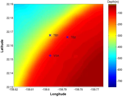
Extensive ground truth measurements were carried out in this area during previous ex-periments and showed that most of the bottom surface of the area is covered with coral sands over a basalt hard bottom. The sound velocity in coral sands should be approxi-mately 1700 m/s and the sediment thickness is unknown but expected to be a fraction of a meter in most places according to previous sidescan surveys. It is expected that coral sands cover most of the plateau around the Kauai I. Fig 2.2 shows the localization of some environmental recording equipment and the bathymetry of the area, where it can be seen an almost smooth and uniform area of constant depth around 80-100m accompanying the island bathymetric contour surrounded by the continental relatively steep slope to the deeper ocean to the West.
2.2
Water column data
During MakaiEx a number of environmental recording equipment was deployed, in at-tempt to collect as much environmental data as possible, mostly aiming at the water column variability, that included two thermistor strings, (TS2 and TS5) and XBTs and
2.2. WATER COLUMN DATA 11
Figure 2.1: Makai Experiment site off the north west coast of Kauai I., Hawaii, USA.
Figure 2.2: Bathymetry map of the area and the location of the acoustic sources TB1 and TB2, thermistor strings TS2 and TS5, XBT and XCTD.
12 CHAPTER 2. THE MAKAI EXPERIMENT 2005 SEA TRIAL
(a) (b)
Figure 2.3: Recorded XBT (red) and XCDT (blue) casts: temperature profiles (a) and sound velocities profiles (b).
(a) (b)
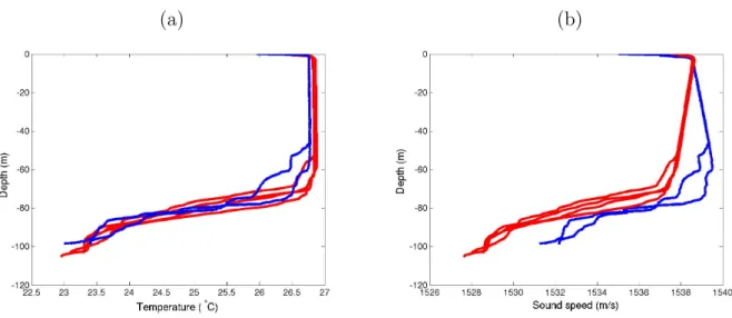
Figure 2.4: Thermistor strings temperature data recordes on: TS2 (a) and TS5 (b). XCTDs recordings. The localization of the acoustic sources testbeds TB1 and TB2, ter-mistors strings TS2 and TS5, XBT and XCTD are shown in Fig. 2.2. The measured temperature profiles and calculated sound velocities obtained from XBT and XCTD are shown in Fig. 2.3, red and blue lines respectively.
Several thermistor strings were deployed but due to the adverse weather conditions encountered during the first days of the sea trial, only the thermistor strings TS2 and TS5 were recovered with successful data recordings. The recorded temperatures are shown in Fig. 2.4, for: TS2 (a) and TS5 (b). Fig. 2.5 shows the variability of sound speed profile during Julian Day 264 and the thick line is the mean sound speed profile used for data processing.
2.3. DEPLOYMENT GEOMETRIES 13
Figure 2.5: Sound speed profiles during Julian Day 264 and mean sound speed profile (thick line).
VSA Start time End time
Local time Julian day Local time Julian day Deployment 1 20/09/05; 19:20 264.22 21/09/05; 05:30 264.5 Deployment 2 23/09/05; 19:00 267.21 23/09/05; 22:10 267.34 Field Calibration 25/09/05; 08:30 268.77 25/09/05; 10:22 268.85 Table 2.1: Schedule time of VSA deployments during MakaiEx, local times and Julian days.
2.3
Deployment Geometries
A note should be made here regarding the convention used for converting actual calendar UTC date and time to UTC Julian time. In this report and in agreement with the on board master clock the former has been used, so day September 15, 2005 02:00 local time will be coded as Julian time 258.5 UTC.
The VSA was deployed during three periods of time, fairly close to the stern of R/V Kilo Moana and tied to a vertical cable. Three data sets were acquired: one on Julian Day 264; another on Julian Day 267 and a third and last recording on Julian Day 268, during the Field Calibration test (see Table 2.1).
14 CHAPTER 2. THE MAKAI EXPERIMENT 2005 SEA TRIAL Deployment Lat Long WD SD Distance
(m) (m) to VSA (km) TB1 2 22.1675N -159.7977W 265 201.5 1.634 TB2 1 22.1661N -159.7870W 104 98.2 1.830
Table 2.2: Locations and geometric characteristics of acoustic sources, TB1 and TB2; last columns show estimated source depth (SD) and estimated source range between the acoustic sources and VSA.
Figure 2.6: Bathymetry map of the area and location of the acoustic sources TB1, TB2 and the VSA on Julian day 264.
(a) (b)
2.3. DEPLOYMENT GEOMETRIES 15
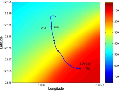
Figure 2.8: Bathymetry map of the area and the location of the acoustic source TB2 and VSA drift on Julian day 267.
On day 264, corresponding to the first VSA deployment, both acoustic sources TB1 and TB2 were bottom moored. The VSA was fixed at 80m depth in a water depth of approximately 104m and deployed at latitude 22.1526N and longitude -159.7976W. The locations and geometric characteristics of acoustic sources are given in Table 2.2. The bathymetry map of the area on Julian Day 264 is shown in Fig. 2.6. The bathymetric contours between VSA and TB1 was range dependent and between VSA and TB2 was approximately range independent, as shown in Fig. 2.7 (a) and (b), respectively.
2.3.2
Julian Day 267
The second VSA deployment took place on day 267. Only acoustic source TB2 was transmitting, deployed at location 22.1660N,-159.7870W and depth 89.5m in 104m water depth. During this day R/V Kilo Moana, with the VSA at the stern at 40m depth, drifted from the TB2 location to a position 22.1889N and -159.7968W, corresponding to an approximate distance of 2.3 km. The drift of the VSA and the location of TB2 are shown in Fig. 2.8. The bathymetric profile and source - receiver range are shown in Fig.2.9 (a) and (b).
2.3.3
Julian Day 268
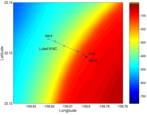
The third and last VSA deployment ocurred on day 268. This day was dedicated to ”Field Calibration” operations and the signals were transmitted by the acoustic source Lubell 916C3. The source was being towed by the RHIB at 10m depth and the VSA was fixed at
16 CHAPTER 2. THE MAKAI EXPERIMENT 2005 SEA TRIAL
(a) (b)
Figure 2.9: Bathymetric profile (a) and source - receiver range (b) during Julian day 267.
2.3. DEPLOYMENT GEOMETRIES 17
(a) (b)
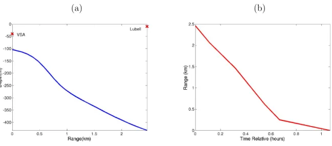
Figure 2.11: Bathymetric profile (a) and source - receiver range (b) between VSA and Lubell source, during Julian day 268.
location 22.1478N and -159.80W at 40m depth. The VSA location and the RHIB track are shown in Fig. 2.10. The bathymetric cut along track and source - receiver range, between the Lubell source and the VSA are shown in Fig.2.11 (a) and (b), respectively.
Chapter 3
Vector Sensor Array in MakaiEx
Historically, ocean acoustic signals have been recorded using hydrophones, that measure the pressure field and are typically omnidirectional. Recent studies and developments in piezoelectric materials have led to the use of vector sensors in many underwater appli-cations with a significant improvement in performance [3]. Vector sensors measure the acoustic pressure and the particle velocity components and this type of sensors, assem-bled into an array, has the ability to provide information in both vertical and azimuthal directions allowing increased directivity. The VSA used during the Makai Experiment was constituded by sensors of type TV-001, constructed by Wilcoxin Corporation with one omnidirectional pressure sensor (hydrophone) and three accelerometers arranged in a triaxial configuration and mounted in a neutrally buoyant package approximately 3.81cm in diameter and 6.35cm long, Fig. 3.1.
During the MakaiEx sea trial a 5 element vertical VSA, Fig. 3.2, with 10 cm spacing between each element, was used to collect data from towed and fixed acoustic sources. The VSA was deployed fairly close to the stern of R/V Kilo Moana and tied to a vertical cable, with a 100-150 kg weight at the bottom, to ensure that the array stayed as close to vertical as possible. Each element of the VSA produces four time series streams of data, one for the pressure hydrophone and three for the particle velocity outputs. Therefore, 5 elements produce 20 channels of time series data. Unfortunately, the 5th element didn’t work, as a result only 16 channels of time series were acquired. The order of the channels is:
• channel 1 – pressure for element 1;
• channel 2 – velocity in X direction at element 1; • channel 3 – velocity in Y direction at element 1; • channel 4 – velocity in Z direction at element 1; • channel 5 – pressure for element 2;
• channel 6 – velocity in X direction at element 2; and so on.
19
Figure 3.1: Constitution of a single vector sensor and x, y and z axis orientation.
(a) (b)
20 CHAPTER 3. VECTOR SENSOR ARRAY IN MAKAIEX
(a) (b)
Figure 3.3: Received probe signals on VSA transmitted by the acoustic sources: TB1 (a) and TB2 (b).
3.1
Emitted signals
Acoustic signals received by the VSA were emitted from a variety of sound sources that included the two testbeds TB1 and TB2 and the Lubell 916C3 source. The frequency band of the transmitted signals was 8 - 14kHz for the fixed testbeds and 500 - 14000Hz for the Lubell source towed by the RHIB boat. There was a variety of signals transmitted during the MakaiEx sea trial that included two phases:the Probes and Comms (PC) phase and the Field Calibration (FC) phase.
During the PC phase the two testbeds transmitted alternatively every 2 minutes, both with allocated time slots to the various research teams on board, as explained in chapter 4 of [2]. Each 2 minutes data block has one probe signal with 10s time duration, common to all data blocks of all institutions and then 107s of communication signals (different for each institution). The common probe signal, Fig. 3.3, has a total duration of 10s and has three sub regions, having different signals for each testbed:
1. The first region is occupied by LFM upsweeps between 8 and 14kHz with 50ms time duration and 200ms of silence between them, during 4s;
2. The second region is occupied by a multitone signal, with 8 tones in the 8-14kHz band with a duration of 2s, and where each source has a specific set of frequencies: 8250, 8906, 8976, 11367, 11789, 12774, 13055 and 13992Hz for TB1 and 8250, 9820, 9914, 11367, 11789, 11882, 13078 and 13500Hz for TB2, so this can be used to differentiate the two testbeds;
3. The third region contains a 4s-long M-sequence centered at 11kHz with a 3000chips/s bit rate.
During the FC phase, a much wider frequency band was explored thanks to the trans-missions characteristics provided by the Lubell source towed from the RHIB. The signal is a sequence of LFM’s, multitones and M-sequence in the 500 - 14000Hz band, as shown in Fig. 3.4. The FC sequence has 2 minutes of duration, constituded by:
1. A first region is occupied by 6s of LFM and 8s of M-sequence in 8-14kHz band; 2. A second region is occupied by 6s of LFM and 30s of M-sequence in 1.5-9kHz band;
3.1. EMITTED SIGNALS 21
Figure 3.4: Received signal on VSA by Lubell source.
3. The third region contains 10s of Multitones with the frequenies: 950Hz, 1311Hz, 1810Hz, 2498Hz, 3444Hz, 4750Hz, 6544Hz and 9027Hz;
Chapter 4
Direction of Arrival Estimation with
VSA
The estimation of directional of arrival (DOA) of an acoustic wave is usually performed with traditional scalar (pressure only) hydrophones. However, recent studies suggest that vector sensors could improve source localization and provide information in both vertical and azimuthal directions [4]. The main advantage of the VSA is that it captures more acoustic information, hence it provides substantially higher directivity with a much smaller aperture than an array of traditional scalar hydrophones.
The discussion of DOA estimation using a VSA with traditional beamformer and the advantages that these new sensors provide over conventional pressure only arrays were presented in [5]. Here, the real data results of DOA estimation for the three deployments of the VSA during MakaiEx are shown.
4.1
Vector Sensor Array Beamforming
To resolve the DOA estimation using a VSA, the plane wave beamformer is applied, where the individual sensor outputs are delayed, weighted and summed in a conventional manner. A single vector sensor outputs has four measured quantities given by:
Vn = [pn, vxn, vyn, vzn] , (4.1)
where pn is the scalar pressure and vxn, vyn and vzn are the three components of particle
velocity at the nth element of the VSA.
Several approaches to beamforming were presented in [6], but here a weighting vector, w, that uses direction cosines as weights for the velocity components and an unit weigth for pressure, has been chosen. Thus for the nth element, the weigthing vector is given by:
wn = [wpn, wxn, wyn, wzn]
= [1, cos(θS) sin(φS), sin(θS) sin(φS), cos(φS)] · exp(i
− →
kS· −→rn), (4.2)
where n = 1, · · · , N , N is the number of elements in VSA, −→kS is the wave number vector
corresponding to the chosen steered, or look direction (θS, φS), of the array and −→rn is the
position vector of the nth element, Fig. 4.1. 22
4.2. BEAMFORMING OF SHIP NOISE 23
Figure 4.1: Array coordinates and geometry of acoustic plane wave propagation. The array elements are equally spaced and located along the z-axis, with the first one in the origin of the cartesian coordinates system, Fig. 4.1, thus −→rn = [0, 0, zn]. For a VSA
with N elements, the weigthing vector W is of dimension 4N × 1 and is defined as: W(θS, φS) = [w1, w2, · · · , wN] . (4.3)
The general expression for the beamformer in direction (θS, φS) is given by:
B(θS, φS) = W(θS, φS) · R · WH(θS, φS), (4.4)
where R is 4N × 4N correlation matrix. Then, the azimuth and the elevation angles of the plane wave impinging on the array are estimated by finding the values (θS, φS) that
maximize (4.4).
4.2
Beamforming of ship noise
The VSA was deployed with the z-axis vertically oriented with respect to the bottom but the orientation of x and y-axis were unknown. In order to determine the VSA orientation in the horizontal plane, the acoustic signature of the R/V Kilo Moana combined with the its GPS data and heading was used.
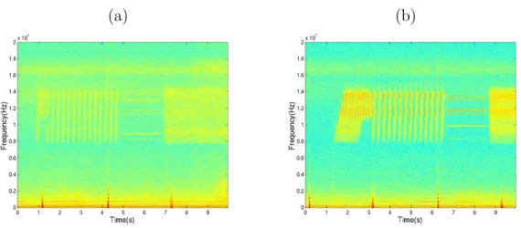
Observing the data collected by the VSA, at low frequency, the spectral characteristics of the signal are fairly stable over time for all days during which the VSA was deployed, Fig. 4.2. Two dominant frequencies, 180Hz and 300Hz, were observed in all output signals of the VSA (pressure and particle velocities components), as shown in Fig. 4.3. These were assumed to be part of ship signature and used to find the orientation of the VSA in the horizontal plane. The correlation matrix, R, of (4.4) is estimated for each frequency using: ˆ R = 1 K K X k=1 Vk· VHk, (4.5)
24 CHAPTER 4. DIRECTION OF ARRIVAL ESTIMATION WITH VSA
Figure 4.2: Spectogram of noise generated by R/V Kilo Moana on pressure sensor of VSA at 79.6m on Julian day 264.
where K is the number of snapshots and the vector Vk represents the FFT bin at the
frequency of interest at the kth snapshot for all sensors, containing 16 VSA channels, 4
measured quantities from each of the four vector sensor elements.
Fig. 4.4 shows the results obtained when (4.4) and (4.5) were applied to the real data at the frequency of 300Hz. The ambiguity surface using real data is remarkably consistent for all days, with the peak at an azimuth of -134o and an elevation of -35o, Fig. 4.4 (a).
The estimated azimuths do not vary over the processing interval and one can conclude that the VSA was deployed with the same orientation facing the R/V Kilo Moana for all days, Fig. 4.4 (b), (c) and (d). Heading data from the ship’s instruments shows that R/V Kilo Moana, on Julian day 264, was heading approximately 50o with respect to
North, Fig. 4.5 (a). Thus one can conclude that the x-axis components of the VSA were oriented approximately to the South and the y-axis components to the West, Fig. 4.5 (e). The same conclusion were obtained for the Julian days 267 and 268. Fig. 4.5 shows the heading data from ship’s instruments for all days of VSA deployments on the left side and the x and y-axis orientation on the rigth side. Note that, on Julian day 267, the R/V Kilo Moana with the VSA at stern was drifting from location of TB2 to the North, then the orientation presented in Fig. 4.5 (e) is for the beginning of VSA data acquisition, when the R/V Kilo Moana was heading to 45o with respect to the North. So, the orientation of
x and y-axis changed during the drifting and is obtained aligning the ship’s heading with the arrows presented in Fig. 4.5 (e).
4.3
Acoustic Sources DOA Estimation
The DOA estimation results for the acoustic sources used the orientations of x and y-axis VSA components, estimated in previous section from the ship signature. The 4 element vertical VSA was located along the z-axis, with 10 cm element spacing, which is the half-wavelength spacing at a frequency of 7500Hz.
4.3. ACOUSTIC SOURCES DOA ESTIMATION 25
(a) (b)
(c) (d)
Figure 4.3: Power spectrum (1s averaging time) of noise generated by R/V Kilo Moana on Julian day 264, on vector sensor at 79.6m on: pressure sensor (a), x component (b), y component (c) and z component of velocity sensors (d).
26 CHAPTER 4. DIRECTION OF ARRIVAL ESTIMATION WITH VSA
(a) (b)
(c) (d)
Figure 4.4: Real data beamforming results for the frequency of 300Hz: estimated ambiguity surface (a) and azimuth estimation during period of aquisition on Julian day 264 (b), 267 (c) and 268 (d).
4.3. ACOUSTIC SOURCES DOA ESTIMATION 27
(a) (d)
(b) (e)
(c) (f)
Figure 4.5: Heading data from ship’s instruments on days: 264 (a), 267 (b) and 268 (c) and Orientation of x and y-axis of the VSA in relation to Kilo Moana’s heading on days: 264 (d), 267 (e) and 268 (f ).
28 CHAPTER 4. DIRECTION OF ARRIVAL ESTIMATION WITH VSA
(a) (b)
Figure 4.6: Real data beamforming results for frequency 8258 Hz: (a) ambiguity surface at minute 3 for TB2 and (b) estimates of the azimuth during period of acquisition, for TB1(blue asterisk) and TB2(red triangle); green symbols represent outliers.
4.3.1
Julian Day 264
The signals emitted by the two testbeds (TB1 and TB2), on Julian day 264, in the 8 -14 kHz band, are shown in Fig. 3.3. Beamforming was performed for 8 tones and each testbed had a distinst set of tones, where the only common frequency was 8258 Hz. The ambiguity surfaces for the multitones received on VSA from TB1 and TB2 are similar, but in different angles. Fig. 4.6 (a) shows the ambiguity surface obtained from TB2 at minute 3 for 8258 Hz tone and Fig 4.6 (b) presentes the azimuth estimation during the period of aquisition, for both sources: blue line for TB1 and red line for TB2. Since of all tones are above the design frequency of 7500 Hz of the array, there is some spatial aliasing and ambiguities in the directions of arrival are observed (green symbols in Fig. 4.6 (b)).
The relative angle between the estimated azimuths of sources TB1 and TB2, shown in Fig. 4.6 (b), does not vary and the fluctuation of the azimuth observed, during this interval, may be due to ship heading displacements or to the rotation of the VSA about the z-axis. However, these results are verified with the known Makai Experiment geometry shown in Fig. 4.5 (d), presented in previous section, and the DOA estimation is consistent with those results.
4.3.2
Julian Day 267
On Julian day 267, acoustic signals were emitted by the fixed source TB2 (see deployment 2 Table in 2.1)while the VSA was being suspended by R/V Kilo Moana (see drift on Fig. 2.8).
The VSA acquired almost 3 hours of data and the estimated azimuth, for two different frequency tones, are shown in Fig. 4.7. These estimates show that the orientation of the x-y plane on VSA changed with the drift of the R/V Kilo Moana and with respective rotation of her heading. The source bearing estimation is in line with the orientation of x and y axis at the beginning of VSA acquisition (near TB2) and then with its drift to North shown in Fig. 4.5 (e). There is some spatial aliasing and ambiguities in the directions of arrival, observed by the green symbols in Fig. 4.7.
4.3. ACOUSTIC SOURCES DOA ESTIMATION 29
(a) (b)
Figure 4.7: Real data azimuth estimation on Julian day 267, for tone at frequency: 8250 Hz (a) and 9820 Hz (b).
4.3.3
Julian Day 268
Julian day 268 was dedicated to ”field calibration” operations and the Lubell 916C3 source was being towed by the RHIB (in the morning). The emitted signals, shown in Fig. 3.4, were in the 500 Hz to 14 kHz band with some frequencies bellow the design frequency of the VSA. The tone used to estimate the azimuth was 6551 Hz, the nearest to the frequency 7500 Hz, with no spatial aliasing. The ambiguity surface at minute 4 and the azimuth estimation for almost one hour of data acquisition are shown in Fig. 4.8 (a) and (b), respectively. The ambiguity surfaces for the remaining acquisition period are similar to Fig. 4.8 (a) and, as it can be remarked, some ambiguity due to the proximity to the zero of the elevation angle may be observed, providing the green points in Fig. 4.8 (b). The last points in the 3rd quadrant are due to the sound source passed over the VSA location in direction to the south. These results are not in agreement with the orientation of x-y plane on VSA presented in Fig. 4.5 (f). The beamforming applied to all acquisition data from the Lubell source gave the same estimates. The orientation of x-y plane on VSA with respect to the Lubell bearing estimation is shown in Fig. 4.9 and present 90o
30 CHAPTER 4. DIRECTION OF ARRIVAL ESTIMATION WITH VSA
(a) (b)
Figure 4.8: Real data results for the tone 6551 Hz ambiguity surface at minute 4 (beginning of data acquisition) (a) and estimated azimuths during the period of acquisition (b).
Figure 4.9: Makai experiment geometry on Julian day 268, track of the RHIB and x and y axis orientation on VSA in respect to Lubell bearing estimation.
Chapter 5
Bottom Properties Estimation
The spatial filtering capabilities and directionality of the VSA, presented in section 4, provide a clear advantage in source localization and opens up the possibility for its usage in other type of applications such as in geoacoustic inversion. The objective of this section is to test the possibility of using a VSA for estimating bottom properties, specially bottom reflection coefficient, using a method proposed in [1]. Source bearing could be determined using the horizontal discrimination capability of the VSA and the corresponding beam extracted for vertical resolution analysis.
5.1
Bottom Reflection Coefficient
C. Harrison et al. [1] proposed an estimation technique, using vertical array measurements of surface generated noise, where an estimate of bottom reflection loss versus grazing angle for the signal bandwidth is obtained by dividing the down and upward energy reaching the array. This technique is addapted for vertical measurements of an azimuthal direction of acoustic sources with a small aperture vertical VSA, [7]. Let us consider an emitted signal S(φ, θ), in a range independent environment for an elevation angle θ and azimuth angle φ, Fig. 5.1. To estimate the array beam pattern B(φ, θ) for source look direction φ, plane wave beamforming was applied and the individual sensor outputs were delayed, weighted and summed in a conventional manner [5], considering a weighting vector that uses direction cosines as weights for the velocity components and an unit weight for the pressure. Then, the array beam pattern in azimuthal direction φ, for each steer elevation angle θ0 is given by the array response A(θ0). The ratio between the downward and
Figure 5.1: The ray approach geometry of a plane wave emitted by the source (S) and received by the receiver (R) at the steer elevation angle θ0
. 31
32 CHAPTER 5. BOTTOM PROPERTIES ESTIMATION
Figure 5.2: Beam response at source azimuthal direction φ = 14o, on Julian day 268 at minute 38, obtained using: 4 omni sensors (a) and all elements of the VSA (b).
upward beam response is an approximation to the bottom reflection coefficient Rb:
A(−θ0)
A(+θ0)
= Rb[θb(θ0)], (5.1)
where the angle measured by beamforming at the receiver, θ0, is corrected to the angle
at the seabed, θb, according to sound-speed profile by Snell’s law:
θb = acos[(
cb
cr
)cos(θ0)], (5.2)
where cb is the sound speed at the bottom and crthe sound speed at the receiver, according
to [1].
Dividing the down to upward beam response for the same elevation angle, the fre-quency versus bottom angle reflection losses curves are generated and then compared with reflection losses curves modeled by the SAFARI model, for a given set of parame-ters for sediment and/or bottom: compressional wave speed cp, shear wave speed cS,
compressional wave attenuation αp, shear attenuation αS and density ρ. The best
agree-ment gives an estimate of bottom layering structure together with its most characteristic physical parameters.
As a first step to find the bearing of the source (azimuth), conventional vector sensor beamforming was used. Then the vertical beam response for each frequency was extracted for the source bearing of interest, considering both: the 4 omnidirectional pressure sensors only and the 4 omni+directional elements of the VSA, Fig 5.2. As it can be seen, the beam response in the omni directional case is nearly symmetric for the negative and positive elevation angles (up and down respectively), the horizontal directivity of the acoustic field does not exist, conducting to poor information about the bottom attenuation. Comparing with the directional case, in Fig. 5.2 b), the vertical beam response clearly differentiates up and downward energy allowing due to the high horizontal and vertical directivity, retrieving bottom information. This is clearly an unique capability resulting from the processing gain provided by the VSA.
5.2
Analisys of Results
The first data analysed here were acquired by the VSA, on Julian day 268 (section 4.3.3), and emitted by acoustic source Lubell 916C3, towed from RHIB and deployed at 10m
5.2. ANALISYS OF RESULTS 33
Figure 5.3: Experimental drawing diagram of baseline environment with sound speed profile on Julian day 268.
depth. Because of the range dependent bathymetry of the area, only the second last portion of this run was considered. For ranges smaller than 500 the water depth was varying, approximately, from 120m at the source location to 104m, which was considered to be approximately a range independent bathymetry, see Fig. 2.11. The signals analysed were the 6s of the LFM group in the first region of the FC phase, see section 3.1 and presented in Fig. 5.4.
Dividing the up and downward beam response for the same elevation angle, the fre-quency versus bottom angle reflection losses curves were calculated, for two moments of acquisition on day 268, near VSA location corresponding to minute 38 and 48 approxi-mately 500m and 300m source range, respectively, as shown in Fig. 5.5: in (a), the loss is very small for grazing angles less than the critical angle, of approximately 25o, for the sub-bottom. The reflection properties at all frequencies are dominated by this critical angle, whereas for the higher frequencies a higher loss appears, approaching the sediment critical angle (approximately 14o), Fig. 5.5 (b). This structure suggests that the area
can be modelled as a three-layer environment (two boundaries): water, sediment and the half-space. The sediment critical angle has a low loss in Fig. 5.5 (a) comparing with Fig. 5.5 (b), and this suggests that because of larger 500m range the sediment layer could not be resolved, or the bottom structure is really variable along range and the sediment in fact is only present near the VSA location.
These effects can be modellled using the SAFARI (Seismo-Acoustic Fast field Algorithm for Range-Independente environments) model [8], for a given set of geoacoustics parame-ters: compressional wave speed cp, shear wave speed cS, compressional wave attenuation
αp, shear attenuation αS and the density ρ. As shown in Table 5.2, a few parameters were
taken as a starting point and then adjustments by hand were made to estimate a reflection loss figure similar to that obtained with experimental data [9]. The layer thickness is also an important parameter for agreement of fringe separation, as well the sound speed on the various layers and in the half-space, that influence the critical angles of the form:
θci = arccos(
cW
csi
), (5.3)
where cW is the water sound speed at the bottom and csiis the ithsediment or sub-bottom
34 CHAPTER 5. BOTTOM PROPERTIES ESTIMATION
Figure 5.4: Spectrogram of 5s of LFM signal acquired by the VSA on Julian day 268 at minute 38.
(a) (b)
Figure 5.5: Bottom reflection loss calculated as the up-to-down ratio of the array elevation beams at minute 38 at range of approximately 500m (a) and at minute 48 at range of approximately 300m (b).
Sediment Sand Basalt ρ (g/cm3) 1.9 2.7 cp (m/s) 1650 5250 cS (m/s) c (1) S 2500 αp (dB/λ) 0.8 0.1 αS (dB/λ) 2.5 0.2
Table 5.1: Reference geo acoustic parameters for the three layer model, where c(1)S =110z0.3
5.2. ANALISYS OF RESULTS 35
(a) (b)
Figure 5.6: Reflection loss modelled by Safari model, with two estimated parameters: poor attenuation in the sediment (a) and higher attenuation in the sediment (b).
The reflection loss obtained with SAFARI model is presented in Fig. 5.6. The figure presents the same features as those observed in the experimental data, Fig. 5.5, conside-ring that the critical angle for the sub-bottom is θc2' 25.7◦, according to (5.3) where the
water sound speed is cW = 1530m/s and the sub-bottom sound speed is cs2 = 1700m/s.
For the sediment critical angle θc1 ' 13◦ the sediment sound speed is cs1 = 1565m/s.
Whether the estimation of bottom properties represents the actual bottom variation in the area is an open question, but it can be concluded that the modelled data is a first approximation to the experimental data. Table 5.2 presents the results of bottom struc-ture estimation taking into account the real data and ajustments by hand in order for the SAFARI model to reproduce the same fringe separation that appears for a layer thickness of 0.175m. The layer thickeness is in line with the ground truth (Section 2.1) but the sediment sound speed is different from the 1700m/s initially assumed. One can conclude that the three-layer environment could be in fact a four-layer environment (water, soft sediment, sand and basalt) with a soft sediment over the sand. Due to the thin thickness of this first sediment, it wasn’t considered in the descriptive ground truth measurements available. The sub-bottom could not be ”seen” due to high sediment attenuation of the high-frequencies probe signals used. The values presented in Table 5.2 for the sub-bottom do not influence the reflection loss modelled by the SAFARI model in Fig. 5.6 (b).
As shown in Figs. 5.7 and 5.8, for the other days of VSA deployments, the same features are observed and the same bottom structure can be concluded. For almost all frequencies, higher loss appear above the critical angle, approximately 30o, dominated by
sub-bottom attenuation. The sediment critical angle appears, with a higher resolution near the source, Fig. 5.8 (a), and losing resolution when the VSA were distanced from the source, Fig. 5.8 (b). Nearly the same structure appears for all days where VSA data was acquired.
The reflection loss curves observed with the experimental data are coherent with source range variation and allowed for establishing a bottom model structure and respective parameters that is compatible with the historical and geological information available for the area.
36 CHAPTER 5. BOTTOM PROPERTIES ESTIMATION Sediment First layer Second layer Sub-bottom
case Fig.5.6 (a) case Fig.5.6 (b)
ρ (g/cm3) 1.8 2.0 3.1
cp (m/s) 1565 1700 2500
cS (m/s) 67 700 1000
αp (dB/λ) 0.6 0.1 0.1
αS (dB/λ) 1.0 0.2 0.2
Table 5.2: Estimated bottom parameters for the four layer model
(a) (b)
Figure 5.7: Bottom reflection loss deduced from the up-to-down ratio of the beams at minutes: 19 (a) and 27 (b), for Julian day 264 and TB2 at range of 1830m.
(a) (b)
Figure 5.8: Bottom reflection loss deduced from the up-to-down ratio of the beams at minutes: 27 (a) and 52 (b), for Julian day 267 and near the source TB2.
Chapter 6
Conclusion and future work
The Makai Experiment 2005 was the third in a series of sea trials aiming at providing experimental data for supporting the High Frequency Iniciative and the first that included a Vector Sensor Array. Vector Sensor is a relatively new equipment, that measures both pressure and particle velocity, allowing the direction of arrival to be determined with only a few array elements.
The present report showed that a VSA with as few as 4 elements and a small aperture can, nevertheless, be used to resolve directions of arrival of sound sources (both vertical and horizontal directions), not only at frequencies close to the design frequency of the array but also well above that frequency. Than the improved spatial filtering capabilities of the VSA, when compared with traditional pressure-only sensors arrays, provide a clear advantage in 2D DOA estimation and vertical beam response information extraction. Additionaly the use of a VSA at high frequencies allows the array length to be substantially shortened, easier to operate and may be possible to use in compact systems and moving platforms (AUV).
The proposed technique, for estimating bottom properties, provides a viable alternative for a compact and easy to deploy system in the case where no surface wind generate noise is available. The results presented also demonstrate that the channel signature has sufficient structure in this (normally considered) high-frequency band of 8-14 kHz, for bottom estimation.
In future work, the ocean bottom properties inversion based on the matched-field pro-cessing (MFP) will be applied to validate the first approximation to the bottom properties estimation done in this report. The classical MFP based inversion technique is usualy per-formed to compare the pressure field of synthetic data received at an array of hydrophones with model generated field replicas. MFP based on pressure and particle velocity fields will be used with models that provide both acoustic pressure and particle velocity informa-tion, like the TRACE ray tracing code that provides different sets of output informainforma-tion, which one can be acoustic pressure and horizontal and vertical velocity components.
Bibliography
[1] C. H. Harrison and D. G. Simons, “Geoacoustic inversion of ambient noise: A simple method,” JASA, vol. 112, no. 4, pp. 1377–1387, October 2002.
[2] S. M. Jesus, A. Silva, and F. Zabel, Acoustic Oceanographic Buoy Data Report: MakaiEx 2005, rep 04/05 – siplab ed., CINTAL – Centro Tecnol´ogico do Algarve, Universidade do Algarve, Campus de Gambelas, 8005-139 Faro, November 2005. [3] “Vector sensor applications in underwater acoustics,”
http://www.hlsreasearch.com/research/vectorsensors.html.
[4] A. Nehorai and E. Paldi, “Acoustic vector-sensor array processing,” IEEE Transaction on Signal Processing, vol. 42, no. 9, pp. 2481–2491, September 1994.
[5] P. Santos, P. Felisberto, and P. Hursky, “Source localization with vector sensor array during makai experiment,” in 2nd International Conference and Exhibition on Un-derwater Acoustic Measurements: Technologies and Results, Heraklion,Greece, June 25–29 2007.
[6] B. A. Cray and A. H. Nuttall, “Directivity factors for linear arrays of velocity sensors,” JASA, vol. 110, no. 1, pp. 324–331, July 2001.
[7] P. Santos, P. Felisberto, and S. M. Jesus, “Estimating bottom properties with a vec-tor sensor array during makaiex 2005,” in 2nd International workshop on Marine Techonology,Martech07, Vilanova i la Geltr´u,Spain, November 15–16 2007.
[8] H. Schmidt, SAFARI - Seismo-Acoustic Fast field Algorithm for Range-Independent environments, User’s Guide, ser. SR–113. Saclant Undersea Research Centre Report, September 1988.
[9] F. B. Jensen, W. A. Kuperman, M. B. Porter, and H. Schmidt, Computational Ocean Acoustics. AIP, New York, 1994.