UNIVERSIDADE DO ALGARVE
CATCHMENT INFLUENCES ON THE
HYDROLOGICAL FLOWS TO LAKE TERRA
ALTA (LINHARES, ES, BRAZIL) AND
ECOHYDROLOGY PERSPECTIVES
Mónica Gago González
Dissertação
Master of Science in Ecohydrology – ERASMUS MUNDUS
Trabalho efetuado sob a orientação de:
Universidade do Algarve: Manuela Moreira da Silva
Universidade Federal do Espírito Santo: Gilberto Fonseca Barroso
Catchment influences on the hydrological flows to Lake Terra Alta
(Linhares, ES, Brazil) and Ecohydrology perspectives
Declaração de autoria de trablaho:
“Declaro ser a autora deste trabalho, que é original e inédito. Autores e trabalhos consultados estão devidamente citados no texto e constam da listagem de referências incluída.”
© Mónica Gago Gonzalez.
“A Universidade do Algarve tem o direito, perpétuo e sem limites geográficos, de arquivar e publicitar este trabalho através de exemplares impressos reproduzidos em papel ou de forma digital, ou por qualquer outro meio conhecido ou que venha a ser inventado, de o divulgar através de repositórios científicos e de admitir a sua cópia e distribuição com objetivos educacionais ou de investigação, não comerciais, desde que seja dado crédito ao autor e editor.”
Agradecimentos
Agradeço ao programa de Mestrado Erasmus Mundus em Ecohidrologia pela oportunidade de viver esta maravilhosa experiência acadêmica e pessoal.
Agradeço as Universidades do Algarve (UAlg) e Federal do Espírito Santo (UFES) pela oportunidade de desarrolhar a minha dissertação nelas, é em especial à UFES onde trabalhe na obtenção e analises de resultados.
Agradeço ao meu orientador Gilberto Fonseca Barroso por ser um grande professional e uma grande pessoa, fonte de inspiração e apoio que com sua gentileza, paciência, confiança e enormes conhecimentos me motivou primeiro a quer trabalhar neste bonito projeto e segundo a superar as dificuldades e duvidas ao longo deste período.
Agradeço a minha orientadora Manuela Moreira da Silva por ser uma grande professora e pela receptividade com o estudo e a sua gentileza, compressão e paciência especialmente na ultima fase de desenvolvimento do estudo.
Agradeço a todo o pessoal do Lablimno em especial a Fellipe, Fabio, Thayana e Felicidade Pelo auxilio e cooperação na pesquisa e a sua boa companhia.
Agradeço aos Ecohyd (4 life), por ter sido uns grandes companheiros de caminho, poder ter apreendido tanto com eles e de eles nestes dois anos sobre tudo ao nível pessoal, fazendo-me parte da suas vidas e culturas compartilhando muitos mofazendo-mentos especiais juntos.
Agradeço aos grandes amigos que fiz neste caminho e foram a minha família em diferentes lugares do mundo. A Marie e a Nicolai por estar do meu lado em tudo momento, em qualquer lugar do mundo, sendo meus melhores amigos, confidentes e companheiros de viagem literal e emocionalmente. Em Portugal ao meu irmão Arsalan, Katheryna, Amrit, Stavros, Clement, Fabian, pelos tantos momentos de lazer e as risadas compartilhadas. Em Brasil ao Henrique, por fazer-me parte da sua vida e compartilhar sua família e amigos e ter vivido muitos dos momentos e experiências mais inesquecíveis da minha vida junto a ele. A Carol, Leandro e Pedro pela companhia e os bons momentos sempre acompanhados de muita boa musica.
Agradeço a meus e amigos de sempre, por fazer-me querer voltar sempre e brincar como não consegui com ninguém, e a Elvira e Adri que além disso compartilhamos tantas passões e interesses.
Agradeço a meus irmãos e toda minha família pelo apoio e carinho a pesar da distancia, fazendo-me as melhores boas-vindas do mundo.
E agradeço em especial a meus pais, por serem as pessoas mais importantes da minha vida, meu maior apoio, incentivo e inspiração, os que sempre me acompanham, compreendem e ajudam tanto nos momentos de felicidade como de aflição.
Abstract
Lake Terra Alta (LTA) (A= 3.9 km2; Zmax= 22.1.m) is a tropical natural lake located in
the State of Espírito Santo (Southeast Brazil) being one of the 90 lakes which form the Lake District of Lower Doce Rover Valley (LDRV). LTA catchment area is 144.7 km2 and is composed by 8 subbasins and 7 tributaries streams. Its predominant land use is pasturage and smaller dimension cropping and Eucalyptus forestry, with no urban areas or industrial activities.
Catchments morphometry and land uses and land cover have implications on the catchments hydromorphological processes, thus influencing hydrological flows to downstream lake. Therefore, hydrological knowledge is necessary to subsidize basin management plans. LTA is under pressure of direct water withdraw for irrigation, as well as water withdraws from the tributary rivers and fluvial damming. Nutrient inputs from catchment natural loads and anthropogenic activities (i.e., agriculture, livestock, forestry). Those pressures may compromise lake ecosystem services that are provided by water quantity and quality. In this regard, an echohydrological approach provide a more concise support for Integrated Lake Basin Management (ILBM), considering the relationships of lake catchment, stakeholders and governance systems.
The main goal of this study is to evaluate the hydrological flows to LTA under an ecohydrological approach, integrating catchment morphometry, hydrography, hydrology, and land use and land cover. Based on a georeferenced database, river discharge measurements and modeling, and hydrochemistry analysis of the tributary streams, loads of nutrients are obtained. Subbasins data are analyzed through multivariate statistical analysis (i.e., PCA) in relation to mentioned catchments features. The obtained results provide sound information of the influence and relationships of land use and morphometry on the different subbasins. Thus, providing valuable information for the sustainable management of the basin and propose ecohydrologycal responses for inflow nutrient abatement and improve freshwater inputs to lake ecosystem to ensure ecosystem services provided by LTA.
Key words: Morphometry, Land use, Hydrological flows, Integrated Lake Basin
Resumo
A Lagoa Terra Alta (LTA) (A= 3.9 km2; Zmax= 22.1.m) e uma lagoa tropical natural
localizada no Estado de Espírito Santo (Brasil) sendo uma das 90 lagoas que formam o
distrito de Lagoas do Vale do Baixo Rio Doce (LVRD). A área da bacia da LTA e 144.7 km2 sendo composta por 8 sub-bacias e 7 cursos de água tributários. O uso do solo predominante é o pasto e numa dimensão menor a agricultura e a silvicultura de
Eucalyptus. Não tem área urbana nem atividade industrial.
A morfometria e usos do solo nas sub-bacias têm implicações nos processos hidrológicos na bacia, influindo os fluxos hidrológicos das lagoas rio abaixo. Por isso o conhecimento hidrológico e necessário para a gestão. LTA tem pressão direita da extração da agua para rega, também na extração nos cursos da água tributários, na construção de barragens e na introdução de nutrientes por fluxos naturais e antropogênicos (agricultura, gado, silvicultura). Essas pressões podem pôr em risco os serviços do ecossistema fornecidos pela qualidade e pela quantidade da água. Em relação, à Eco-hidrología, fornece um apoio mais conciso para a Gestão Integrada da Bacia da Lagoa (ILBM), considerando as relações na bacia da lagoa, as partes interessadas e os sistemas de governança.
O principal objetivo deste trabalho é estudar os fluxos hidrográficos da LTA numa abordagem eco-hidrológica, integrando a morfometria, a hidrografia, a hidrologia e usos do solo. Baseado numa base de dados georreferençados, a vazão medida e modelada dos cursos da água, a analise hidroquímica dos mesmos, os fluxos hidrológicos são estimados. Cada sub-bacia é estudada com estatística multivariada (PCA) em relação às características hidrográficas mencionadas.
Os resultados obtidos fornecem boa informação das influências e relacionamento do uso do solo e a morfologia com as sub-bacias. Assim, fornece informações valiosas para a gestão sustentável da bacia e propor atuações para garantir os serviços do ecossistema fornecidos pela LTA.
Palavras-chave: Morfometria, Uso da terra, Fluxos hidrológicos, Gestão Integrada das
List of abbreviations
A = Watershed area (km2) a = Cell area (m2) Au = Basin area d: cell size (m) Dd = Drainage density DE = Difference in elevation Fs = Stream frequency If = Infiltration number L = Length of the flow pathLb = Watershed length (m) (Farthest distance from watershed ridge to outlet) Lg = Length of overland flow
Lu − 1 = Total stream length of preceding stream order Lu = Stream length
N = Number of watershed cells Np = Number of watershed edge cells Nu = Number of stream segments P = Watershed perimeter (km) Rb = Bifurcation ratio
Rc = Circularity ratio Re = Elongation ratio Rf = Form factor
RL = Stream length ratio S = Slope
π = 3.14
MAMe Q = Mean Annual Measured Discharge (m³/s) MDMe Q = Mean Dry Season Measured Discharge (m³/s) MWMe Q = Mean Wet Season Measured Discharge (m³/s)
MAMe Ef Q = Mean Annual Measured Effective Discharge (m³/km²/y)
MDMe Ef Q = Mean Dry Month Measured Effective Discharge (m³/km²/Aug) MWMe Ef Q = Mean Wet Month Measured Effective Discharge (m³/Km²/Nov) AMP = Annual mean precipitation(mm)
WP = Wettest month precipitation(mm)
MAMoQ =Mean Annual Modelled Discharge (m³/s) MDMoQ = Mean Dry Season Modelled Discharge (m³/s) MWMoQ = Mean Wet Season Modelled Discharge (m³/s)
MAMoEfQ = Mean Annual Modelled Effective Discharge (m³/s) MDMoEfQ = Mean Dry Month Modelled Effective Discharge (m³/s) MWM EfQ = Mean Wet Month Modelled Effective Discharge (m³/s) MATN = Mean annual Total Nitrogen (μg.L-1 )
MDTN = Mean Total Nitrogen of the dry month (μg.L-1 ) MWTN = Mean Total Nitrogen of the wet month (μg.L-1 ) MATP = Mean annual Total Phosphorous (μg.L-1 )
MDTP = Mean Total Phosphorous of the dry month (μg.L-1 ) MWTP = Mean Total Phosphorous of the wet month (μg.L-1 ) MAETN =Mean Annual Effective Discharge of TN ( Kg/km2/y) MDETN = Mean Dry Month Effective Discharge of TN (Kg/km2/y)
MWETN = Mean Wet Month Modelled Effective Discharge of TN (Kg/km2/y) MAETP = Mean Annual Effective Discharge of TP( Kg/km2/y)
MDETP = Mean Dry Month Effective Discharge of TP (Kg/km2/month) MWETP = Mean Wet Month Effective Discharge of TP (Kg/km2/month)
List of Contents
1. Introduction ... 1
2. Study goals ... 10
3. Study area ... 11
4. Materials and Methods ... 17
4.1 Georeferenced database ... 17
4.2 Basin morphometry ... 17
4.3 In situ discharge measurements ... 23
4.4 Hydrological modeling ... 23 4.6 Hydrochemistry analysis ... 25 4.7 Statistical analysis: ... 29 5. Results ... 31 5.1 Georeferenced database ... 31 5.2 Basin morphometry ... 39
5.3 In situ discharge measurements ... 44
5.5 Flow estimation ... 48
3.6 Hydrochemistry analysis ... 49
5.7 Statistical analysis ... 52
6. Discussion ... 57
6.1 Discussion of the results ... 57
6.2 Ecohydrological perspectives ... 70
7. Conclusions ... 76
1
1. Introduction
In a broad sense, lakes consists essentially of an inland basin or several connected basins containing water (Bragg et al., 2005), which are considered as standing water systems. However, lake basins fed by tributary river flows may show a complex combination of lentic and lotic waters that, in some degree, control the lacustrine hydrodynamics (Ambrosetti et al. 2003), existing then multiple lake hydrological types in function of their physico - chemical characteristics and their relationships with the catchment (Cardille et al., 2004).
Lakes are critical elements of the water cycle and represents the 90 % of liquid freshwater of earth´s surface providing several environmental and socio-economic benefits (ILEC, 2005). This contributions to human well-being that the ecosystems ecosystem structure and function, in combination with other inputs, provide directly or indirectly to people are known as Ecosystem Services (MEA, 2005 ; Burkhard et al., 2012) and lakes as important freshwater bodies furnish a host of services to humanity without ever leaving its natural channel or the aquatic system of which it is a part (Poste and Carpenter, 1997). The analysis of the ecosystem services is important to understand human-environmental systems by the linkages between the natural and the humans systems (Burkhard et al., 2010).
The freshwater services can be divided in broad categories as supply of water for direct use, supply of goods other than water and nonextractive benefits (Poste and Carpenter 1997). Nevertheless a more appropriated classification such as the provided by the Millennium Ecosystem Assessment (MEA, 2005a) refers to provisioning, regulating, provisioning and cultural services. As a broad example, in lakes we can recognize the provisioning services for consumptive use as drinking, domestic and industrial water uses, agriculture, source of aquatic organisms for food as fish, and nonconsumptive uses as transportation or navigation. As cultural services can be find the uses related with recreation and tourism as well as religious meaning and/or personal values as heritage, and the sense of place. The regulatory services are those related with the buffer capacity to maintain the water quality by self-purification capacity or buffer the water flows and its interaction with the land as flood drought mitigation or erosion control. Supporting
2
services play a key role in nutrient cycling, primary production and food webs (MEA, 2005a).
As the high range of ecosystem services provided encourage the population to enjoy this resources sometimes the excessive use or the bad practices interfere with the ecological integrity of the resource, on this case the water, which means that this ecosystem is not able to provide ecosystem services because is very impacted. Then, the quantification of water and nutrient flows along all the pathways of the hydrological cycle is necessary for the design and selection of effective management strategies required for the aquatic ecosystems integrity and their associated ecosystem services (Jolánkai and Biro 2008).
Lake basin hydromorphology is constituted by morphological features such as area, depth and volume, as well as structure of bottom substrate, and littoral zone (Bragg et al., 2005). In addition, hydrological regime based on the concept of fundamental hydrologic landscape units provides a concise view of a complete hydrologic system consisting of surface runoff, groundwater flow, and the air-water connectivity (Winter, 2001). Thus, the understanding of lake basin morphometry and catchment flows is crucial to the knowledge for lake management in terms water level and volume.
According to Zavoianu (1985) the surface of a drainage basin is the result of a long term process of interaction between flows of matter and energy and the variables which defines the basin behavior towards these flows. And the main elements which characterize a basin are rock type, relief, soil, plant cover and climate. The rock is very important being a support for the other elements and forming the morphometrical features, relief controls the inputs of matter and energy, soil governs the circulation of water by its hydrophysical properties which are decisive for processes of runoff and infiltration and last but not least, vegetation which have a close interdependence with soil have big influence on climatic conditions and hydrological processes. Then the study of those variables is crucial for the understanding of the processes that drives the hydrological flows.
Authors such as Håkanson (2014) and Nõges (2009) highlight that morphometry, which depends on the origin of the lake, drainage basin characteristics and the nature of the surrounding areas, has a key role on lake water quality and ecosystem functional features.
3
Morphometry of a catchment influence the processes which controls river flows and it main characteristics even determining their flood potential (Withanage et al.,2014). The morphometry can be defined as the measurement and analysis of the configuration of the earth´s surface, shape and landform dimension (Pareta 2011, Withanage et al.,2014). In order to describe the surface drainage networks evolution and behavior many authors as Horton (1945), Strahler (1964), Miller (1953) or Zavoianu (1985) have focused their studies on basin morphology.
For an appropriate morphometry analysis of a basin and estimate the potential of flow intensity and surface runoff of the drainage system is necessary consider areal and linear aspects of the drainage basin and slope. To describe the linear aspects of the drainage network the parameters that should be consider are stream order, stream length, stream number, and bifurcation ratios . On the other hand, the parameters that describe areal aspects of the drainage basin are the basin area, basin perimeter, stream frequency, length of overland flow, drainage density, infiltration number and shape related parameters as the circularity ratio, elongation ratio and form factor (Horton, 1945; Melton, 1957; Miller, 1953; Schumm, 1956; Carlston, 1963; Strahler, 1964; Zavoianu 1985; Romshoo et al., 2012; Magesh et al., 2013 ).
Nevertheless the water flows may be strongly altered by the interferences on the water cycle due to natural or anthropogenic processes. The vegetation cover is a key factor altering the water flows because of its interrelation with the soil. The presence of forest is decisive factor to reduce peaks of water discharge because of the capacity of the vegetation cover, between other processes, to intercept the rainfall, increase the water infiltration and transpiration, which results on a decrease of the speed and strength at which the water gets to the river, decreasing erosion and reducing the river discharge (Zhou et al., 2010; Birkinshaw et al 2011; Iroumé and Palacios, 2013).
At the same time exposed soils become more vulnerable to erosion increasing runoff , favoring the soil degradation becoming more compacted, impervious and in consequence decreasing the infiltration capacity, generating high runoff and discharge peaks but being unable to maintain a base flow (Konrad & Booth, 2005). Then, the deforestation processes related with changes on land use affects strongly hydrological
4
flows, because more rainfall reach the streams, which increase the discharge, being the agriculture and pasture principal causes of deforestation due to their need of space for their development (Carvalho et al., 2000). When the deforested areas are associated to pasture lands and the presence of cattle, the soil suffers and increased compaction due to the animals weight and lose its infiltration capacity, presenting high runoff and decrease of river discharge on dry periods (Sheatch, and Carlson, 1998). Regarding agriculture practices, water withdraw for irrigation considerably decrease water discharges. However, irrigation itself, the presence of heavy equipment, organic matter losses due to intensification, are some factors related with this land use that promote the degradation and increase runoff and reduce base flows (Vlek et al., 2008). The slope is a parameter that favors erosion processes due to rapid runoff if its values are high (Magesh et al., 2013), then, if those land uses that affect the water cycles by itself are on areas of pronounced slope, the negative impacts are increased.
Other factor that influences the hydrological flows is the construction of dams. In order to provide a water supply for agriculture and pasture, activities that require high quantities of this resource, is necessary the construction of dams for irrigation. Those constructions cause fluvial fragmentation affecting the hydrological regime (Zalewski et al., 1997; Coelho 2008).Commonly the water and sediment flows are altered and the hydrological alteration cause the disruption in the magnitude or timing of natural river flows (Rossemberg et al., 2000). Considering that flow variability is an important characteristic of river systems, with implications for river geomorphology, those changes in turn affects the morphological processes taking place on the stream channel (Puckridge et al., 1998; Brandt 2000). Some examples of the negative impacts of hydrological alteration include: habitat fragmentation, habitat losses, loss of floodplains, riparian zones, and adjacent wetlands, deterioration of irrigated terrestrial environments and associated surface waters and dewatering of rivers, leading to reduced water quality because of dilution problems for point and non–point sources of pollution (Rossemberg et al., 2000).Those effects varies depending on the characteristics of the dam, and on case of irrigation dams use to be associated to a minimum discharge higher than in dams destined to other uses in order to maintain a medium water flow for the irrigation (Coelho 2008).
5
Small reservoirs for agriculture irrigation may seem to don’t represent a very strong effects on the hydrological flows because maintain a higher environmental flow. However, authors such as Troms e Walker (1993) and Brandt (2000) highlight that when those dams are constructed in series along the river, the effects are enormously amplified and very complex being even possible to be bigger that the impacts of a big dam. This phenomena is called cascade effect and generate enormous hydrological alterations. This kind of model is very common on Brazilian rivers (Barbosa et al., 1999; Coelho 2008).
As it has been shown, catchment land uses have implications for hydromorphologycal processes and therefore lakes respond in a different ways to altered regimes of hydrological flows. These interactions must be considered in sound lake management plans (Nõges, 2009).
But land uses not only affect the water quantity but also the quality. Different authors agree that the alterations on water quality are related with soil and land use interactions (Soranno et al., 2015) because is the water the element which controls the chemical concentration and sediment inputs, as consequence nutrients loads increase in high flow conditions most likely due to runoff from the riverbank soils (Arreghini et al., 2005). Then are the water bodies very vulnerable ecosystems to pollution related with soil disturbances, enhancing the incorporation of suspended or dissolved solids to the water (Malmqvist & Rundle, 2002; Sperling and Chernicharo2005). The principal factor of the decrease on water quality is land use, especially agriculture and pasture, activities which highly contribute to the soil degradation favoring its and accelerating soil erosion, incorporating in that way the nutrients and toxic compounds result of the same activities to the water courses as diffuse pollution (Prato et al.,1989; do Vale et al. 2013)
Agriculture and husbandry for example are necessary for the food production and the economy, nevertheless wastes deposition from agriculture and animal have resulted in environmental changes (Carvalho et al., 2000). When agriculture takes place and the soil is exposed, those waste depositions are lixiviated into the soil causing the wash out of the nutrients of the deeper layers of soil. This loss of nutrients cause soil infertility and generate the need of application of chemical fertilizers. The fertilizers in many situations are not properly applied increasing the nutrient concentrations needed for this
6
activity and as on case of the initial nutrient loss, this excess is conduced to lower areas and generally reach rivers and lakes. (Carvalho et al., 2000). The pasture land that host cattle are as well a source of nutrients for the environment (Gourley et al., 2012). The manure generated by the cows deposited on exposed soils generate a high lixiviation of nutrients intro the soil that as the previous mentioned cause the wash out of the nutrients of the deeper layers of soil which are transported to the closer water bodies. On this case the input of nutrients is continuous and due to the mobility of the animals is widely spread. In addition, if those animals are fed artificially the situation is further aggravated because those animal feed contains nutrients as well (Gourley et al., 2012).
A water use that influences the nutrient loads is the fish farming on floating cages. Håkanson(2005b) summarize that this activities which take place on lakes are a source of phosphorus, nitrogen and organic particles. Those nutrients comes for the faeces of the cultivated fish and the food wastes. Is important to consider that those activities are very intensive which means that the emission of nutrients to aquatic ecosystems may be very high.
The high nutrient loads reaching aquatic ecosystems decrease water quality and may induce eutrophication processes. Eutrophication increases the proliferation of micro and macro algae. When those microalgae blooms takes place the turbidity of the water increase and even generate a thick layer in the surface of the water that do not allow light penetrate and cause the death of aquatic plants settle in the bottom. In addition, those algae had a short life so all this death algae and plant increase the organic matter content in the water. The decomposition of the organic matter is an oxygen consumption process and for this reason when there is eutrophication the oxygen in the water decrease extremely generating even anoxic layers, especially in the bottom, which affects the fauna and the flora of the ecosystem generating the death of organisms and decrease their populations, this result in a loss of biological diversity. Then eutrophication affects the functioning of the system leading loss of biodiversity as well as cause economic and social problems. (Cruzado et al., 2002; Smith, 2003; Withers and Jarvie, 2008, Thornton et al., 2013).
7
Theoretically a small water inflow from severe eroded areas or with a very intensive land use, should be adequate to reduce allochthonous organic matter and nutrient inputs, and also reduced phytoplankton bloom activity (Wetzand Yoskowitz, 2013).
The correlation between lake morphometry, hydrochemistry and biota have been study since last century and several studies have shown correlation between the morphometric parameters and productivity of the lakes because of the regulation of general physical, biological and chemical lake processes (Carpenter 1983; Håkanson, 2005b). Due to the
role of morphological parameters such as lake form and size, morphology influence in processes as diffusion, resuspension or bioturbation, which affect the rate of nutrient recycling from sediment to water regulating the primary production, which, in turn, regulate secondary production (Carpenter 1983; Håkanson, 2005a, 2005b). From lake
catchment, transport processes regulate, in some extent, abiotic state variables and lake processes (Håkanson, 2005) such water, inorganic and organic material fluxes through
river runoff, influence water chemistry, hydrodynamic, light penetration, climate, biogeochemical cycles and food-web structure (Nõges, 2009). Then, it is essential the study of the morphometry of the tributary basins that drain the water into the lake.
The environmental quality of a watershed is a major issue of concern especially when they host anthropogenic activities (Danelon et al., 2012). As we have seen lakes are under continuous environmental pressures that disturb the natural balance of the watershed, altering its structure and functioning, consequently they are strongly impacted, a sound management is crucial in order to foster lake ecosystem services to human well-being. The required quality of water is directly influenced by the water use, nevertheless it is necessary to consider that water bodies are usually associated to multiple uses, which are required to satisfy diverse quality criteria (Sperling and Chernicharo2005). On a catchment where the water is used for irrigation, animal supply, aquaculture, recreation, transport and of course is essential for the preservation of the aquatic life present in the ecosystem, therefore the water should be free from chemical substances and organisms harmful for the health of the soil and plantations, animals, humans and the species (Sperling and Chernicharo2005).
The problems that affect the functioning of a watershed should be analyzed in a systemic way instead of punctually because a bad management of the entire basin
8
triggers the punctual negative situations (Odum 1971). In this regard, the Integrated Lake Basin Management - ILBM seems to be a concise approach considering the relationships of lake catchment, stakeholders and governance systems. According to ILEC (2007), six pillars for a good lake basin management are required: the presence of institutions to manage the lake and its basin for the benefit of all lake basin resource uses; policies to govern people’s use of lake resources and their impacts on lakes; involvement of the stakeholders; use of the best technological possibilities available; the knowledge both of a traditional and scientific nature is valuable; and sustainable finances to fund all of the above activities are essential. These constitute the essential components of basin governance about which ILBM can provide the overall framework for application. Nevertheless ILEC (2007) recognizes that for the success of the integrated management is necessary the basin approach, technology should be applied, if stakeholders are not involved fully understanding their role on the problems the strategy of management will nut success, the long term commitment is essential because the processes on lakes require their time, the long term monitoring is necessary and understand that Lake Basin Management is a continuing process.
In another hand, more focused on the environmental aspects, ILBM is an interesting approach because it gives importance to the ecosystem features to face an environmental problem. Considering that the occurrence and management of lake problems are influenced by three characteristics: integrating nature, which indicate that inputs as well as their related problems are shared throughout the lake; long water retention time which indicate that a lake is able to absorb large inputs, but also once is degraded it can take a very long time to be recover; and complex response ecosystem dynamics which indicated that lakes do not always respond to changes in a linear way, so the problems need to be anticipated as far in advance as possible through scientific studies and environmental monitoring to unravel the complex processes and their implications (ILEC, 2007).
For the present study, the application of the ILBM is an important reference because on the Lake Terra Alta – LTA watershed (Southeast Brazil) there are no evidences of a concise management plan that ensure the ecosystem services that LTA provides to the community. As on this basin there are no previous studies of the catchment, develop a study which involve the integrative principles of the ILBM where the importance of the
9
basin approach is a major pillar, could be useful for water managers and create a precedent to develop this management approach.
On a catchment such as LTA, the unbalance between ecosystem services and functioning and the inefficient and inequitable use of water by stakeholders may leads into a water scarcity in both quantity and quality. On LTA catchment where the water is used for irrigation, animal supply, aquaculture, recreation and transport the maintenance of a good water quality and quantity is crucial. As we have seen in the bibliography those land uses are determinant for the quality of the hydrological flows, being at the same time strongly influenced by the morphometry of the basin. On case of LTA watershed the first step to achieve an integrated management is the study of the hydrological flows in terms of quantity and quality considering the different aspects that, based on the bibliography, influence them. Those parameters are morphometry, hydrology and land use, being focused on different subbasins that provide the water to the Lake Terra Alta. Then, the objective is to provide good information to the managers to detect the possible environmental problems that are taking place on the basin and the potential impacts that may take place. For this reason, the study is developed under an ecohydrological approach, where important to promote the integration of areas of the science to have a more holistic vision which increases the quality of the information. This approach is enhanced by the ILBM which promotes the information exchange with the basin managers , local communities and decision makers to achieve a better management and thus ensure ecosystem services.
To solve problems in a more sustainable way or mitigate future problems, the application of an interdisciplinary science like Ecohydrology which quantifies and explains the relationship between hydrological processes and biotic dynamic at a catchment scale (Zalewski et. al. 2004). Ecohydrology fulfils the two fundamental conditions of successful strategic action according to decision-making theory: elimination of threats and amplification of chances (Zalewski et. al. 1997). For this reason in necessary understand the biotic and abiotic properties and processes of the ecosystem, to use them as a management tool and increase the carrying capacity, resistance and resilience of the own ecosystem to be able to be adapted to human impacts.
10
2. Study goals
The main goal of this study is to evaluate the influence of morphometry, hydrography and land use of the Lake Terra Alta catchment on the hydrological flows in terms of quantity and quality. The better understanding of those factors will contribute to a more integrated and efficient basin management strategies capable of restore, minimize and avoid the negative impacts related with the natural or human induced environmental changes that take place on the basin favoring the sustainability of the ecosystem services provided by this watershed.
In order to reach this goal it is crucial to reach specific goals to obtain a better understanding of the watershed through the study of those variables individually and develop an integrated analysis. In consequence, the specific goals of this study are:
- The generation of a georeferenced database through geographic information systems.
- Analyze the morphometrical characteristics of the basin. - Analyze the water discharges (measured and modelled). - Analyze the nutrient loads (N and P).
- Analysis of the previous factors by a multivariate statistical method to know the relationships between them and the role that represents on each subbasin. In order to know the more determinant factor for each subbasins, is possible to acts specifically to minimize the risk of changes in the hydrological flows as well as solve the already existing problems.
- Propose a decision tree for the factors influencing hydrological flows in order to provide a tool that facilitates the first stages of the management of the basin. Is important to consider that an important component of the hydrological cycle as is the groundwater, was not analyzed on the present study due to the total absence of groundwater studies on the area and the impossibility to develop them. At the same time, was not possible to consider the geological framework for the morphological characterization of the subbasins of the study area for the same reason, due the absence of detailed geological information of the study area.
11
3. Study area
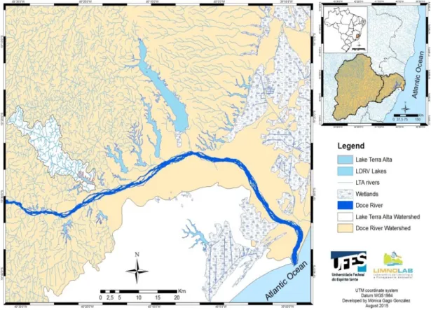
The study area of this study is situated in the southeast coast of Brazil, in the state of Espirito Santo. Being one of the 90 lakes which form the Lower Doce River Valley (LDRV) Lake District, which has an area of 165 km2 (Barroso et al, 2012), Lake Terra Alta (LTA) is a tropical natural lake located in the municipality of Linhares, at the north of the State of Espírito Santo (Figure 3.1).
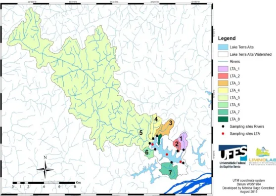
LTA catchment, has an area of 144.7 km2 and is composed by 8 subbasins and 7 tributaries streams (Figure 3.2). The Lake area is 3.9 km2, with a volume of 3,534,8831.06 m3 (0.03 km3). The maximum depth is 22.1 m and its mean depth 9.04 m (Barroso et al, 2012). The lake presents a warm monomictic pattern with thermal stratification on the warm and rainy season, from October to April, and mixing during the dry and cold season, June to September (Venturini, 2015). The retention time based on mean annual discharge of tributary streams is 1.6 years (Barroso et al., 2014), a considerable low value that indicate higher capability of the lake to recover after a disturbance (Ambrosetti, 2002; ILEC 2007)
12
Figure 3.2. Subbasins of LakLTA watershed.
Figure 3.3. Perspective of LTA
13
Based on Köppen climate classes by, the climate on the municipality of Linhares is Aw, a tropical humid climate characterized by a dry winter and maximum rainfall during the summer (Nóbrega et al., 2008)). Considering historical data of 66 years of 13 meteorological stations (Figure 3.5), the regional mean monthly rainfall is higher than 100 mm meanwhile the dry months showed a regional mean monthly rainfall smaller than 50 mm (Barroso et al. 2014). Then, the wet and warm period, comprising the months between October and March, has a mean monthly rainfall of 167,6 mm and a mean temperature of 24,8 ºC . Meanwhile, the dry and mild cold period, comprise the months between April and September and the mean monthly rainfall is 46,1 mm and the mean air temperature 21,9 ºC. According the historical trend, August is consider the driest month and December the wettest month.
Figure 3.5. Regional mean monthly rainfall (1947 to 2013) and monthly rainfall for
2011 and 2013 (Barroso et al., 2014).
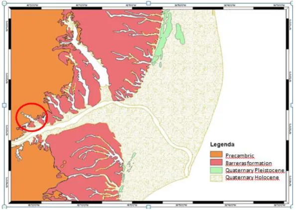
The LDRV Lake District is divided between lakes located in natural dammed alluvial valleys and lakes located on the coastal plain (Martin et al., 1996). According with LTA is inserted in the Barreiras Formation Tertiary Period (Figure 3.6.). The Tertiary plateau is represented by continental deposits divided by subpararel hydrographic network that are drained by small water courses flowing on big valleys of
14
flat bottom silted up with Quaternary sediments. The upper part of its catchment is in the area dominated by Precambrian crystalline rocks drained by a dense dendritic hydrographic net, which presents an uneven relief (Martin et al., 1996).
Figure 3.6. Geomorphological Figure of LDRV. (Modified Limnolab)
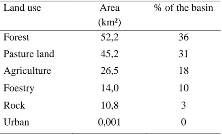
According to the land use of the basin can be consider than the main economic activity is husbandry followed by the agriculture and Eucalyptus forestry. Without considering the natural forest which represents around 36 % of the basin, LTA catchment land use (Table 3.1) is predominantly pastureland, representing approximately a 31 % of the basin. In smaller dimension agriculture with 18% of the basin and a 10% of Eucalyptus forestry. LTA watershed has no urban area or industrial activities.
It is important to mention that the lake host an intensive fish farming facility (Figures 3.7 and 3.8) on floating cages with Tilapia with a production around 15,000 kg of fishes per month.
15
Table 3.1. Land use on LTA watershed.(Barroso et al 2013)
Figure.3.7. Fish farming facility with floating cages.
Figure 3.8. Fish farming facility
Land use Area (km²) % of the basin Forest 52,2 36 Pasture land 45,2 31 Agriculture 26,5 18 Foestry 14,0 10 Rock 10,8 3 Urban 0,001 0
16
In order to provide water for those activities, 33 small irrigation reservoirs were identified in the watershed. Direct lake water withdraw for irrigation, as well as water withdraws from the tributary rivers and fluvial damming represents a pressure for the LTA hydrology, as well as the nutrient inputs from watershed natural loads and anthropogenic activities as agriculture, livestock, forestry and from fish farming which also stress lake trophic state. Those pressures may compromise lake ecosystem services that are provided by water quantity and quality.
17
4. Materials and Methods
4.1 Georeferenced database
A georeferenced database was elaborated with the software ArcGIS 10.1 ESRI® in order to provide the basic information of the hydromorphology of study area as well as the land uses. The coordinate system and datum are UTM and WGS 1984.
A Digital Elevation Model (DEM) of 30 m resolution was used to delimitate LTA subbasins ArcGISwith ArcGIS Hydrology modelling. Once the subbasins were delimitated, the polygons were edited in order to obtain an effective drainage area of the tributary streams, excluding those areas where the water was draining directly to the lake and not through streams.
The river delimitation for the LTA basin and the respective subbasins was done clipping over a hydrography Figure of LDR watershed.
Land use was as well delimited for the entire basin and subbasins in the same way that the previous one based on a Land use Figure of 2010.
4.2 Basin morphometry
Different parameters as watershed area, basin perimeter, basin length, slope, stream number, stream order, stream length, drainage density, stream frecquency, bifurcation ratio, length of overland flow, form factor, circularity ratio, elongation ratio and infiltration number, has been analyzed with the objective to evaluate the watershed morphometry.
All parameters were calculated for the entire LTA basin, as well as for each of the 7 subbasins according to different authors.
- Watershed Area A (km2); Watershed Perimeter P (km ; Watershed length Lb (m)
The total area of the basins, their perimeter and the length between the mouth and the outflow were obtained by ArcGIS (ArcGIS 10.1 ESRI® ) basic geometry tools.
18
-Slope S (%)
Slope is an important parameter to be analyzed in morphometry, because determines the inclination of the terrain (Magesh et al., 2013). Slope is strongly related with runoff, the higher slopes rapid runoff and may result in soil losses. On this study this parameter was calculated in two different ways.
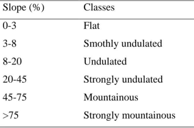
As it was mentioned before, a slope Figure was created with ArcGIS in order to obtain the slope classes in percentage of our study area according to the Brazilian Soil Agency (Table 4.1).
Table 4.1: Slope classification (%) (Embrapa, 1979).
Slope (%) Classes 0-3 Flat 3-8 Smothly undulated 8-20 Undulated 20-45 Strongly undulated 45-75 Mountainous >75 Strongly mountainous
The second way, in order to obtain the mean slope of the basins was calculated following the Romshoo et al., 2012 equation (1) :
S = Dc/L (1)
where,
De is the difference in elevation L is the length of the flow path
- Stream order (U)
The primary step in drainage-basin analysis is to designate stream orders, which is a dimensionless property to hierarchically codify fluvial systems (Horton, 1945). Following the Strahler method (1964) that slightly modifies the Horton´s (1945) which organizes hierarchically the tributaries, stream order was obtained by ArcGIS 10.1 ESRI®. Due to the small size of the basin and number of streams it was possible to do it
19
by hand, selecting the streams and classifying them. The procedure starts from the finger-tip tributaries designated as order 1. If two of those channels connect, they form an order 2 channel segment, which if joins other Order 2 will form an Order 3 tributary and so on, resulting that the highest order stream is the main channel where all discharges of the other streams are leaded. Thus, stream order increase as total number of streams decreases (Magesh et al., 2013). Greater discharge and velocity of the flow are coupled with higher stream order (Romshoo et al., 2012)
- Stream number (Nu)
Horton (1945) defined it as the number of channels that can be found in a stream order, and is proportional to the channel dimension and size of the watershed. In general, on higher stream order there is a decrease on the stream number and lower stream number indicates higher infiltration and permeability (Romshoo et al., 2012; Magesh et al., 2013)
The stream number was obtained after the Stream order classification from ArcGIS 10.1 ESRI®; it was counted on the attribute table as the number of streams belonging to each order.
- Stream length (Lu)
Stream length shows the scale of the components on the drainage network (Strahler 1964). In general, stream length decrease when the stream order increase and the first order presents the maximum total length of stream segments (Magesh et al., 2013).
With the tool, calculate geometry of ArcGIS 10.1 ESRI®, the length of the selected river was calculated.
- Drainage density (Dd)
Dd was calculated according to Hortons (1945) (2) and represents the total stream length Lu per unit of area of the basin A.
Dd = Σ Lu/A (2)
where,
Lu is the stream length A is the area of the watershed
20
Drainage density (Dd) is an important property of a river network being an indicator of the land form (Strahler 1964; Moglen 1998). This geomorphic property is strongly linked with hydrological processes as infiltration or overland flows, and thus, influence their interactions and resulting processes as runoff (Moglen 1998). Different authors as Horton (1945) and Carlston (1963) highlight the importance of permeability and thus infiltration to determine drainage density. The higher drainage density is related with mountainous watersheds with impermeable materials and sparse vegetation that results in lower infiltration capacity and in consequence, a relatively rapid hydrological response to rainfall events. Meanwhile, low drainage density number shows poorly drained basins with slower hydrologic response due to a higher infiltration capacity associated with a good vegetation cover and permeable subsurface materials in low relief areas (Romshoo et al., 2012; Melton 1957).
In general terms the size of drainage units decrease proportionately when drainage density number increase (Strahler 1964).
- Stream frequency (Fs)
The equation (3) from Horton (1945) defines the Stream frequency (Fs), where Nu is the number of stream segments and A is the basin area. This parameter is related to permeability, infiltration capacity and relief of watersheds (Montgomery and Dietrich 1989; Romshoo et al., 2012).
Fs = Σ Nu/A (3)
where,
Nu is the number of stream segments A is the area of the watershed
-Bifurcation ratio (Rb)
According to Schumm (1956) equation (4) , the Bifurcation ratio depends on the stream number, defining a ratio between the stream number of an order (Nu) and the stream number of the next higher stream order (Nu+1). This parameter contribute to the understanding of the branching pattern of a drainage network (Magesh et al., 2013), being an useful number to define the form of the drainage basin, specially due to its stability because in general is representative in different environments or regions with the exception of areas or high geologic controls (Strahler 1964).
21
Rb = (Nu) / (Nu + 1) (4)
where,
Nu is the number of stream segments
This parameter indicates the vulnerability of the basin for flooding if it presents a high value (Romshoo et al., 2012). The mean bifurcation ratio ranges between 3 and 5 if there is not strong influence of the geological characteristics of the drainage network, and low values indicates poor structural disturbances and higher permeability of the terrain (Magesh et al., 2013) meanwhile higher values are related with well-dissected, hilly drainage basins (Horton 1945).
-Length of overland flow (Lg)
The length of overland flow determine the distance that the rainwater need to reach a definite stream channel and can be calculated with the equation of Horton (1945) (5) and in most cases it is approximately the half to reciprocal of the Drainage density. Horton describes this parameter as one of the most important variables that influence the drainage basin development in hydrologic and physiographic terms being an important variable on which runoff and flood processes depend (Zavoianu 1985; Romshoo et al., 2012).
Lg = 1/(Dd*2) (5)
where,
Dd is the drainage density
Higher values indicate higher distances and lower values shorter distances before to reach the stream channels (Magesh et al., 2013).
-Form factor (Rf )
The Form Factor is one of the most relevant shape related parameters in the morphology. The equation proposed by Horton (1945) (6) define the Form factor, where its related the area of the basin (A) and its length, represented by Lb, the farthest distance from watershed ridge to outlet.
22
Rf = (A) / (Lb + 1)² (6)
where,
Lb is the farthest distance from watershed ridge to outlet or watershed length (m) A is the area of the watershed
Form factor values closer to 1.0 represent circular basins and as longer and narrower the basin is, its form factor value is decreasing due to their higher lengths (Magesh et al., 2013).
-Elongation ratio (Re)
This parameter measure the shape of the basin of the river linking the diameter of circle with the area and the maximum length of the basin (Magesh et al., 2013) and is calculated by the Schumm (1956) equation (7).
Re = (2/π) √ ( A / Lb) ² (7)
where,
Lb is the farthest distance from watershed ridge to outlet or watershed length (m) A is the area of the watershed
More circular basins seems to be more efficient in the runoff discharge due to a lower concentration time, they are representatives of lower reliefs and their Re values are closer to 1.0. Meanwhile elongated basins with higher relief are closer 0.6 values (Magesh et al., 2013). The results of the elongation ratio should be similar to the form factor (Strahler 1964).
-Circularity ratio (Rc)
Circularity ratio influences the hydrological response of the watersheds as basin-shaped (Romshoo et al., 2012). This shape related parameter was defined by Miller (1953) as a ratio of the area of the basin and the area of a circle. Is an indicator of the dendritic stage of a watershed and the stage of the life cycle of the tributary basins (Magesh et al., 2013). This parameter was calculated with the equation (8)
23
where,
A is the area of the watershed P is the perimeter of the watershed
-Infiltration number (If )
To describe the infiltration capacity of the basin the equation proposed by Romshoo (2012) was used (9). This number is inversely proportional to the infiltration capacity (Romshoo et al., 2012)
If = Dd× Fs (9)
where,
Dd is the drainage density Fs is the stream frequency
4.3 In situ discharge measurements
Stream discharge measurements were taken between 2012 and 2013 in 7 sampling events: 4 during dry season and 3 during wet season for the seven LTA. Stream discharge measurements (m3/s) were taken on the outfall of all 7 LTA tributary streams with a SonTek FlowTracker Acoustic Doppler Velocimeter – ADV .
4.4 Hydrological modeling
This section presents a hydrological modeling based on conversion of rainfall on river discharge, discounting potential evapotranspiration according to Molisani et al. (2006) and Molisani et al., (2007). Rainfall data are based on regional historical records of rainfall (i.e., 30 years) of 21 meteorological stations. Mean annual rainfall and mean values for the dry and wet months, August and December, respectively, were interpolated (Spline with 0.2 weight on 6 neighbors) in a GIS environment for the LDRV. The continuous surface model (i.e., raster file) of regional rainfall was than clipped to the boundaries of LTA watershed. Evapotranspiration rates based on air temperature at every 100 m elevation were adiabatically corrected.
24
Acording to Kjerfve (1990), the equation 10 show that discharge is directly dependent on precipitation, area, and the runoff ratio (∆f /r)
Q = ∫∫ r * (∆f / r ) *dA (10)
where:
Q is the discharge (m3/s) r is the precipitation (mm/y)
A is the area of the watershed (km2) ∆f /r is the runoff ratio
The runoff ratio is in turn dependent of the potential evotranporation (E0 ) and
precipitation (r), it can be calculated with the equation of Schreiber (1904) (11) and represents the fraction of precipitation, which drains into the rivers as a runoff (Molisani 2006).
∆f / r = e –E0/r (11) where:
∆f /r is the runoff ratio
E0 is the potential evotranporation (cm/year)
To calculate the runnoff ratio is necessary the previous calculation of the potential evotranporation (E0 cm/year) (12) , which depends on the solar radiation intensity,
which is turns means that depends on the absolute air temperature. Is described by Holland (2001) (Molisani 2006).
E0 = 1.0×10⁹ × e−4620 /T (12)
where:
E0 is the potential evotranporation (cm/year)
T is the absolute air temperature expressed in Kelvin (K)
To sum it all up now that the process is described, to calculate the discharge we need the precipitation which has been calculated previously with the interpolation method and air temperature. On this case temperature measurements were not available, so a reference temperature value from the adjacent area is necessary and its correction adiabatically by
25
-0,97ºC per 100m of elevation increase (List, 1966). The rainfall data was converted to obtain the precipitation rate.
The obtained discharges were transformed in Effective Discharge (13) multiplying by a time unit and divided by the area of the basin. In case of annual mean was multiplied by 365 days obtaining and Effective discharge in m³/km²/year meanwhile for the dry and wet month was multiplied by 31 days obtaining m³/km²/month because the wet and dry months have 31 days each. Through this transformation the results can be compared between the basins because the influence of the total area is excluded.
Qe = Q*time / A (13) where:
Qe is the effective discharge Q is the direct discharge A is the area of the watershed
On case of the In situ discharge measurements, the transformation to Effective discharge follows the same procedure, but for wet/dry month was necessary to select them from the sampling dates. According to Figure 3.5 and the sampling dates for the wet month was consider November 2012 and August 2013 for the dry. Then, was necessary consider that August has 31 days but November only 30 when the calculations of effective discharge are done.
4.6 Hydrochemistry analysis
N and P flows were based on concentrations of stream water samples, taken between 2012 and 2013 on 7 sampling events, three during the dry season (< 50mm/yr) and four on wet season (> 100mm/yr), at the outfall of the 7 LTA tributary streams. For total N and P, samples were frozen without filtration, whereas for dissolved inorganic nitrogen (DIN) and phosphorus (PID) samples were filtered (Whatmann fiber glass 934AH) in the field right after sampling and stored on 100 mL polypropylene flasks. All samples were frozen immediately. The analysis was carried out at UFES’ LimnoLab located in Goiabeiras campus through spectrophotometry (UV/VIS).
26
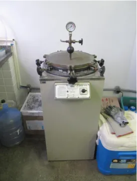
Total fractions of N and P were digested (Figure 4.1.) on persulfate solution according to Valderrama (1981), a method which shows good reliability and allow the storage of the sample till the analysis. The simultaneous oxidation depends on the difference of pH during the digestion due to a boric acid-sodium hydroxide system, starting the reaction in an alkaline medium, which allows the oxidation of the nitrogen, and progressively decreasing the pH till obtain an acidic environment for the phosphorous oxidation.
Figure 4.1 Autoclave of Limnolab (UFES)
PT was analyzed after the digestion through a colorimetric method according to Carmouze (1994). The absorbances were measured in a spectrophotometer on four 1 cm glass cells at a wave length of 885 nm. The absorbances obtained were corrected with the value of the blanks and applied to the regression curve to obtain the final concentration.
For nitrogen were just analyzed nitrite (NO2-) and nitrate (NO3-) because it was not
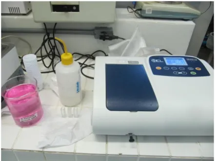
possible the quantification of ammonia and organic nitrogen, therefore is important to consider that when in the present study we refer to TN we are only considering nitrites and nitrates. Nitrite was determined according to Grasshoff et al. (1999) method, where nitrite is quantified by spectrophotometry (Figure 4.2) of the azo dye resulting from the reaction of nitrite with an aromatic amine which leads to the formation of a diazonium compound which couple with a second amine. The absorbances obtained were corrected with the value of the blanks and applied to a regression curve to obtain the final
27
concentration of nitrite. This methodology was followed although there are no saltwater samples, due to the analytical limitations.
For nitrate determination was used the Cd column method (Figure 4.3) according to Carmouze (1994) which consists in the reduction of nitrate to nitrite. The yield of the reduction is very sensitive and highly dependent on the metal used (i.e., Cd) in the reduction and the activity of the metals surface as well as pH. If the previous variables are not the appropriated, it will result in a partial reduction, which results in too low nitrate values (Grasshoff et al.1999). The resulting nitrite was quantified by the method described above.
Figure 4.2. Spectophotometry. Limnolab. (UFES)
28
N and P flows were computed, based on the concept of Wagner (2009) of point source load computation according to the equation (14),
Cday = C*Q*86400 (14)
Where,
Cday is load or flow (g/day)
C is the concentration (g/m3)
Q is the instantaneous discharge (m3/s) 86,400 seconds per day.
This equation was modified (15) to obtain the load or flow of nutrients on yearly base for the annual mean (nutrient/year) or monthly base for wet and dry month (nutrient/month). The concentration of nutrients (C) was multiplied by the specific discharge for each measurement of each subbasin (Q) to obtain the average of the subbasin, which finally was multiplied by 86400 seconds/day and by 365 days on case the annual mean and 31 days for the wet and dry month, being all the process consequently adapted with the convenient unit conversion to obtain kg/year or kg/month.
Tnutrient/year = C*Q*86400*365 (15)
Tnutrient/month = C*Q*86400*31 Where,
Tnutrient is the total load of TN or TP C is the concentration (g/m3)
Q is the instantaneous discharge (m3/s)
As well as for the water discharge, the nutrient load was converted into TN and TP effective discharge (TNED and TPED) (16) dividing the load by the area of each subbasin (A). This is useful in order to standardize the flows regarding the area of subbasins.
29
Where,
Tnutrient is the total load of TN or TP
TNED /TPED are the TN and TP effective discharges C is the concentration (g/m3)
Q is the instantaneous discharge (m3/s)
4.7 Statistical analysis:
In order to whether know the interaction between water quality, hydromorphological variables and land use can be recovered as statistically significant covariance patterns was used the Principal component analysis (PCA).
-Multivariate analysis, Principal Component Analysis (PCA).
The multivariate analysis consists in the representation of scattered variables and cases in a multidimensional diagram with as many axes as descriptors in the study. Nevertheless, as is not possible to represent more than two or three dimensions on paper, those diagrams are represented onto bivariate graphs whose axes are of special interest, specifically chosen to represent the variability of the data set in a space of reduced dimensionality (Legendre and Legendre, 1998).
Principal component analysis PCA is one of those methods of ordination in reduced space which allows the identification of the most important components that explain nearly all of the variances of the system, providing a shortened description with few significant indices that reflect the most relevant processes (Petersen et al., 2001; Ouyang, 2005). The PCA, project those representative features into two-dimensional axes independent between them, and even reducing the data complexity, the relationships between the variables are mainly maintained (Janžekovič and Novak, 2012). The number of the components is the same than the variables, nevertheless a component is formed by all the variables (Ouyang, 2005). Legendre and Legendre (1998) argue that the number of observations cannot be smaller than the number of descriptors to obtain a statistical valid estimation of the dispersion matrix, nevertheless other studies have shown that regardless the number of observations and descriptors PCA could be applied (Ouyang, 2005).
30
On this study the PCA analysis was runned with the Multi Variate Statistical Package software MVSP 3.2, where the data were log10 transformed and centered and only axis 1 and 2 reported.
-Cluster analysis
This analysis consists on the partition of our set of objects or descriptors in two or more subsets, the clusters, through pre-established rules of agglomeration or division (Legendre and Legendre, 1998).
The subbasins of LTA catchment are the descriptors that we want organize, for this proposal the method of cluster selected is the hierarchically where according to Legendre and Legendre (1998) the two more similar descriptors are cluster and then the rest of the descriptors clump into groups which at the same time are aggregate to other groups as the similarities diminish. The easiest way of interpretation of this analysis is graphical representation, a Dendogram. The cluster analysis was run with the MultiVariate Statistical Package software MVSP 3.2, where the data were log10 transformed.
31
5. Results
5.1 Georeferenced database
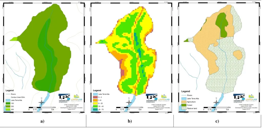
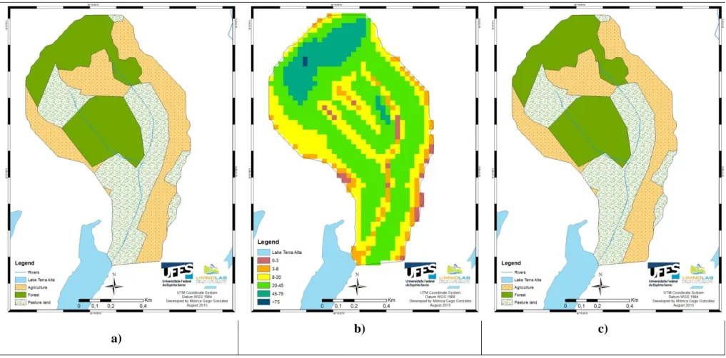
The resulting Figures of the georeferenced data base are presented by subbasin grouped in sets of three, where the first represents the altimetry classes each 100 m elevation, the second one represents the land use and the third one, the slope according the Embrapa 1979 soil classification. B1 is represented on Figure 5.1. , B2 on Figure 5.2. , B3 on Figure 5.3. , B4 on Figure 5.4. , B5 on Figure 5.5. , B6 on Figure 5.6. and B7 on Figure 5.7.
32
a) b) c)
33
a) b) c)
Figure 5.2. Subbasin B2 elevation (a), slope (b) and land use/land cover (c).
34
a) b) c)
35
a) b) c)
Figure 5.4. Subbasin B4 elevation (a), slope (b) and land use/land cover (c).
36
a)
b)
c)
37
a) b) c)
Figure 5.6. Subbasin B6 elevation (a), slope (b) and land use/land cover (c).
38
a) b) c)
Figure 5.7. Subbasin B7 elevation (a), slope (b) and land use/land cover (c).
39
5.2 Basin morphometry
On this section the all the obtained numerical results of the morphological parameters are presented on Table 5.1.
-Watershed Area A (km2)
The entire watershed of LTA has an area of 144 km². B5 is the biggest subbasin with an area of 122.5 km². The other subbasins have much smaller values. being presented in decreasing order B7 (3.32 km²). B4 (2.88 km²). B3 (2.83km²). B1 (1.89 km²). B6 (1.39 km²) and the smaller one. B2 (0.98 km²)
-Watershed Perimeter P(km)
The perimeter follow the same trend as the area, ranging in decreasing order from B5 followed by B7, B4, B3, B1, B6, till B2 being their respective values 87.41km , 8.94 km, 8.48 km, 8.22km , 6.66km, 5.54km, 4.31km.
-Watershed length Lb (km)
On the watershed length we can observe some variations in the order compared with area a perimeter due to the shape of the basins. From the entire basin of LTA (27.71 km) the subbasin B5 (22.45km) still being the one with higher value, nevertheless B7 is not anymore the next higher value, ranging now from B4 (3.09km), B3 (2.92km), B1 (2.24 km), B7 (2.04km), B6 (1.59km) , till B2 (1.53km) which still maintain the smallest values.
-Slope S (%)
According theSilva et al., 2010 equation (1), the values of the slope are as follow: LTA 34.06%, B1 22.92%, B2 34.92%, B3 32.66%, B4 38.07%, B5 35.93%, B6 23.77%, B7 4.91%. Where B4 presents the highest slope followed by B5, B2, B3, B6, B1 and finally B7. The subbasin is consider strongly undulated according the Embrapa (1979) (Table) classification, and its subbasins as well, with the exception of the B7 which presents a much smaller value and is considered smoothly undulated.
For a more detailed vision of the slope distribution the representation of the slope for each subbasin in classes according to Embrapa(1979) soil classification was exposed on
40
the previous section 3.1 results of georeferenced database, concretely on Figures 5.1., 5.2., 5.3., 5.4, 5.5., 5.6., and 5.7.
- Stream order (U)
LTA have 4 stream orders as we can see on the Figure 5.8. , but we can only find those 4 orders in the subbasin B5. Meanwhile B2, B3, B4, B6 and B7 presents 2 orders and only B1 have 1 order.