Spatial Variability of Soil Fauna Under Different Land Use and Managements

(1)

* Corresponding author: E-mail: gleciosiqueira@hotmail.com

Received: April 13, 2017 Approved: November 5, 2017 How to cite: Silva RA, Siqueira GM, Costa MKL, Guedes Filho O, Silva EFF. Spatial variability of soil fauna under different land use and managements. Rev Bras Cienc Solo. 2018;42:e0170121.

https://doi.org/10.1590/18069657rbcs20170121

Copyright: This is an open-access article distributed under the terms of the Creative Commons Attribution License, which permits unrestricted use, distribution, and reproduction in any medium, provided that the original author and source are credited.

Spatial Variability of Soil Fauna Under

Different Land Use and Managements

Raimunda Alves Silva(1)

, Glécio Machado Siqueira(1)*

, Mayanna Karlla Lima Costa(1) , Osvaldo Guedes Filho(2) _{and Ênio Farias de França e Silva}(3)

(1)

Universidade Federal do Maranhão, Departamento de Geociências, São Luís, Maranhão, Brasil. (2)

Universidade Federal do Paraná, Campus Avançado Jandaia do Sul, Jandaia do Sul, Paraná, Brasil. (3)

Universidade Federal Rural de Pernambuco, Departamento de Engenharia Agrícola, Recife, Pernambuco, Brasil.

ABSTRACT: Geostatistics allows the evaluation of the distribution pattern of data with

high spatial variability in agricultural systems. This study aimed to evaluate the spatial variability of biological diversity indices of soil fauna under different land (agriculture and forest). Samples were collected in seven areas (millet, soybean, corn, eucalyptus, pasture crops, and preserved and disturbed Cerrado), in Maranhão state, Brazil. The soil fauna was caught trapped in pitfall traps, installed 3 m away from each other. In each area, 130 traps were maintained for seven days. After this period, they were removed and their content transferred to bottles and taken to the laboratory, where the insects were screened and identified at the level of orders and families. Eight indices were calculated, namely: individuals trap-1 _day-1_{, Jackknife richness estimator, the Simpson,}

McIntosh, Shannon, and total diversity, and Simpson dominance, and Pielou equitability indices. The spatial variability was derived from the semivariograms fitted to Gaussian, spherical, and exponential geostatistical models. Statistical analysis showed medium values of the coefficient of variation for millet, except for the indices individuals trap-1_day-1

and McIntosh diversity, which were considered high. The values of the correlation matrix were negative for some indices, suggesting an inverse relationship. For millet, corn, eucalyptus, disturbed Cerrado, and pasture areas, the Shannon diversity index exhibited a pure nugget effect. For the areas of millet, corn, disturbed Cerrado and pasture, the total diversity index was adjusted to the Gaussian model. The degree of spatial dependence was considered high for the individuals trap-1_day-1_{and Pielou equitability indices for millet.}

Only for soybean and pasture similarity in the scaled semivariograms was observed for the spatial variability of the indices, indicating similarity of performance. Soil management and land use affect the patterns of soil fauna abundance, richness, and diversity. The presence of groups such as Araneae, Diplura, and Poduromorpha are related to ecological equilibrium, quality, and sustainability of the agricultural systems studied.

Keywords: soil biodiversity, soil properties, geostatistics.

(2)

INTRODUCTION

The use of geostatistics in analysis of soil properties variability has increased significantly over the last decades. In a given area, geostatistical techniques can identify properties that are treated as homogeneous but would need a differentiated management (Ribeiro et al., 2016). Moreover, by these techniques, soil properties can be understood, modelled, and mapped to identify specific management zones and reduce the effects of soil variability on crop yields (Siqueira et al., 2009; Chiba et al., 2010; Montanari et al., 2010; Carvalho et al., 2014; Zonta et al., 2014; Aquino et al., 2015; Montanari et al., 2015; Siqueira et al., 2015a, 2017).

Soil variability occurs due to the interaction of formation factors, climate, temperature, and management (Bonnin et al., 2010; Siqueira et al., 2017), which directly affects agricultural productivity (Basso et al., 2011). The different planting systems can alter the soil quality, due to constant fertilization and liming, resulting in changes in the physical, chemical, and biological soil properties (Baretta et al., 2003; Carvalho et al., 2014).

The no-tillage system plays an important role in the conservation and maintenance of soil biota (Crusciol et al., 2010; Pedroso et al., 2016), due to the reduced soil disturbance, residue accumulation (Cunha et al., 2011), and crop rotation (Paul et al., 2013), which stabilize habitats and food supply (Bottega et al., 2013). In terms of soil benefits, the no-tillage system minimizes evaporation and erosion and can increase soil water infiltration and microbial activity rates, favoring nutrient incorporation in the soil and improving the physical, chemical, and biological quality.

Several studies have addressed soil fauna as a soil quality promoter (Vasconcellos et al., 2013; Rousseau et al., 2014; Moura et al., 2015). The soil biota comprises organisms of the most diverse sizes, which have been studied to evaluate changes in the environments (Rousseau et al., 2014). In general, changes in group abundance, diversity, and composition reflect disturbances of the ecosystem (Domínguez et al., 2014). Agricultural practices cause numerous changes in the composition and distribution of soil biota, directly affecting soil processes such as nutrient cycling, organic matter decomposition, porosity, and water infiltration (Vries et al., 2013; Wagg et al., 2014; Siqueira et al., 2016).

Since the distribution of soil properties in the areas is irregular, an evaluation of the spatial distribution of the physical, chemical, and biological properties is essential to improve decision making with regard to crop management and production. The objective was to evaluate the spatial variability of biological diversity indices of the soil fauna under different land uses (millet, corn, soybean, eucalyptus, and pasture) and soil cover (preserved Cerrado and disturbed Cerrado).

MATERIALS AND METHODS

The study was carried out on the FazendaUnha de Gato, municipality of Mata Roma, Maranhão, Brazil (3° 70’ 80.88” S and 43° 18’ 71.27” W). According to the Köppen classification system, the regional climate is humid tropical, with mean annual temperatures from 27 to 30 °C, a dry season from June to November, and a rainy season from December to May. Rainfall ranges from 1,400 to 1,600 mm and annual evapotranspiration is 1,144 mm (data measured at the meteorological station in the experimental area). The soil of the region is an Oxisol (Soil Survey Staff, 1999).

(3)

formaldehyde (200 mL) for the preservation of organisms, according to the methodology described by Aquino et al. (2001) and Siqueira et al. (2014).

The traps were installed at a distance of 3.0 m from each other and left in the field for seven days. After this period, all contents were preserved in 70 % alcohol and screened. The groups were separated in large groups and family based on identification keys, according to Lawrence (1994). Subsequently, the biodiversity indices were generated, based on the identification of groups.

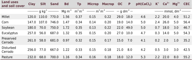
Soil samples were collected in each transect (0.00-0.20 m layer) to evaluate the relationships between soil chemical (organic carbon, P, pH, K, Ca, Mg, and CEC) and physical properties (sand, silt, clay, bulk density, total porosity, macroporosity, and microporosity) and the soil macrofauna in the study areas. The mean values of the soil chemical and physical properties in the areas are listed in table 1.

Table 1. Soil physical and chemical properties in the study areas

Land uses

and soil cover Clay Silt Sand Bd Tp Microp Macrop OC P pH(CaCl2) K +

Ca2+ Mg2+ CEC

g kg-1

Mg m-3

m3

m-3

m3

m-3

g dm-3

mmolc dm-3

Millet 120.0 110.0 770.0 1.56 0.37 0.15 0.22 29.0 18.0 4.6 2.2 20.0 4.0 51.2 Corn 147.0 107.0 746.0 1.47 0.34 0.14 0.20 19.0 14.0 5.0 2.4 26.0 5.0 56.4 Soybean 180.0 70.0 750.0 1.72 0.35 0.13 0.22 22.0 49.0 5.0 0.7 18.0 3.0 46.7 Eucalyptus 257.0 56.0 687.0 1.32 0.35 0.15 0.20 27.0 10.0 4.7 0.3 14.0 5.0 54.3 Preserved

Cerrado 261.0 58.0 681.0 0.97 0.32 0.15 0.17 15.0 7.0 4.1 0.2 2.0 1.0 35.2 Disturbed

Cerrado 256.0 77.0 667.0 1.22 0.33 0.15 0.18 21.0 8.0 4.2 0.5 3.0 3.0 42.5 Pasture 232.0 68.0 700.0 1.16 0.34 0.16 0.18 18.0 12.0 5.3 2.2 22.0 8.0 55.2

Bd = bulk density; Tp = total porosity; Microp = microporosity; Macrop = Macroporosity; OC = organic carbon; P = phosphorus; K = potassium; Ca = calcium; Mg = magnesium; CEC = cationic exchange capacity. The properties were determined according to the methodology described by Camargo et al. (2009).

Figure 1. Location of study areas. 1 and 2 = soybean and millet; 3 = corn; 4 = eucalyptus; 5 = pasture; 6 = preserved Cerrado; and 7 = disturbed Cerrado.

700000 701000 702000 703000

9589500

9590000 N

S E W

9590500 9591000 9591500 9592000 9592500

99 101 103 105 1) Soybean – 90.35 ha

2) Millet – 90.35 ha 3) Corn – 71.51 ha 4) Eucalyptus – 5.71 ha 5) Pasture – 1.72 ha

6) Preserved Cerrado – 19.35 ha 7) Anthropic Cerrado – 49.13 ha

1 and 2 6

3

4

5

(4)

Diversity indices

To determine the biodiversity indices, software DivEs (Rodrigues, 2015) was used. The index individuals trap-1 day-1 was calculated from the number of individuals collected per trap and divided by the number of days in which the trap remained in the field, in this case, seven days.

The first-order Jackknife richness index estimates the richness of a community. It is defined as a function of the number of species that occur in only one sample, termed single species. Thus, the larger the number of species in a single sample, the higher the estimate for the total number of species in the community (Equation 1):

ED= Sobs + S1

ƒ - 1

( )

ƒ _{Eq. 1}

in which: Ed is Jackknife richness index; Sobs is the number of observed species; S1 the

number of species present in a single cluster; and f the number of samples.

Simpson’s diversity index is used to quantify infinite communities, that is, in cases which the total number of individuals in a sample is different from the total number of individuals in the community (Equation 2). This index is appropriate to estimate diversity when sampling involves the counting of individuals:

Ds= Σ

ni (ni - 1)

N (N - 1) _{Eq. 2}

in which: Ds is Simpson diversity index; ni is the number of individuals of species i in the sample; N is the total number of individuals in the sample.

The McIntosh diversity index is a more complex index because, apart from considering the total number of individuals, it takes square root of the sum of the number of individuals of each species into account (Equations 3 and 4):

D = _{N -}N - U_√N

Eq. 3

U= √Σn

i = 1 n2i Eq. 4

in which: D is the McIntosh diversity index; N is the total number of individuals in the sample(s); U the square root of the sum of the squared number of individuals per species.

The Shannon-Wiener diversity index is the most commonly used index in community studies. Shannon values range from 0 to 3.5, rarely exceeding 4.5 (Magurran, 1988). The index will be zero if a sample contains only one species and reaches the maximum value when all species of a sample have the same number of individuals (Equation 5):

H'= Σn

i = 1 pi × log10 pi Eq. 5

in which: H’ is Shannon-Wiener diversity index; ni is the number of individuals of species i in the sample; N is the total number of individuals in the sample; log10 is the logarithm

(base 10).

The diversity of a region, i.e., total diversity, can be estimated as a function of the species variation (Equation 6):

TD= Σn

i = 1wi [pi (1 - pi)] Eq. 6

(5)

Simpson’s dominance is determined by the Simpson diversity index (Equation 7):

D_S= 1

-N (-N - 1 )

Σi n n_i × (n - 1)

( )

Eq. 7

in which: Ds is the Simpson dominance; ni is the number of individuals of each species;

and N the number of individuals.

The Pielou equitability indicates the distribution of individuals among species and is proportional to diversity and inversely proportional to dominance. Equitability compares the Shannon-Wiener diversity with the observed species distribution that maximizes diversity (Equation 8):

U= H'

log₁₀ S _{Eq. 8}

in which: U is the Pielou equitability; H’ is the Shannon-Wiener index; S is the number of groups present in each area; and log10 is the logarithm to base 10.

Geostatistical and statistical analysis

Descriptive statistics were determined using the statistical program R (R Development Core Team, 2009), where the values of maximum, minimum, mean, standard deviation, coefficient of variation (CV), skewness, kurtosis, and normality were calculated by the Kolmogorov-Smirnov test at 0.01 % probability. The linear correlation matrix of Pearson was calculated for all soil properties, according to the classification of Santos (2007), considering r values up to 0.5 as low and above 0.5 as high.

Multivariate statistics were applied to data of physical, chemical, and biological soil properties, using the factorial exploration technique to identify relationships between them. For the factorial analysis, collinearity-free data were selected and standardized (null mean and unit variance). The factors were extracted by principal component analysis calculated from the correlation matrix between variables. The properties with factor loadings above 0.7 in absolute value were selected (Jeffers, 1978). Multivariate analysis was carried out using software Statistica 7.0.

The spatial variability was analyzed through the construction of a semivariogram γ (h) of a spatially distributed variable, as proposed by Vieira (2000) (Equation 9).

γ (h)= 1

2N (h) Σi = 1 N(h)

[z(xi) - z(xi + h)]2

Eq. 9

in which: γ(h) is the spatial variability; N(h) is the number of observations separated by distance h. All semivariograms were fitted to a mathematical model according to the range (a), sill (C0+C1), and nugget effect parameters (C0).

The intrinsic hypothesis of geostatistics was considered, which requires no finite variance, Var(z) butonly stationarity of the mean and second-order stationarity of the differences

[(z (x) -z (x + h)] (Journel and Huijbregts, 1978). The semivariograms were scaled as described by Vieira et al. (1997) (Equation 10).

γsc₍_h₎₌ γ(h)

Var(z) _{Eq. 10}

in which: ysc_(h)_{is the scaled semivariogram;}_y(h)_{is the original semivariogram, and} Var(h) is the data variance.

(6)

The spatial dependence ratio was calculated according to the equation 11.

RD = C0 C₀ + C₁

( )

× 100

Eq. 11

in which: RD is the ratio of dependency; C0 is the nugget effect; C0+C1isthe sill.

And classified as proposed by Cambardella et al. (1994), in strong (0-25 %); moderate (25-75 %); and weak (75-100 %).

RESULTS AND DISCUSSION

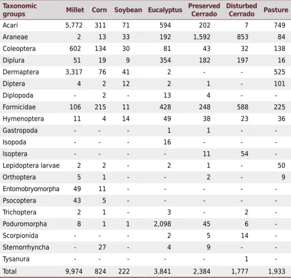
The sampled arthropods were classified into 20 taxonomic orders and one family. The representativeness was highest in the millet area, with 9,974 individuals, followed by eucalypt with 3,841 individuals. The lowest abundance was in the area with soybean (222 individuals) (Table 2).

Poduromorpha tends to be better represented in areas with organic residues in the soil, where it is also captured in greater abundance (Baretta et al., 2003; Rafael et al., 2012). These organisms are used as bioindicators of soil quality and environmental disturbances, being key organisms for the detection of degraded areas. In the eucalyptus area, although there is a thick layer of organic matter, the contribution of the class Poduromorpha is relevant, because they are important as consumers, for nutrient cycling, and responsible for soil enrichment.

Table 2. Composition of the soil fauna under different use and management in the Cerrado Biome

Taxonomic

groups Millet Corn Soybean Eucalyptus

Preserved Cerrado

Disturbed

Cerrado Pasture

Acari 5,772 311 71 594 202 7 749 Araneae 2 13 33 192 1,592 853 84 Coleoptera 602 134 30 81 43 32 138 Diplura 51 19 9 354 182 197 16 Dermaptera 3,317 76 41 2 - - 525 Diptera 4 2 12 2 1 - 101 Diplopoda - 2 - 13 4 - -Formicidae 106 215 11 428 248 588 225 Hymenoptera 11 4 14 49 38 23 36 Gastropoda - - - 1 1 - -Isopoda - - - 16 - - -Isoptera - - - - 11 54 -Lepidoptera larvae 2 2 - 2 1 - 50 Orthoptera 5 1 - - 2 - 9 Entomobryomorpha 49 11 - - - - -Psocoptera 43 5 - - - - -Trichoptera 2 1 - 3 - 2 -Poduromorpha 8 1 1 2,098 45 6 -Scorpionida - - - 2 5 14 -Sternorrhyncha - 27 - 4 9 - -Tysanura - - - 1 -Total 9,974 824 222 3,841 2,384 1,777 1,933

(7)

The correlation matrix between soil fauna taxa and soil chemical and physical properties was null (<0.05) (data not shown). In a study on the spatial relationship between macrofauna and soil properties, Gholami et al. (2016) stated that this correlation is difficult to describe. The reasons are the sensitivity and dynamics of the soil macrofauna, depending on soil use and management, once these organisms respond to the slightest environment alterations.

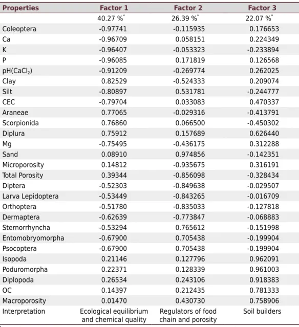
Multivariate analysis grouped the data in three classes, which together explain 88.75 % of the original data (Table 3). The factors 1, 2, and 3 explained 40.27, 26.39, and 22.07 %, respectively, of the total variation.

Factor 1 describes the ecological equilibrium and soil chemical quality in the studied environment. It involves the groups of predators, recyclers of organic matter and groups involved in soil decomposition processes such as Araneae (0.77065), Scorpionida (0.76860), Diplura (0.75912), and Coleoptera (-0.97741). This factor had a strong negative correlation with the following soil properties: silt (-0.80897), P (-0.96085), pH (-0.91209), K (-0.96407), Ca (-0.96709), Mg (-0.75495), and CEC (-0.79704).

Table 3. Factor analysis with the first three factors and factorial charge that represent the correlation

coefficients between soil properties and each factor

Properties Factor 1 Factor 2 Factor 3

40.27 %*

26.39 %*

22.07 %*

Coleoptera -0.97741 -0.115935 0.176653 Ca -0.96709 0.058151 0.224349 K -0.96407 -0.053323 -0.233894 P -0.96085 0.171819 0.126568 pH(CaCl2) -0.91209 -0.269774 0.262025

Clay 0.82529 -0.524333 0.209074 Silt -0.80897 0.531781 -0.244777 CEC -0.79704 0.033083 0.470337 Araneae 0.77065 -0.029316 -0.413791 Scorpionida 0.76860 0.066500 -0.450302 Diplura 0.75912 0.157689 0.626440 Mg -0.75495 -0.436175 0.312288 Sand 0.08910 0.974856 -0.142351 Microporosity 0.14812 -0.935675 0.316191 Total Porosity 0.39344 -0.856098 -0.328434 Diptera -0.52303 -0.849638 -0.029507 Larva Lepidoptera -0.53449 -0.843265 -0.016709 Orthoptera -0.51780 -0.835033 -0.127818 Dermaptera -0.62639 -0.773847 -0.068883 Sternorrhyncha -0.53294 0.765612 -0.151998 Entomobryomorpha -0.67900 0.705438 -0.199904 Psocoptera -0.67900 0.705438 -0.199904 Isopoda 0.21146 0.127796 0.962091 Poduromorpha 0.22371 0.128339 0.961003 Diplopoda 0.26534 0.243106 0.918383 OC 0.14397 0.212435 0.781333 Macroporosity 0.01470 0.430730 0.758906 Interpretation Ecological equilibrium

and chemical quality

Regulators of food chain and porosity

Soil builders

*

(8)

Factor 2 grouped the food chain regulators and soil porosity, with a strong positive correlation with the groups Entomobryomorpha (0.705438), Psocoptera (0.705438), and Sternorrhyncha (0.765612). This indicates that these groups are related to macroporosity (-0.935675), sand (0.974856), and total porosity (-0.856098), which demonstrates their contribution to organic matter decomposition and soil structuring.

Factor 3 grouped the soil properties called soil builders, with a strong positive correlation to all properties. The groups Diplopoda (0.918383), Isopoda (0.962091), and Poduromorpha (0.961003) are related to organic matter input and relevant in nutrient recycling and soil enrichment (Bedano et al., 2016). The presence of the groups of soil builders and organic matter decomposers contributed positively to the sustainability of the productivity of agricultural systems. In this way, the soil fauna is the transforming agent of chemical, physical, and biological properties of the soil (Correia, 2002; Blanchart et al., 2006; Bottinelli et al., 2015; Franco et al., 2016).

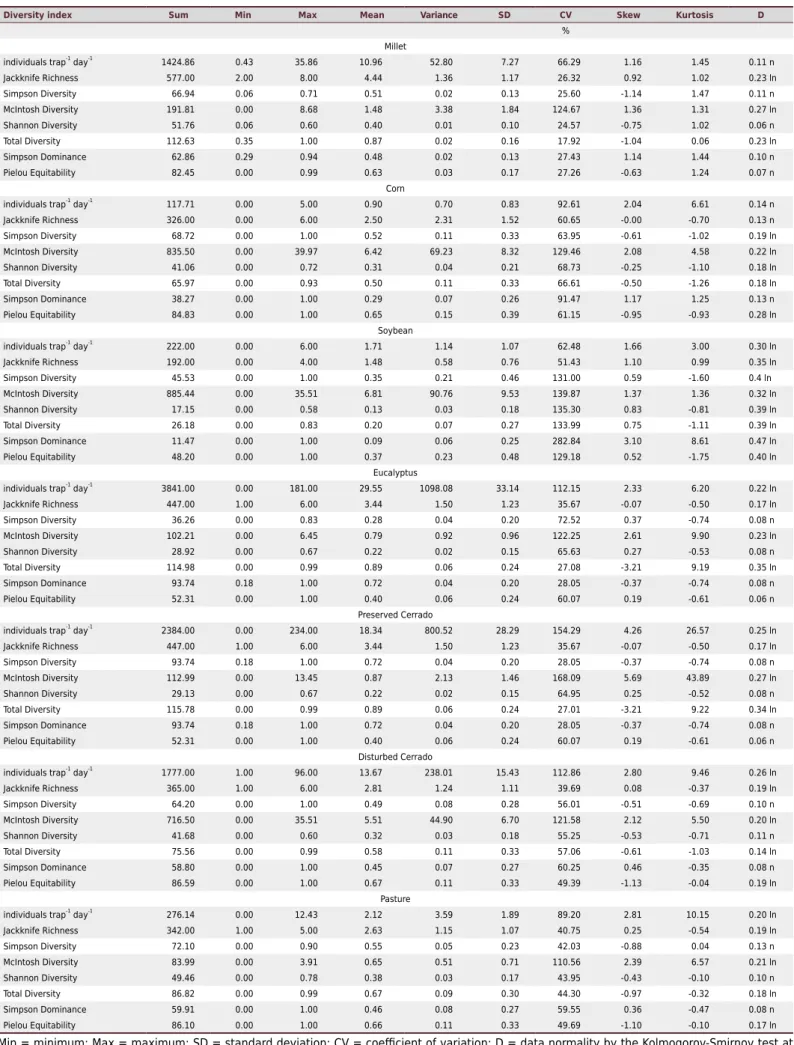
The main statistical parameters for biodiversity indices are described in table 4. In millet, according to the classification of Warrick and Nielsen (1980), the coefficient of variation (CV) values are considered medium, except for the indices individuals trap-1_day-1_{(CV = 66.29)}

and McIntosh diversity (CV = 124.67), which are considered high. For corn, all CV values are considered high (>60 %). In the soybean area, the CV values of the Simpson, McIntosh, Shannon diversity, total diversity, Simpson dominance, and Pielou equitability indices were above 100 %, which was also the case for the McIntosh index in all areas. High CV values are related to high standard deviations, explained by the aggregate behavior of the soil fauna and by intrinsic processes such as reproduction, feeding, migration, and dispersion of organisms. Thus, according to Warrick and Nielsen (1980), the CV values of soil properties can reach 1000 %.

Several authors report high CV values for soil variables. In a study on weed variability under different managements, Schaffrath et al. (2007) reported CV between 86.05 and 168.85 %. In an evaluation of the volumetric content of water in the soil, Siqueira et al. (2015a) reported a high CV range (97.60 - 106.8 %) for the different depths. However, Machado et al. (2006) attributed the high CV values to the sampling grid used.

There was variation regarding the minimum and maximum value of individuals in the areas. Only corn and soybean obtained a minimum value of zero in all indices. The highest mean was for individuals trap-1_day-1 _{in the eucalyptus area (29.55), followed by}

individuals trap-1_day-1_{in the preserved Cerrado (18.34); in both areas, the CV was greater}

than 100 %. According to Carvalho et al. (2002), skewness and kurtosis values between 0 and 3 indicate normal frequency. In this case, some indices presented no skewness and kurtosis values close to 0 and 3, indicating a lognormal distribution of these indices. For Isaaks and Srivastava (1989) and Cressie (1991), data normality is not a prerequisite for the use of geostatistics, whereas the stationarity of the semivariance is required.

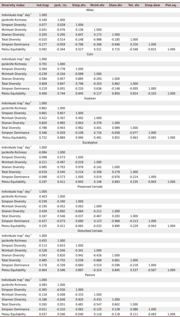
The linear correlation matrix showed negative values for some indices in all areas (Table 5). In millet, total diversity × individuals trap-1_day-1_{(r = -0.010) and Simpson}

diversity × Jackknife richness (r = -0.059) obtained very low and negative values, indicating an inverse association, that is, while an index grows other decreases. With the exception of preserved Cerrado, the correlation between Shannon index × Simpson diversity index for the other areas (millet r = 0647; corn r = 0.885, soybeans r = 0943; eucalyptus r = 0.976; disturbed Cerrado r = 0.942; pasture r = 0.920) remained high and positive, according to Santos classification (2007). The high correlation between Shannon diversity and Simpson diversity occurs because both indices take into account the total number of individuals within the sample, being these indices adequate to work with infinite communities, where it is only possible to determine diversity by sample means. The other correlations, with values between r = 0.1-0.5 or r = <0.1 are considered low.

(9)

Table 4. Statistical parameters for biodiversity indices in the studied areas

Diversity index Sum Min Max Mean Variance SD CV Skew Kurtosis D

%

Millet

individuals trap-1

day-1

1424.86 0.43 35.86 10.96 52.80 7.27 66.29 1.16 1.45 0.11 n

Jackknife Richness 577.00 2.00 8.00 4.44 1.36 1.17 26.32 0.92 1.02 0.23 ln

Simpson Diversity 66.94 0.06 0.71 0.51 0.02 0.13 25.60 -1.14 1.47 0.11 n

McIntosh Diversity 191.81 0.00 8.68 1.48 3.38 1.84 124.67 1.36 1.31 0.27 ln

Shannon Diversity 51.76 0.06 0.60 0.40 0.01 0.10 24.57 -0.75 1.02 0.06 n

Total Diversity 112.63 0.35 1.00 0.87 0.02 0.16 17.92 -1.04 0.06 0.23 ln

Simpson Dominance 62.86 0.29 0.94 0.48 0.02 0.13 27.43 1.14 1.44 0.10 n

Pielou Equitability 82.45 0.00 0.99 0.63 0.03 0.17 27.26 -0.63 1.24 0.07 n

Corn

individuals trap-1

day-1

117.71 0.00 5.00 0.90 0.70 0.83 92.61 2.04 6.61 0.14 n

Jackknife Richness 326.00 0.00 6.00 2.50 2.31 1.52 60.65 -0.00 -0.70 0.13 n

Simpson Diversity 68.72 0.00 1.00 0.52 0.11 0.33 63.95 -0.61 -1.02 0.19 ln

Shannon Diversity 41.06 0.00 0.72 0.31 0.04 0.21 68.73 -0.25 -1.10 0.18 ln

Total Diversity 65.97 0.00 0.93 0.50 0.11 0.33 66.61 -0.50 -1.26 0.18 ln

Simpson Dominance 38.27 0.00 1.00 0.29 0.07 0.26 91.47 1.17 1.25 0.13 n

Pielou Equitability 84.83 0.00 1.00 0.65 0.15 0.39 61.15 -0.95 -0.93 0.28 ln

Soybean

individuals trap-1 day-1 222.00 0.00 6.00 1.71 1.14 1.07 62.48 1.66 3.00 0.30 ln

Jackknife Richness 192.00 0.00 4.00 1.48 0.58 0.76 51.43 1.10 0.99 0.35 ln

Simpson Diversity 45.53 0.00 1.00 0.35 0.21 0.46 131.00 0.59 -1.60 0.4 ln

Shannon Diversity 17.15 0.00 0.58 0.13 0.03 0.18 135.30 0.83 -0.81 0.39 ln

Total Diversity 26.18 0.00 0.83 0.20 0.07 0.27 133.99 0.75 -1.11 0.39 ln

Simpson Dominance 11.47 0.00 1.00 0.09 0.06 0.25 282.84 3.10 8.61 0.47 ln

Pielou Equitability 48.20 0.00 1.00 0.37 0.23 0.48 129.18 0.52 -1.75 0.40 ln

Eucalyptus

individuals trap-1

day-1

3841.00 0.00 181.00 29.55 1098.08 33.14 112.15 2.33 6.20 0.22 ln

Jackknife Richness 447.00 1.00 6.00 3.44 1.50 1.23 35.67 -0.07 -0.50 0.17 ln

Simpson Diversity 36.26 0.00 0.83 0.28 0.04 0.20 72.52 0.37 -0.74 0.08 n

Shannon Diversity 28.92 0.00 0.67 0.22 0.02 0.15 65.63 0.27 -0.53 0.08 n

Simpson Dominance 93.74 0.18 1.00 0.72 0.04 0.20 28.05 -0.37 -0.74 0.08 n

Pielou Equitability 52.31 0.00 1.00 0.40 0.06 0.24 60.07 0.19 -0.61 0.06 n

Preserved Cerrado individuals trap-1

day-1

2384.00 0.00 234.00 18.34 800.52 28.29 154.29 4.26 26.57 0.25 ln

Jackknife Richness 447.00 1.00 6.00 3.44 1.50 1.23 35.67 -0.07 -0.50 0.17 ln

Simpson Diversity 93.74 0.18 1.00 0.72 0.04 0.20 28.05 -0.37 -0.74 0.08 n

Shannon Diversity 29.13 0.00 0.67 0.22 0.02 0.15 64.95 0.25 -0.52 0.08 n

Simpson Dominance 93.74 0.18 1.00 0.72 0.04 0.20 28.05 -0.37 -0.74 0.08 n

Pielou Equitability 52.31 0.00 1.00 0.40 0.06 0.24 60.07 0.19 -0.61 0.06 n

Disturbed Cerrado

individuals trap-1

day-1

1777.00 1.00 96.00 13.67 238.01 15.43 112.86 2.80 9.46 0.26 ln

Jackknife Richness 365.00 1.00 6.00 2.81 1.24 1.11 39.69 0.08 -0.37 0.19 ln

Simpson Diversity 64.20 0.00 1.00 0.49 0.08 0.28 56.01 -0.51 -0.69 0.10 n

Shannon Diversity 41.68 0.00 0.60 0.32 0.03 0.18 55.25 -0.53 -0.71 0.11 n

Simpson Dominance 58.80 0.00 1.00 0.45 0.07 0.27 60.25 0.46 -0.35 0.08 n

Pasture

individuals trap-1

day-1

276.14 0.00 12.43 2.12 3.59 1.89 89.20 2.81 10.15 0.20 ln

Jackknife Richness 342.00 1.00 5.00 2.63 1.15 1.07 40.75 0.25 -0.54 0.19 ln

Simpson Diversity 72.10 0.00 0.90 0.55 0.05 0.23 42.03 -0.88 0.04 0.13 n

Shannon Diversity 49.46 0.00 0.78 0.38 0.03 0.17 43.95 -0.43 -0.10 0.10 n

Simpson Dominance 59.91 0.00 1.00 0.46 0.08 0.27 59.55 0.36 -0.47 0.08 n

Min = minimum; Max = maximum; SD = standard deviation; CV = coefficient of variation; D = data normality by the Kolmogorov-Smirnov test at

(10)

Table 5. Linear correlation matrix for the biodiversity indexes in the studied areas

Diversity index Ind.trap Jack. ric. Simp.div. McInt.div Shan.div Tot. div Simp.dom Piel.eq.

Millet Individuals trap-1 day-1 1.000

Jackknife Richness 0.160 1.000

Simpson Diversity 0.077 0.028 1.000

McIntosh Diversity 0.041 -0.476 0.136 1.000

Shanon Diversity 0.205 0.295 0.647 0.173 1.000

Total Diversity -0.010 0.514 -0.148 -0.988 -0.185 1.000

Simpson Dominance -0.177 -0.059 -0.706 -0.306 -0.946 0.316 1.000

Pielou Equitability 0.092 -0.344 0.527 0.521 0.715 -0.548 -0.815 1.000

Corn Individuals trap-1

day-1

1.000

McIntosh Diversity -0.239 -0.244 -0.099 1.000

Shanon Diversity 0.584 0.957 0.885 -0.293 1.000

Total Diversity 0.609 0.847 0.796 -0.353 0.862 1.000

Simpson Dominance 0.219 0.001 -0.220 0.636 -0.148 -0.005 1.000

Pielou Equitability 0.400 0.744 0.945 -0.117 0.850 0.814 -0.103 1.000

Soybean Individuals trap-1

day-1

1.000

McIntosh Diversity 0.422 0.307 0.492 1.000

Shanon Diversity 0.820 0.965 0.943 0.379 1.000

Total Diversity 0.788 0.943 0.962 0.401 0.989 1.000

Simpson Dominance 0.346 -0.029 -0.108 0.716 -0.058 -0.077 1.000

Pielou Equitability 0.722 0.869 0.990 0.491 0.952 0.963 -0.065 1.000

Eucalyptus Individuals trap-1

day-1

1.000

Jackknife Richness -0.084 1.000

McIntosh Diversity 0.211 -0.497 -0.019 1.000

Total Diversity -0.019 0.545 0.214 -0.358 0.279 1.000

Simpson Dominance -0.098 -0.573 -1.000 0.019 -0.976 -0.214 1.000

Pielou Equitability 0.197 0.411 0.943 0.146 0.893 0.235 -0.943 1.000

Preserved Cerrado Individuals trap-1

day-1

1.000

Simpson Diversity -0.239 -0.340 1.000

McIntosh Diversity -0.195 -0.452 0.063 1.000

Shanon Diversity 0.439 0.692 -0.664 -0.212 1.000

Total Diversity 0.167 0.546 -0.037 -0.467 0.283 1.000

Simpson Dominance -0.427 -0.573 0.690 0.123 -0.968 -0.213 1.000

Pielou Equitability 0.335 0.411 -0.665 -0.033 0.890 0.229 -0.943 1.000

Disturbed Cerrado Individuals trap-1 day-1 1.000

Simpson Diversity -0.113 0.653 1.000

McIntosh Diversity -0.328 -0.506 -0.341 1.000

Total Diversity 0.485 0.755 0.558 -0.668 0.661 1.000

Simpson Dominance 0.278 -0.339 -0.660 0.510 -0.596 -0.218 1.000

Pielou Equitability -0.064 0.546 0.897 -0.314 0.845 0.537 -0.507 1.000

Pasture Individuals trap-1

day-1

1.000

Simpson Diversity -0.365 -0.030 1.000

McIntosh Diversity -0.116 0.008 -0.333 1.000

Shannon Diversity -0.186 -0.048 0.920 -0.433 1.000

Total Diversity 0.265 0.051 0.481 -0.547 0.602 1.000

Simpson Dominance -0.011 -0.310 0.062 -0.120 0.128 0.086 1.000

Pielou Equitability 0.037 0.546 -0.040 0.116 -0.118 -0.111 -0.493 1.000

Ind.trap: Individuals trap-1 day-1

(11)

McIntosh, Shannon diversity, Simpson dominance, and Pielou equitability in the corn area; Simpson, McIntosh diversity, total diversity in soybean area; Simpson, McIntosh, Shannon diversity, total diversity, Simpson dominance, and Pielou equitability in the eucalyptus area; individuals trap-1_day-1_{, jackknife richness, Simpson diversity, McIntosh diversity, total diversity,}

and Pielou equitability in the preserved Cerrado area; Simpson diversity, Shannon diversity, Simpson dominance, and Pielou equitability in the disturbed Cerrado; individuals trap-1_day-1_,

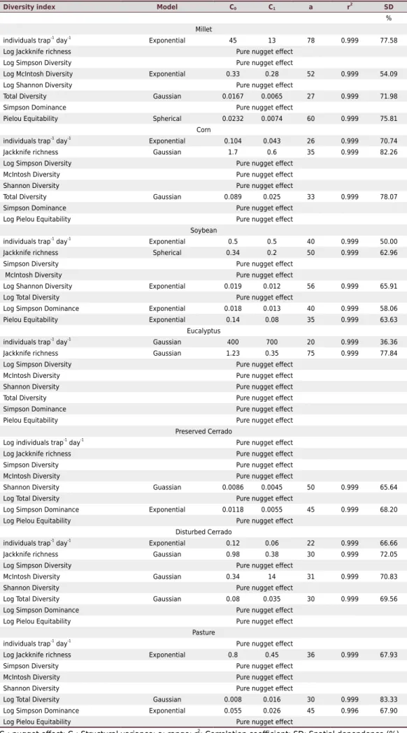
Simpson, McIntosh, Shannon index, and Pielou equitability in the pasture area. Siqueira et al. (2016) evaluating the variability of weeds in a no-tillage system obtained a pure nugget effect for the Shannon diversity index, the same occurred in the present study for millet, corn, eucalyptus, disturbed Cerrado, and pasture areas. The pure nugget effect indicates that 3 m spacing was not sufficient to detect spatial variability (Vieira, 2000).

The other indices with spatial variability were fitted to a geostatistical model, Gaussian, spherical or exponential. For the millet only the Pielou equitability was adjusted to the spherical model, individuals trap-1_day-1

and McIntosh diversity were fitted to the exponential model and total diversity to the Gaussian model (Table 6). Gholami et al. (2016) studying the spatial variability of the soil macrofauna associated to abiotic factors in a riparian forest in south-western Iran, it adjusted the exponential model to the index of uniformity, richness and diversity, and the spherical model to soil macrofauna abundance. Several authors describe that the spherical model is the one that best fits the soil and plants data (Cambardella et al., 1994; Vieira, 2000; Siqueira et al., 2008; Siqueira et al., 2009; Chiba et al., 2010; Silva et al., 2014; Siqueira et al., 2015b).

According to the classification of Cambardella et al. (1994), the spatial dependence degree for the individuals trap-1_day-1_{index and Pielou equitability in the millet area is high (above 75 %).}

For soybean and preserved Cerrado area, the spatial dependence remained the median (25 to 75 %). The highest value of nugget effect (C0) was for individuals trap

-1_day-1_{in eucalyptus}

(C0 = 400), and the lowest value was for total diversity (C0 = 0.008) in the pasture, which

indicates good representativeness of the semivariogram fitting parameter. According to Carvalho et al. (2001), high values of nugget effect indicate discontinuity between the samples. The range of values (a) ranged from 20 m individuals trap-1_day-1_{in eucalyptus to 78 m}

individuals trap-1_day-1_{in millet. The determination of the range values is needed to know}

to what point the samples are correlated with each other and the maximum spatial dependence distance between the samples (Vieira, 2000). For Carvalho et al. (2003), based on the range of spatial dependence, future samplings can be delineated, provided the same conditions are repeated. In a study on the spatial variability of the diversity indices of soil macrofauna, Gholami et al. (2016) found range values varying from 952 m for diversity to 2,967 m for the uniformity index.

Soil arthropods play a relevant role with regard to the ecosystem quality. However, their abundance and richness may be affected by land use and soil management (Lima et al., 2010), and by physical and chemical properties (Majer et al., 2007; Rousseau et al., 2014; Bedano et al., 2016). According to Birkhofer et al. (2010), the biotic relations also contribute to the formation of spatial patterns. In this sense, the presence of cover crops favors species of the soil epigeal fauna that are specialized and sensitive to abiotic alterations, e.g., Acari, Araneae, Diplura, Formicidae, and Poduromorpha. This occurs due to food offer, microclimate, and natural shelter (Batista et al., 2014; Gholami et al., 2014; Franco et al., 2016).

Soil use and management are directly related to spatial patterns of soil fauna (Ettema and Wardle, 2002; Bardgett and van der Putten, 2014). Therefore, it is possible to describe the greatest differences in the spatial distribution of soil macrofauna, mainly in preserved and disturbed Cerrado because the soil fauna is sensitive to minimal alterations caused by inappropriate soil use and management.

(12)

Table 6. Semivariogram fitting parameters for biodiversity indices in the studied areas

Diversity index Model C0 C1 a r

2

SD

% Millet

individuals trap-1

day-1

Exponential 45 13 78 0.999 77.58

Log Jackknife richness Pure nugget effect

Log Simpson Diversity Pure nugget effect

Log McIntosh Diversity Exponential 0.33 0.28 52 0.999 54.09

Log Shannon Diversity Pure nugget effect

Total Diversity Gaussian 0.0167 0.0065 27 0.999 71.98

Simpson Dominance Pure nugget effect

Pielou Equitability Spherical 0.0232 0.0074 60 0.999 75.81

Corn individuals trap-1

day-1

Exponential 0.104 0.043 26 0.999 70.74

Jackknife richness Gaussian 1.7 0.6 35 0.999 82.26

McIntosh Diversity Pure nugget effect

Shannon Diversity Pure nugget effect

Total Diversity Gaussian 0.089 0.025 33 0.999 78.07

Log Pielou Equitability Pure nugget effect

Soybean individuals trap-1

day-1

Exponential 0.5 0.5 40 0.999 50.00

Jackknife richness Spherical 0.34 0.2 50 0.999 62.96

Simpson Diversity Pure nugget effect

Log Shannon Diversity Exponential 0.019 0.012 56 0.999 65.91

Log Total Diversity Pure nugget effect

Log Simpson Dominance Exponential 0.018 0.013 40 0.999 58.06

Pielou Equitability Exponential 0.14 0.08 35 0.999 63.63

Eucalyptus individuals trap-1

day-1

Gaussian 400 700 20 0.999 36.36

Total Diversity Pure nugget effect

Pielou Equitability Pure nugget effect

Preserved Cerrado Log individuals trap-1

day-1 Pure nugget effect

Log Jackknife richness Pure nugget effect

Shannon Diversity Guassian 0.0086 0.0045 50 0.999 65.64

Log Total Diversity Pure nugget effect

Disturbed Cerrado

individuals trap-1 day-1 Exponential 0.12 0.06 22 0.999 66.66

McIntosh Diversity Gaussian 0.34 14 31 0.999 70.83

Log Total Diversity Gaussian 0.08 0.035 30 0.999 69.56

Log Simpson Dominance Pure nugget effect

Pasture

individuals trap-1 day-1 Pure nugget effect

Log Jackknife richness Exponential 0.8 0.45 36 0.999 67.93

Log Total Diversity Gaussian 0.008 0.016 30 0.999 83.33

C0: nugget effect; C1: Structural variance; a: range; r

(13)

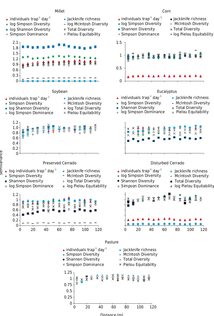
Figure 2. Scaled semivariograms for biodiversity indices in the studied areas.

Semivarianc

e

Millet Corn

Soybean Eucalyptus

Preserved Cerrado Disturbed Cerrado

0 0.3 0.6 0.9 1.2 1.5 1.8 2.1

individuals trap-1_day-1 _{Jackknife richness}

log Simpson Diversity log McIntosh Diversity

log Shannon Diversity Total Diversity

Simpson Dominance Pielou Equitability

0 0.5 1 1.5

individuals trap-1 day-1 Jackknife richness

log Simpson Diversity McIntosh Diversity

Shannon Diversity Total Diversity

Simpson Dominance log Pielou Equitability

Simpson Diversity McIntosh Diversity

log Shannon Diversity log Total Diversity

log Simpson Dominance Pielou Equitability

individuals trap-1 day-1 Jackknife richness

log Simpson Dominance Pielou Equitability

0 0.2 0.4 0.6 0.8 1 1.2 0 0.2 0.4 0.6 0.8 1.0 1.2

0 20 40 60 80 100 120

log individuals trap-1_day-1 _{Jackknife richness}

Shannon Diversity log Total Diversity

log Simpson Dominance log Pielou Equitability

0 20 40 60 80 100 120

individuals trap-1_day-1

Jackknife richness

Simpson Dominance log Pielou Equitability

Pasture

Distance (m) 0

0.25 0.5 0.75 1 1.25

0 20 40 60 80 100 120

(14)

it favors the comparison and comprehension of the spatial variability of the studied diversity indices.

For the areas of soybean and pasture, biodiversity indices suggested similarity of spatial variability. However, the Shannon diversity, Simpson diversity, McIntosh diversity, and jackknife richness indices in millet were more dispersed than the other indices of this crop area. The same was observed for individuals trap-1_day-1_{in the corn area; Shannon diversity}

in eucalyptus; McIntosh diversity in the preserved Cerrado; and individuals trap-1_day-1

and Jackknife richness in the disturbed Cerrado. The greatest differences described for soil macrofauna diversity indices by the scaled semivariogram are a result of the soil management, disturbance degree, and sensitivity of macrofauna groups to food availability.

Therefore, the semivariance of the Shannon index was higher for millet than the other semivariance values of the other indices for the area, separating this index from the others. In the other cases, the semivariance was close to zero, and lower than the indices with similar variability.

This dispersion may be explained by the parameters used to determine the indices. The individuals trap-1_day-1_{indices take the number of individuals collected in a sample of seven}

days into consideration, so this value always tends to be higher or equal to the others. With regard to the Shannon, Simpson, and McIntosh indices, the total number of species in a given sample is considered, and, specifically in the case of McIntosh diversity, the square root of the sum of the number of individuals, which explains the high values of semivariance in the Shannon and Simpson indices and the low semivariance of McIntosh’s index in millet.

Another explanation for the variation in semivariance values may be related to the number of individuals collected in each area and their distribution among the samples. In an evaluation of the Shannon and Simpson diversity indices in weeds, Siqueira et al. (2016) observed similar spatial variability of these indices.

CONCLUSIONS

Soil management and land use affected the patterns of soil fauna abundance, richness and diversity. The presence of groups such as Araneae, Diplura, and Poduromorpha indicated the ecological equilibrium, quality and sustainability of the agricultural systems studied. Geostatistical techniques satisfactorily analyzed the spatial dynamics of soil fauna in the seven studied areas. The spatial variability of all indices in the soybean and pasture area is similar, with close semivariance values.

ACKNOWLEDGMENTS

The authors are indebted to the Fapema (Foundation for Research and Scientific and Technological Development of Maranhão, Brazil) for the financial support of the project (Apcinter-02587/14, BATI-02985/14, Universal-00735/15, BEPP-01301/15, APEC 01697/15, BM-01267/15, Fapema/05232/15 and BD-01343/15). Authors would like to thank CNPq (Conselho Nacional de Desenvolvimento Científico e Tecnológico) for the grant awarded to the second and fifth author.

REFERENCES

Aquino AM. Manual para macrofauna do solo. Seropédica: Embrapa Agrobiologia; 2001. (Documentos 130).

(15)

Bardgett RD, van der Putten WH. Belowground biodiversity and ecosystem functioning. Nature. 2014;515:505-11. https://doi.org/10.1038/nature13855

Baretta D, Santos JCP, Mafra AL, Wildner LP, Miquelluti DJ. Fauna edáfica avaliada por

armadilhas e catação manual afetada pelo manejo do solo na região oeste catarinense. Rev Cienc Agroveterinarias. 2003;2:97-106.

Basso FC, Andreotti M, Carvalho MP, Lodo BN. Relações entre produtividade de sorgo forrageiro e atributos físicos e teor de matéria orgânica de um Latossolo do Cerrado. Pesq Agropec Trop. 2011;41:135-44. https://doi.org/10.5216/pat.v41i1.7099

Batista I, Correia MEF, Pereira MG, Bieluczyk W, Schiavo JA, Rouws JRC. Frações oxidáveis do

carbono orgânico total e macrofauna edáfica em sistema de integração lavoura-pecuária. Rev

Bras Cienc Solo. 2014;38:797-809. https://doi.org/10.1590/S0100-06832014000300011

Bedano JC, Domínguez A, Arolfo R, Wall LG. Effect of good agricultural practices under no-till on litter and soil invertebrates in areas with different soil types. Soil Till Res. 2016;158:100-9.

https://doi.org/10.1016/j.still.2015.12.005

Birkhofer K, Scheu S, Wiegand D. Assessing spatiotemporal predator-prey patterns in heterogeneous habitats. Basic Appl Ecol. 2010;11:486-94. https://doi.org/10.1016/j.baae.2010.06.010

Blanchart E, Villenave C, Viallatoux A, Barthès B, Girardin C, Azontonde A, Feller C. Long-term

effect of a legume cover crop (Mucuna pruriens var. utilis) on the communities of soil macrofauna and nematofauna, under maize cultivation, in southern Benin. Eur J Soil Biol. 2006;42:S136-44. https://doi.org/10.1016/j.ejsobi.2006.07.018

Bonnin JJ, Mirás-Avalos JM, Lanças KP, González AP, Vieira SR. Spatial variability of soil

penetration resistance influenced by season of sampling. Bragantia. 2010;69:163-73.

https://doi.org/10.1590/S0006-87052010000500017

Bottega EL, Queiroz DM, Pinto FAC, Souza CMA. Variabilidade espacial de atributos do solo em sistema de semeadura direta com rotação de culturas no cerrado brasileiro. Rev Cienc Agron. 2013;44:1-9. https://doi.org/10.1590/S1806-66902013000100001

Bottinelli N, Jouquet P, Capowiez Y, Podwojewski P, Grimaldi M, Peng X. Why is the influence

of soil macrofauna on soil structure only considered by soil ecologists? Soil Till Res. 2015;146:118-24. https://doi.org/10.1016/j.still.2014.01.007

Camargo OA, Moniz AC, Jorge JA, Valadares JMAS. Métodos de análise química, mineralógica e física de solos do Instituto Agronômico de Campinas. Campinas: Instituto Agronômico; 2009. (Boletim técnico, 106).

Cambardella CA, Moorman TB, Parkin TB, Karlem DL, Novak JM, Turco RF, Konopka AE. Field-scale variability of soil properties in central Iowa soils. Soil Sci Soc Am J. 1994;58:1501-11. https://doi.org/10.2136/sssaj1994.03615995005800050033x

Carvalho JR, Vieira SR, Marinho PR, Dechen SCF, Maria IC, Pott CA, Dufranc G. Avaliação da variabilidade espacial de parâmetros físicos do solo sob semeadura direta em São Paulo, Brasil. Campinas: Embrapa; 2001. p. 1-4. (Comunicado Técnico).

Carvalho JRP, Silveira PM, Vieira SR. Geoestatística na determinação da variabilidade espacial de características químicas do solo sob diferentes preparos. Pesq Agropec Bras. 2002;37:1151-9. https://doi.org/10.1590/S0100-204X2002000800013

Carvalho LA, Meurer I, Silva Junior CA, Santos CFB, Libardi PL. Spatial variability of soil potassium in sugarcane areas subjected to the application of vinasse. An Acad Bras Cienc. 2014;86:1999-2011. https://doi.org/10.1590/0001-3765201420130319

Carvalho MP, Takeda EY, Freddi OS. Variabilidade espacial de atributos de um solo sob videira em Vitória Brasil (SP). Rev Bras Cienc Solo. 2003;27:695-703. https://doi.org/10.1590/S0100-06832003000400014

(16)

Correia MEF. Potencial de utilização dos atributos das comunidades de fauna do solo e de grupos chave de invertebrados como bioindicadores de manejo de ecossistemas. Seropédica: Embrapa Agrobiologia; 2002. (Documentos, 157).

Cressie NAC. Statistics for spatial data. New York: John Wiley & Sons, Inc.; 1991.

Crusciol CAC, Soratto RP, Borghi E, Matheus GP. Benefits of integrating crops and tropical

pastures as systems of production. Better Crops With Plant Food. 2010;94:14-6.

Cunha EQ, Stone LF, Didonet AD, Ferreira EPB, Moreira JAA, Leandro WM. Atributos químicos de

solo sob produção orgânica influenciados pelo prepare e por plantas de cobertura. Rev Bras Eng

Agric Ambient. 2011;15:1021-9. https://doi.org/10.1590/S1415-43662011001000005 Domínguez A, Bedano JC, Becker AR, Arolfo RV. Organic farming fosters agroecosystem functioning in Argentinian temperate soils: evidence from litter decomposition and soil fauna. Appl Soil Ecol. 2014;83:170-6. https://doi.org/10.1016/j.apsoil.2013.11.008

Ettema CH, Wardle DA. Spatial soil ecology. Trends Ecol Evol. 2002;17:177-83. https://doi.org/10.1016/S0169-5347(02)02496-5

Franco ALC, Bartz MLC, Cherubin MR, Baretta D, Cerri CEP, Feigl BJ, Wall DH, Davies CA, Cerri CC. Loss of soil (macro)fauna due to the expansion of Brazilian sugarcane acreage. Sci Total Environ. 2016;563-564:160-8. https://doi.org/10.1016/j.scitotenv.2016.04.116

Gholami SH, Mahini AS, Hosseini SM, Mohammadi J, Sayad E. Assessment of vegetation density and soil macrofauna relationship in riparian forest of Karkhe River for determination of rivers

buffer zone. Iranian J Appl Ecol. 2014;7:13-26.

Gholami S, Sayad E, Gebbers R, Schirrmann M, Joschko M, Timmer J. Spatial analysis of riparian forest soil macrofauna and its relation to abiotic soil properties. Pedobiologia. 2016;59:27-36. https://doi.org/10.1016/j.pedobi.2015.12.003

Isaaks EH, Srivastava RM. An introduction to applied geostatistics. New York: Oxford University Press; 1989.

Jeffers JNR. An introduction to system analysis: with ecological applications. London: University

Park Press; 1978.

Journel AG, Huijbregts CJ. Mining geostatistics. London: Academic Press; 1978.

Lawrence JF. Key to hexapod orders and some other arthropod groups. In: Naumann ID, editor. Systematic and applied entomology: an introduction. Carlton: Melbourne University Press; 1994. p. 223-31.

Lima SS, Aquino AM, Leite LFC, Velásquez E, Lavelle P. Relação entre macrofauna edáfica e

atributos químicos do solo em diferentes agroecossistemas. Pesq Agropec Bras. 2010;45:322-31. https://doi.org/10.1590/S0100-204X2010000300013

Machado PLOA, Bernadi ACC, Valencia LIO, Molin JP, Gimenez LM, Silva CA, Andrade AG, Madari BE, Meirelles MSP. Mapeamento da condutividade elétrica e relação com a argila de Latossolo sob plantio direto. Pesq Agropec Bras. 2006;41:1023-31. https://doi.org/10.1590/S0100-204X2006000600019

Magurran AE. Ecological diversity and its measurement. New Jersey: Princeton University Press; 1988. Majer JD, Brennan KEC, Moir ML. Invertebrates and the restoration of a forest ecosystem: 30 years of research following bauxite mining in Western Australia. Restor Ecol. 2007;15:S104-15. https://doi.org/10.1111/j.1526-100X.2007.00298.x

Montanari R, Carvalhos MP, Andreotti M, Dalchiavon FC, Lovera LH, Honorato MAO. Aspectos da produtividade do feijão correlacionados com atributos físicos do solo sob elevado nível tecnológico de manejo. Rev Bras Cienc Solo. 2010;34:1811-22. https://doi.org/10.1590/S0100-06832010000600005

(17)

Moura EG, Aguiar ACF, Piedade AR, Rousseau GX. Contribution of legume tree residues and macrofauna to the improvement of abiotic soil properties in the eastern Amazon. Appl Soil Ecol. 2015;86:91-9. https://doi.org/10.1016/j.apsoil.2014.10.008

Paul BK, Vanlauwe B, Ayuke F, Gassner A, Hoogmoed M, Hurisso TT, Koala S, Lelei D,

Ndabamenye T, Six J, Pulleman MM. Medium-term impact of tillage and residue management on soil aggregate stability, soil carbon and crop productivity. Agr Ecosyst Environ. 2013;164:14-22. https://doi.org/10.1016/j.agee.2012.10.003

Pedroso AJS, Ruivo MLP, Piccinin JL, Okumura RS, Birani SM, Silva Junior ML, Melo VS, Costa AR,

Albuquerque MPF. Chemical attributes of Oxisol under different tillage systems in Northeast of

Pará. Afr J Agr Res. 2016;11:4947-52. https://doi.org/10.5897/AJAR2016.11688

R Development Core Team. R: A language and environment for statistical computing. R Foundation for Statistical Computing, Vienna, Austria; 2009. Available at: http://www.R-project.org/.

Rafael JA, Melo GAR, Carvalho CJB, Casari SA, Constantino R, editores. Insetos do Brasil: diversidade e taxonomia. Ribeirão Preto: Holos Editora; 2012.

Ribeiro LS, Oliveira IR, Dantas JS, Silva CV, Silva GB, Azevedo JR. Variabilidade espacial de atributos físicos de solo coeso sob sistemas de manejo convencional e plantio direto. Pesq Agropec Bras. 2016;51:1699-702. https://doi.org/10.1590/S0100-204X2016000900071

Rodrigues WC. DivEs - Diversidade de espécies v3.0: guia do usuário. Entomologistas do Brasil; 2015. Disponível em: http://dives.ebras.bio.br.

Rousseau GX, Silva PRS, Celentano D, Carvalho CJR. Macrofauna do solo em uma

cronosequência de capoeiras, florestas e pastos no Centro de Endemismo Belém, Amazônia

Oriental. Acta Amaz. 2014;44:499-512. https://doi.org/10.1590/1809-4392201303245 Santos C. Estatística descritiva: manual de auto-aprendizagem. Lisboa: Edições Sílabo; 2007.

Schaffrath VR, Tormena CA, Gonçalves ACA, Oliveira Junior RS. Variabilidade espacial de plantas

daninhas em dois sistemas de manejo de solo. Rev Bras Eng Agric Ambient. 2007;11:53-60. https://doi.org/10.1590/S1415-43662007000100007

Silva J, Assis Junior RN, Matias SSR, Tavares RC, Andrade FR, Camacho-Tamayo JH. Using geostatistics to evaluate the physical attributes of a soil cultivated with sugarcane. Rev Cienc Agrar. 2014;57:186-93. https://doi.org/10.4322/rca.2014.013

Siqueira GM, Dafonte JD, Valcárcel AM. Correlación espacial entre malas hierbas en una pradera y su relación con la conductividad eléctrica aparente del suelo (CEA). Planta Daninha.

2015a;33:631-41. https://doi.org/10.1590/S0100-83582015000400002

Siqueira GM, Silva EFF, Paz-Ferreiro J. Land use intensification effects in soil arthropod community of an Entisol in Pernambuco state, Brazil. The Scientific World Journal.

2014;2014:1-7. https://doi.org/10.1155/2014/625856

Siqueira GM, Silva EFF, Vidal-Válquez E, Paz-González A. Multifractal and joint multifractal analysis of general soil properties and altitude along a transect. Biosyst Eng. 2017. In press. https://doi.org/10.1016/j.biosystemseng.2017.08.024

Siqueira GM, Silva JS, Bezerra JM, Silva EFF, Dafonte JD, Melo RF. Estacionariedade do conteúdo de água de um Espodossolo Humilúvico. R Bras Eng Agric Ambient. 2015b;19:439-48.

https://doi.org/10.1590/1807-1929/agriambi.v19n5p439-448

Siqueira GM, Silva RA, Aguiar ACF, Costa MKL, Silva EFF. Spatial variability of weeds in an Oxisol under no-tillage system. Afr J Agric Res. 2016;11:2569-76. https://doi.org/10.5897/AJAR2016.11120

Siqueira GM, Vieira SR, Ceddia MB. Variabilidade de atributos físicos do solo determinados por métodos diversos. Bragantia. 2008;67:203-11. https://doi.org/10.1590/S0006-87052008000100025

(18)

Soil Survey Staff. Soil taxonomy: a basic system of soil classification for making and interpreting

soil surveys. 2nd ed. Washington, DC: United States Department of Agriculture, Natural Resources Conservation Service; 1999. (Agricultural Handbook, 436).

Vasconcellos RLF, Segat JC, Bonfim JA, Baretta D, Cardoso EJBN. Soil macrofauna as an indicator of soil quality in an undisturbed riparian forest and recovering sites of different ages. Eur J Soil

Biol. 2013;58:105-12. https://doi.org/10.1016/j.ejsobi.2013.07.001

Vieira SR. Geoestatística em estudos de variabilidade espacial do solo. In: Novais RF, Alvarez V VH, Schaefer CEGR. Tópicos em Ciência do Solo. Viçosa, MG: Sociedade Brasileira de Ciência do Solo; 2000. v.1. p. 1-54.

Vieira SR, Tillotson PM, Biggar JW, Nielsen DR. Scaling of semivariograms and the

kriging estimation of field-measured properties. Rev Bras Cienc Solo. 1997;21:525-33.

https://doi.org/10.1590/S0100-06831997000400001

Vries FT, Thébault E, Liiri M, Birkhofer K, Tsiafouli MA, Bjørnlund L, Jørgensen HB, Brady MV, Christensen S, Ruiter PC, d’Hertefeldt T, Frouz J, Hedlund K, Hemerik L, Holk WHG, Hotes S, Mortimer SN, Setälä H, Sgardelis SP, Uteseny K, van der Putten WH, Wolters V, Bardgett RD. Soil food web properties explain ecosystem services across European land use systems. P Natl A Sci USA. 2013;110:14296-301. https://doi.org/10.1073/pnas.1305198110

Wagg C, Bender SF, Widmer F, van der Heijden MGA. Soil biodiversity and soil community composition determine ecosystem multifunctionality. P Natl A Sci USA. 2014;111:5266-70. https://doi.org/10.1073/pnas.1320054111

Warrick AW, Nielsen DR. Spatial variability of soil physical properties in the field. In: Hillel D,

editor. Applications of soil physics. New York: Academic Press; 1980. p. 319-44.

Zonta JH, Brandão ZN, Medeiros JC, Sana RS, Sofiatti V. Variabilidade espacial da fertilidade