A DECENTRALIZED APPROACH TO GENERAL
EQUILIBRIUM ANALYSIS
Emanuel R. Leão
Julho 2008
WP nº 2008/66
DOCUMENTO DE TRABALHO WORKING PAPERD I N Â M I A C E N T R O D E E S T U D O S S O B R E A M U D A N Ç A S O C I O E C O N Ó M I C A
Emanuel R. Leão
1W
W
P
P
n
n
º
º
2
2
0
0
0
0
8
8
/
/
6
6
6
6
J
J
u
u
l
l
h
h
o
o
d
d
e
e
2
2
0
0
0
0
8
8
1 Departament of Economics, Instituto Superior de Ciências do Trabalho e da Empresa and Dinâmia – Centro de Estudos sobre a Mudança Socioeconómica, Avenida das Forças Armadas, 1649-026 Lisboa, Portugal, Phone: 00351217903236, Fax: 00351217903933 - E-mail: [email protected]
A Abbssttrraacctt 1 1.. IINNTTRROODDUUCCTTIIOONN 3 3 2 2.. TTHHEE MMOODDEELL 3 3 3 3.. TTHHEE TTYYPPIICCAALL FFIIRMRM’’SS BBEEHHAAVVIIOOUURR 6 6 4 4.. TTHHEE TTYYPPIICCAALL HHOOUUSSEEHHOOLLDD’’S S BBEEHHAAVVIIOOUURR 9 9 5 5.. TTHHEE MMAARRKKEETT CCLLEEAARRIINNGG CCOONNDDIITTIIOONNSS 1515 6 6..TTHHEE CCOOMMPPEETTIITTIIVVEE EEQQUUIILLIIBBRRIIUUMM 1616 7 7.. TTHHEE CCOOMMPPEETTIITTIIVVEE EEQQUUIILILIBBRRIIUMUM AASSSSUUMMIINNGG RRAATTIIONONAALL EEXXPPEECCTTAATTIIOONNSS 1818 8 8.. WWAALLRRAASS’’ LLAAWW 2222 9 9.. TTHHEE SSEECCOONNDD WWEELLFFAARREE TTHHEEOORREEMM 2323 1 100.. NNEEAARR SSTTEEAADDYY--SSTTAATTEE DDYYNNAAMMIICCSS 2626 1 111.. CCAALLIIBBRRAATTIIOONN 2828 1 122.. RREESSPPOONNSSEE OOFF TTHHEE MMOODDEELL TTOO EEXOXOGGEENNOOUUSS SSHHOOCCKKSS 3030 1 133.. CCOONNCCLLUUSSIIOONN 3434 R REEFFEERREENNCCEESS 4141 A ANNNNEEXXEESS
1
Introduction
In this paper we develop a decentralized zero growth version of the model in King, Plosser and Rebelo (1988). By zero growth model we mean a model where physical output is constant in the steady-state. Note that, for the purposes of simulation, King, Plosser and Rebelo also transform their exogenous growth model into a model which is essentially a zero growth model.
Our use of a decentralized version can also be explained. First, with a decentralized approach the assumptions we are using and their role become clearer. For example, with a Constant Returns to Scale production function the number of households and the number of firms is not important in terms of describing the equilibrium behaviour of the economy. But we may want to try other technologies.
Second, the decentralized approach is more general. It can be used even when the assumptions of the second welfare theorem do not hold. Imperfect competition and distorting taxation are examples of realities which cannot be tackled using the second welfare theorem.
In the model we construct, there are only two types of economic agents: households and firms. It is also important to note from the outset that we only have real variables in the model.
2
The model
This is a closed economy model with no government. There are H homogeneous households and F homogeneous firms operating in this economy. There is only one (homogeneous) physical good produced in this economy which we denote physical output. There are two possible uses for this output: it can be consumed or it can be used for investment (i.e. used to increase the capital stock).
We next examine the typical household’s preferences, the technology available in the economy (production function and capital accumulation equation), the resource constraints that exist in a given period and the market structure.
Let us suppose that we are at t0 and that households and firms are considering decisions for
Let us start by describing the preferences of the typical household. Utility in period (t0+ j) is given by
u(ct0+j, t0+j)
where ct0+j is the flow of consumption during period (t0+ j) and t0+j is the amount of leisure enjoyed in that period. The function u(., .) is assumed to be twice continuously differentiable and strictly concave with u1(c, ) > 0, u2(c, ) > 0, u11(c, ) < 0 and u22(c, ) < 0. Here, ui denotes the
first partial derivative of u(., .) with respect to its ith variable and uii is the partial derivative of ui
with respect to the ith variable. The function u(., .) is also assumed to fulfill the Inada conditions lim
c→0u1(c, ) = +∞, lim→0u2(c, ) = +∞, limc→+∞u1(c, ) = 0 and lim→+∞u2(c, ) = 0.
The household maximizes the discounted sum of its stream of utilities from t0till the end of
time1, i.e., it maximizes
Ut0 = Et0 ⎡ ⎣ j=X∞ j=0 βju(ct0+j, t0+j) ⎤ ⎦
where β is a discount factor (0 < β < 1) that reflects a preference for current over future consumption-leisure bundles2. Application of the operator E
t0[.] yields the mathematical expec-tation, conditional on complete information pertaining to period t0 and earlier, of the indicated
argument.
Let us now describe the technology available in the economy: production function and capital accumulation equation. There is a single final good in this economy which, as already mentioned, we denote physical output. Each firm’s production function is described by
yt0+j= At0+jF (kt0+j, n
d t0+j)
where yt0+j is the physical output of the firm in period (t0+ j), At0+j is a technological parameter, kt0+j is the firm’s capital stock and n
d
t0+jis the firm’s labour demand in period (t0+j).
1We assume that households are infinitely-lived. The assumption of infinitely-lived households can be interpreted
as households with finite lifetime plus an operational bequest motive linking the utility of the current generation
with the utility of future generations.
2It is obvious that, since 0 < β < 1, the weight of utilities in periods that are far from the present counts little
The function AF (., .) is a Constant Returns to Scale production function. It is twice continu-ously differentiable and concave with positive but decreasing marginal productivity of capital and positive but decreasing marginal productivity of labour. It satisfies the following Inada conditions:
lim k→0AF1(k, n d) = +∞, lim nd→0AF2(k, n d) = +∞, lim k→+∞AF1(k, n d) = 0 and lim nd→+∞AF2(k, n d) = 0.
Both factors of production are assumed to be essential in production which means that AF (0, nd) =
0 and AF (k, 0) = 0.
At0+j is the realization in period (t0+ j) of a random variable that represents the state of the technology. Changes in At0+j are changes in “total factor productivity”. We assume that the realization of At0+j is known at the beginning of period (t0+ j).
Physical output can either be consumed by households or stored by firms. Stored output increases next period’s capital stock, i.e., it represents investment3.
Capital accumulation is described by
kt0+1+j = (1 − δ)kt0+j+ it0+j
where it0+j is the flow of investment in period (t0+ j) and δ is the per-period rate of physical depreciation of the stock of capital. δ is assumed to be constant and belonging to the closed interval [0,1].
The resource constraints are as follows. Each firm starts period (t0+ j) with a stock of capital
kt0+j which is pre-determined [ which was determined in (t0− 1 + j) ]. In other words, the stock of capital that will enter the production function in (t0+ j) cannot be changed by decisions taken
during (t0+ j). Each household has an endowment of time per-period which is normalized to one
by an appropriate choice of units. This amount of time can either be used to work or to rest. Therefore, we can write
nst0+j+ t0+j≤ 1
where ns
t0+j is the household’s supply of labour during (t0+ j).
3Note that this implies that the price of consumption goods and the price of investment goods is the same. To
deviate from this assumption would require a two-sector model where the final good would be produced in one
The previous assumptions about preferences and technology ensure that, at an optimal solution, we will have
nst0+j+ t0+j= 1
This is because any tiny amount of time can be used to increase the level of utility either by raising the amount of leisure (we are assuming non-satiety in leisure except at infinity) or by using it to work and use the increased wage earnings to raise the level of consumption.
Finally, we describe the market structure. There are four markets: the goods market, the labour market, the loans market and the shares market. H and F are assumed to be large enough to guarantee that all agents are price-takers. Prices are perfectly flexible and adjust so as to clear all markets in every period. There are three prices in this model: the real wage, the real interest rate and the price of shares in real terms. All these prices are measured in units of output. We can think of these three prices as adjusting to clear the labour market, the loans market and the shares market, respectively. If these three markets are in equilibrium, then (by Walras Law), the goods market is also in equilibrium.
3
The typical firm’s behaviour
Each firm uses capital and labour to produce physical output. The profits earned by each firm in a given period are distributed to households in the form of dividends.
Each firm f (f = 1, 2, ..., F ) maximizes the Value of its Assets (VA), i.e., the expected discounted value of the stream of present and future dividends. Therefore, when we are at t0, the typical
firm’s optimization problem is M ax nd t0+j,kt0+1+j V A = Et0 " j=P∞ j=0 1 1+rt0,t0+jπ f t0+j # where πft0+j= At0+jF (kt0+j, n d t0+j) − wt0+jn d t0+j− [kt0+1+j− (1 − δ)kt0+j] for j =0,1,2,...
where wt0+j is the real wage in period (t0+ j).
The only loans market in this model is the one-period loans market (there are no markets for loans of other maturities). Therefore, (1 + rt0,t0+j) [meant to represent the real interest rate between t0 and (t0+ j)] must be
(1 + rt0,t0+j) = 1 for j =0
(1 + rt0,t0+j) = (1 + rt0)(1 + rt0+1)(1 + rt0+2)...(1 + rt0+j−1) for j =1,2,3,... where rtis the real interest rate between period t and period (t + 1).
There is also an initial condition for the capital stock. We denote the typical firm’s initial capital stock by kt0. We assume kt0 > 0.
There is also a transversality condition on the capital stock. This condition is given by
lim j→+∞Et0 £ βju1(ct0+j, n s t0+j)kt0+1+j ¤ = 0 (1)
Let us summarize the meaning of this condition. In period (t0+ j), the firm chooses kt0+1+j. As j → +∞, (t0+ j) → +∞. In other words, making j → +∞ corresponds to making (t0+ j)
tend to the end of the world. Hence, (t0+ 1 + j) denotes the period after the end of the world and
kt0+1+j the capital stock that is left for the period after the world has ended. Since u1(ct0+j, n
s t0+j) denotes the marginal utility of consumption in period (t0+ j), βju1(ct0+j, n
s
t0+j)kt0+1+j denotes the present utility value of the capital stock that the firm leaves for the period that follows the end of the world ( remember that, in this model, units of capital correspond to units of output). Therefore, lim j→+∞Et0 £ βju1(ct0+j, n s t0+j)kt0+1+j ¤
represents the way a shareholder in t0 views the
utility value of the capital stock that the firm is planning to leave for the period that follows the end of the world. Hence, the transversality condition given by 1 is merely saying that the utility value of the capital stock that the firm is planning to leave for the period that follows the end of the world (as evaluated by a shareholder in t0) must be zero. In other words, this transversality
condition says that, if the world is going to end in a certain period, the firm must either not leave capital for the period that follows the end of the world (giving it for shareholders to use on the period the world ends or before would be a better solution) or if the firm is planning to leave a positive capital stock for the period that follows the end of the world, it must be because the marginal utility that the shareholders would obtain from receiving it at the world’s last period
would be zero4.
The transversality condition plays the important role of eliminating the possibility that the firm would forever accumulate capital at an excessive rate, something which none of the first-order conditions prevents.
Also, we have non-negativity constraints: nd
t0+j ≥ 0 and kt0+1+j ≥ 0 for j = 0,1,2,....
The assumptions about technology that we made imply that we could never have an optimal solution with ndt0+j = 0 for any j. Since nd is essential in production, ndt0+j= 0 would imply zero physical output in period (t0+ j). On the other hand, the Inada condition lim
nd→0AF2(k, n
d) = +∞
tells us that, if nd
t0+j = 0, then the firm would obtain an enormous amount of output simply by raising nd
t0+j by a tiny amount. This would lead the firm to indeed increase n
d
t0+j. Therefore, nd
t0+j= 0 could never be an optimal solution.
A similar reasoning leads us to conclude that we could never have an optimal solution with kt0+1+j = 0 for any j.
We can summarize as follows. There is a non-negativity constraint for each of the two variables but we have assumptions which guarantee that none of the variables will be equal to zero at an optimal solution. Therefore, the optimal solution is not a corner solution. Thus, standard first-order conditions (equalities) are necessary conditions for the optimal solution.
The first-order conditions to the firm’s optimization problem are:
∂V A ∂nd t0+j = Et0 " Ato+jF2 ¡ kt0+j,n d t0+j ¢ − wt0+j (1 + rt0)...(1 + rt0−1+j) # = 0 (2) ∂V A ∂kt0+1+j = Et0 ∙ (−1) (1 + rt0)...(1 + rt0−1+j) ¸ +Et0 " Ato+1+jF1 ¡ kt0+1+j,n d t0+1+j ¢ + (1 − δ) (1 + rt0)...(1 + rt0−1+j)(1 + rt0+j) # = 0 (3) for j = 0, 1, 2, 3, ... We have already explained that equations 2 and 3 are necessary for an optimal solution.
Since the function AF (., .) is concave, the weights 1
1+rt0,t0+j are positive, and Et0[.] is a linear operator which will be applied to a reality whose events occur with positive probability, we can conclude that the objective function is also concave. Therefore, equations 2 and 3 are also sufficient for a maximum.
In the appendix, we derive the first order conditions of the firm’s problem in an intuitive way and it is easy to see that the conditions derived using mathematics correspond to the ones we obtain in an intuitive way.
Since it is not possible, in general, to obtain an explicit solution to the firm’s optimization problem, we take equations 2 and 3 as representing this solution (because these equations represent the solution in an implicit way). The optimal solution includes, among other values, values for period t0: ndt0 and kt0+1. Given the (pre-determined) value of kt0 this implies a value for yt0 = At0F (kt0, n
d
t0) and a value for it0 = kt0+1− (1 − δ)kt0.
We can conclude that equations 2 and 3 give, in an implicit way, the firm’s demand and supply functions for period t0 (ndt0,it0 and yt0) as well as planned demand and supply functions for all future periods. The firm’s demand and supply functions for period t0 will depend on the current
values of the various prices (real wage, real interest rate), on the firm’s initial capital stock, on the value of the technological parameter in period t0 and on the expectations of the firm about the
future.
4
The typical household’s behaviour
At t0 the household is facing the following sequence of budget constraints
wt0+jn s t0+j+ f =FX f =1 zft0+jπft0+j+ f =FX f =1 ztf0+jqft0+j+ bt0+1+j 1 + rt0+j ≥ ct0+j+ bt0+j+ f =FX f =1 zft0+1+jqtf0+j for j = 0,1,2,3,...
All terms are measured in units of output (in real terms). Let us examine these budget con-straints in detail. The way loans work in this model is as follows. In a given period (period t, for example), the household can either borrow from other households (bt+1> 0) or lend to other
between period t and period (t+1) measured in units of output, i.e., the real interest rate be-tween period t and period (t+1)], it shall have to pay 1+r1
t(1 + rt) = 1 units of output in period (t+1). Therefore, if the household borrows bt+11+r1t units of output in period t, it will have to pay bt+11+r1t(1 + rt) = bt+1units of output in period (t+1).
The way shares work in this model is as follows. qft is the price [measured in units of output] that the household would have to pay to buy 100% of firm f in period t. ztf is the percentage of
firm f [i.e. the share of firm f] that the household bought in period (t-1) and sells in period t. zft
entitles the household to a share in the dividends of firm f generated in period t, i.e., it entitles the household to receive the amount zftπft during period t. After receiving these dividends, households can trade shares5. In period t, the household sells the amount zf
t and buys the amount z f
t+1(hence,
zt+1f is the percentage of firm f that the household buys in period t). zft+1entitles the household to a share in the dividends of firm f generated in period (t + 1), i.e., it entitles the household to receive the amount zt+1f πft+1during period (t + 1). The percentages zft and zt+1f are measured as a number belonging to the closed interval [0,1]. So, (zft+1− ztf) is the net percentage of firm f that
the household buys in period t. Therefore, qtf (zt+1f − ztf) is the amount that the household spends on shares of firm f in period t. To make this clear, suppose that zft = 0 and that the household wants to buy the whole of firm f in period t so that zt+1f = 1; then clearly it would have to pay qft (1 − 0) = qft units of output which fits our definition of q
f t.
The interpretation of the budget constraint is as follows. In the left-hand side of the constraint, wt0+jn
s
t0+j is the amount that the household receives as wages during period (t0+ j). The term
f =FP f =1
ztf0+jπft0+j denotes the amount of dividends that the household receives in period (t0+ j) in
return for the shares of the F firms that it bought in period (t0− 1 + j) . The term f =FP
f =1
zft0+jqtf0+j denotes the amount the household receives in period (t0+ j) from selling the shares of the F firms
that it bought in period (t0− 1 + j).The term bt0+1+j
1+rt0+i is the amount that the household borrows
from other households in period (t0+ j). All these terms are measured in units of output.
In the right-hand side of the constraint, ct0+j is consumption expenditure in period (t0+ j), bt0+j is the amount that the household has to pay to other households in period (t0+ j) because of the credit it obtained in the previous period [in period (t0− 1 + j)], and
f =FP f =1
zft0+1+jqtf0+j is
the household’s expenditure buying shares of the F firms in period (t0+ j). All these terms are
measured in units of output. Note that in period t0the household sells all the shares of the F firms
it had bought in period (t0+ 1) and then she buys new amounts of shares.
The previous assumptions about preferences ensure that, at an optimal solution, this budget constraint will hold as an equality. This is because any unit of output can be used to increase the level of utility. For example, consuming it in period (t0+ j) will increase utility because we are
assuming non-satiety in consumption except at infinity.
Consequently, at t0 the household is looking into the future and maximizes the present
dis-counted value of lifetime utility subject to the relevant constraints as follows: M ax ct0+j, t0+j,nst0+j, bt0+1+j, zft0+1+j Et0 " j=P∞ j=0 βju(ct0+j, t0+j) # s.t. wt0+jn s t0+j+ f =FX f =1 zft0+jπft0+j+ f =FX f =1 ztf0+jqft0+j+ bt0+1+j 1 + rt0+j = ct0+j+ bt0+j+ f =FX f =1 zft0+1+jqtf0+j nst0+j+ t0+j= 1 for j = 0,1,2,3,...
We also have initial conditions and a transversality condition. There are initial conditions on holdings of shares. Assuming that we had market clearing6 in the shares’ market in period (t
0−1),
these initial conditions for period t0 will be ztf0 =
1 H and s
l t0 =
1
H . There is an initial condition
defining the household’s initial debt position. Assuming that we had market clearing in the loans market in period (t0−1), this initial condition for period t0will be bt0 = 0. There is also a standard transversality condition on the amount of borrowing by the household which is given by
lim j→+∞Et0 ∙ 1 (1 + rt0)(1 + rt0+1)(1 + rt0+2)...(1 + rt0+j−1) bt0+1+j ¸ = 0
This transversality condition is theoretically relevant. It means that the pattern of borrowing by an household must be such that at the end of the world, the household owes nothing (put
more precisely, it either owes nothing or, if it owes something, the amount it owes is so small that, as evaluated from today, it is worth nothing). This prevents one household from consuming at the expense of others during its lifetime. In the model we have at hand, this condition won’t be important in terms of describing the competitive equilibrium because market clearing conditions in the loans market and Rational Expectations will ensure that it holds.
Finally, there are also non-negativity constraints: ct0+j ≥ 0 , t0+j ≥ 0, n
s
t0+j ≥ 0 and ztp0+1+j≥ 0 for j = 0,1,2,....
The assumptions about preferences that we made imply that we could never have an optimal solution with ct0+j = 0 for any j. The proof of this is as follows. u11(c, ) < 0 tells us that, as ct decreases, u1(c, ) increases. The respective Inada condition [lim
c→0u1(c, ) = +∞] tells us that
this happens in such a way that, as ct0+j → 0, the increase in utility that would result from consuming one extra unit becomes very large (it approaches infinity). Hence, if ct0+j was equal to zero the household would always be compelled to obtain a tiny bit of consumption good (for example, working a little bit and using the income earned from it to buy a small amount of the consumption good).
A similar reasoning leads us to conclude that we could never have an optimal solution with
t0+j= 0 for any j. A solution with ns
t0+j = 0 for one or more js is theoretically possible. The household could, for example, use share income to consume. However, in this chapter we are interested in the competitive general market equilibrium with homogeneous households. At such an equilibrium, nst0 = 0 will not occur because the market equilibrium condition in the labour market implies that all households work an equal (positive) number of hours7. With Rational Expectations, the household takes into account future market clearing conditions in making its plans and, as a consequence, it will not plan ns
t0+j = 0. Since the equilibrium we are interested in is the competitive general market equilibrium of an economy with homogeneous agents under Rational Expectations, the solution to the household’s problem that we are looking for is one where ns
t0+j> 0.
A solution with ztf0+1+j = 0 for one or more js is theoretically possible. An household could simply choose to work and use the wage income to consume without engaging in the purchase of
shares. However, in this chapter, we are interested in the competitive general market equilibrium with homogeneous households. At such an equilibrium, zft0+1= 0 will not occur because the market equilibrium condition in the shares’ market will make every household hold an equal (positive) share of each firm. With Rational Expectations, the household takes into account future market clearing conditions in making its plans and, as a consequence, it will not plan ztf0+1+j = 0. Since the equilibrium we are interested in is the competitive general market equilibrium of an economy with homogeneous agents under Rational Expectations, the solution to the household’s problem that we are looking for is one where ztf0+1+j > 0.
Since for all variables that have a non-negativity constraint we can conclude that the value of the variable at the optimal solution will not be zero, we know that the optimal solution is not a corner solution. Thus, standard first-order conditions (equalities) are necessary conditions for the optimal solution.
The first order conditions to the household’s optimization problem set above can be obtained as follows. After using the constraint nst0+j+ t0+j= 1 to substitute t0+j in the objective function, we can write the Lagrangean to the household’s optimization problem as
L = Et0 " j=P∞ j=0 βju(ct0+j, 1 − n s t0+j) # + +Et0 " j=P∞ j=0 βjλt0+j " wt0+jn s t0+j+ f =FP f =1 ztf0+jπft0+j+ f =FP f =1 ztf0+jqft0+j+ bt0+1+j 1+rt0+j −ct0+j− bt0+j− f =FP f =1 ztf0+1+jqft0+j ##
Here, λt0+j is the current value Lagrangean multiplier. β
jλ
t0+j is the present value multiplier, i.e., the current value multiplier discounted from period (t0+ j) to period t0.
The first-order conditions are:
∂L ∂ct0+j = Et0 £ βju1(ct0+j, 1 − n s t0+j) ¤ − Et0 £ βjλt0+j ¤ = 0 (4) ∂L ∂ns t0+j = (−1)Et0 £ βju2(ct0+j, 1 − n s t0+j) ¤ + Et0 £ βjλt0+jwt0+j ¤ = 0 (5) ∂L ∂bt0+1+j = Et0 ∙ βjλt0+j 1 1 + rt0+j ¸ − Et0 £ βj+1λt0+1+j ¤ = 0 (6) ∂L ∂ztf0+1+j = Et0 h βjλt0+j(−q f t0+j) i +
+Et0 h βj+1λt0+1+j(π f t0+1+j+ q f t0+1+j) i = 0 (7) ∂L ∂λt0+j = Et0 ⎡ ⎣βjλ t0+j ⎡ ⎣wt0+jn s t0+j+ f =FX f =1 ztf0+jπft0+j+ f =FX f =1 ztf0+jqft0+j+ bt0+1+j 1 + rt0+j −ct0+j− bt0+j− f =FX f =1 ztf0+1+jqft0+j ⎤ ⎦ ⎤ ⎦ = 0 (8) for j = 0, 1, 2, 3, ...
In the appendix, we derive the first order conditions of the household’s problem in an intuitive way. It is easy to see that the conditions derived using the Lagrangean are the same as the ones we obtain intuitively.
Another easy way of obtaining the first order conditions using mathematics consists in using the two constraints to substitute ct0+jand n
s
t0+j in the objective function and then take derivatives of the objective function with respect to the remaining decision variables.
We have already explained that equations 4-8 are necessary for an optimum. Since the function u(., .) is concave, the weights βjare positive, and Et0[.] is a linear operator which will be applied to a reality whose events occur with positive probability, we can conclude that the objective function is also concave. Therefore, equations 4-8 are also sufficient for a maximum.
Since it is not possible, in general, to obtain an explicit solution to the household’s optimization problem, we take equations 4-8 as representing this solution (because these equations represent the solution in an implicit way). The optimal solution includes, among other values, values for period t0: ct0 , t0 ,n
s
t0, bt0+1 , z
f t0+1.
We can conclude that equations 4-8 give, in an implicit way, the household’s demand and supply functions for period t0 (ct0, bt0+1 , z
f
t0+1 and n
s
t0) as well as planned demand and supply functions for all future periods. The demand and supply functions for period t0 will depend on
the current values of the various prices (real wage, real interest rate and price of shares in real terms), on the expectations of the household about the future, on initial holdings of shares and on the household’s initial debt position.
5
The market clearing conditions
We have seen that equations 2 and 3 give us, in an implicit way, the typical firm’s demand and supply functions for period t0 (ndt0, it0 and yt0). Because all firms are identical and all experience the same value of the technological parameter, the demand and supply functions are the same for every firm. We have also seen that equations 4-8 give us, in an implicit way, the typical household’s demand and supply functions for period t0 (ct0, bt0+1 , z
p
t0+1 and n
s
t0). Since all households are identical, the demand and supply functions are the same for every household. Thus, with H homogeneous households and F homogeneous firms, the market clearing conditions for period t0
are:
( i ) In the goods market, the amount of consumption demanded by the H households plus the amount of investment demanded by the F firms must be equal to the amount of output supplied by the F firms: h=HX h=1 ct0+ f =FX f =1 it0= f =FX f =1 yt0⇔ ⇔ Hct0+ F [kt0+1− (1 − δ)kt0] = F At0F (kt0, n d t0) ⇔ ct0+ F H[kt0+1− (1 − δ)kt0] = F HAt0F (kt0, n d t0) (9) ( ii ) In the labour market, the number of “hours of work” supplied by the H households must be equal to the number of “hours of work” demanded by the F firms:
h=HX h=1 nst0 = f =FX f =1 ndt0 ⇔ Hnst0 = F ndt0 ⇔ ⇔ nst0= F Hn d t0 (10)
( iii ) Let us now examine the loans market. If an household borrows from another household, we have positive borrowing on the part of the first household and negative borrowing in the same
amount on the part of the other household. The sum of the two households’ debt positions is therefore equal to zero. Combining this observation with the fact that we only have households borrowing and lending in this economy makes it easy to conclude that the sum all households’ debt positions must necessarily be equal to zero. Therefore, we can write:
h=HX h=1 bt0+1 1 + rt0 = 0 ⇔ H bt0+1 1 + rt0 = 0 ⇔ ⇔ bt0+1= 0 (11)
This means that, in equilibrium, the typical household will neither borrow from nor lend to other households (this is the usual result with homogeneous households).
( iv ) In the shares market, the market clearing condition is that each firm should be completely held. In other words: the sum of the shares of each firm f held by the H households must be equal to 100% h=HX h=1 ztf0+1= 1 ⇔ Hzft0+1= 1 ⇔ ⇔ ztf0+1= 1 H (12) for f=1,2,3,..., F
6
The competitive equilibrium
At t0, the competitive equilibrium assuming H homogeneous households and F homogeneous firms
A) The first-order conditions of the typical household’s optimization problem (which give, in an implicit way, the household’s demand and supply functions8). These are given by equations
4-8.
B) The first-order conditions for the typical firm’s optimization problem (which give, in an implicit way, the firm’s demand and supply functions9). These are given by equations 2 and 3
C) The market-clearing conditions in period t0for all markets. These are given by equations
9 -12
Putting together A), B) and C), the system we obtain is
Et0 £ βju1(ct0+j, 1 − n s t0+j) ¤ = Et0 £ βjλt0+j ¤ (13) Et0 £ βju2(ct0+j, 1 − n s t0+j) ¤ = Et0 £ βjλt0+jwt0+j ¤ (14) Et0 ∙ βjλt0+j 1 1 + rt0+j ¸ = Et0 £ βj+1λt0+1+j ¤ (15) Et0 h βjλt0+jq f t0+j i = Et0 h βj+1λt0+1+j(π f t0+1+j+ q f t0+1+j) i (16) Et0 ⎡ ⎣βj λt0+j ⎡ ⎣wt0+jn s t0+j+ f =FX f =1 ztf0+jπft0+j+ f =FX f =1 zft0+jqtf0+j+ bt0+1+j 1 + rt0+j −ct0+j− bt0+j− f =FX f =1 ztf0+1+jqft0+j ⎤ ⎦ ⎤ ⎦ = 0 (17) Et0 " Ato+jF2 ¡ kt0+j,n d t0+j ¢ (1 + rt0)...(1 + rt0−1+j) # = Et0 ∙ wt0+j (1 + rt0)...(1 + rt0−1+j) ¸ Et0 " Ato+1+jF1 ¡ kt0+1+j,n d t0+1+j ¢ + (1 − δ) (1 + rt0)...(1 + rt0−1+j)(1 + rt0+j) # =
8We should include one set of first-order conditions for each household. However, because households are all equal,
the set of first-order conditions is the same for all households. Hence, we only have to write it once. Otherwise we
would have a system with repeated equations (i.e., redundant equations).
9We should include one set of first-order conditions for each firm. However, because firms are all equal, the set
of first-order conditions is the same for all firms. Hence, we only have to write it once. Otherwise we would have a
= Et0 ∙ 1 (1 + rt0)...(1 + rt0−1+j) ¸ (18) ct0+ F H[kt0+1− (1 − δ)kt0] = F HAt0F (kt0, n d t0) (19) nst0 = F Hn d t0 (20) bt0+1 = 0 (21) zft0+1 = 1 H (22) πft0+j= At0+jF (kt0+j, n d t0+j) − wt0+jn d t0+j− [kt0+1+j− (1 − δ)kt0+j] (23) for j = 0, 1, 2, 3, ...
Equation 23 is the definition of profits of firm f in period (t0+ j). To complete this system, we
have to add the initial condition on the firm’s capital stock (kt0) and the transversality condition on the firm’s capital stock given by equation 1.
7
The competitive equilibrium assuming Rational
Expecta-tions
We are interested in the Rational Expectations equilibrium. The Rational Expectations way of solving the “problem of expectations”10 consists in assuming that the expectations about economic
1 0By “the problem of expectations” we mean the fact that the solution of the system given by equations
13-23 requires some way of computing the expected values of several variables in that system. To assume Rational
Expectations is perhaps the easiest acceptable way of solving this problem.
The dependence of the current equilibrium on the expectations of economic agents about the future is a key feature
of the model and is easy to understand. For example, if households expect the real wage to increase significantly
within 5 periods, they will probably wish to work less and borrow more today because the reward of working within
variables in periods (t0+ 1), (t0+ 2), (t0+ 3), ... are formed by economic agents by assuming that
the value of these variables will be the outcome of a Competitive Equilibrium in each future period. In other words, economic agents assume that:
- the value of economic variables in period (t0+ 1) will be the solution to a system like 13-23
but with t0 replaced by (t0+ 1);
- the value of economic variables in period (t0+ 2) will be the solution to a system like 13-23
but with t0 replaced by (t0+ 2);
- the value of economic variables in period (t0+ 3) will be the solution to a system like 13-23
but with t0 replaced by (t0+ 3);
-...
This means that to represent the Rational Expectations equilibrium, we have to take into account equations 13-23 not only in period t0, but also in periods (t0+ 1), (t0+ 2), (t0+ 3), ...
. Therefore, the Rational Expectations Equilibrium can be written as a system like 13-23 where instead of t0 we will write t and then emphasize that t = t0, (t0+ 1), (t0+ 2), (t0+ 3), ...
Et £ βju1(ct+j, 1 − nst+j) ¤ = Et £ βjλt+j ¤ (24) Et £ βju2(ct+j, 1 − nst+j) ¤ = Et £ βjλt+jwt+j ¤ (25) Et ∙ βjλt+j 1 1 + rt+j ¸ = Et£βj+1λt+1+j¤ (26) Et £ βjλt+jqt+jp ¤ = Et £ βj+1λt+1+j(πpt+1+j+ q p t+1+j) ¤ (27) Et ⎡ ⎣βjλ t+j ⎡ ⎣wt+jnst+j+ f =FX f =1 zt+jf πft+j+ f =FX f =1 zt+jf qft+j+ bt+1+j 1 + rt+j −ct+j− bt+j− f =FX f =1 zt+1+jf qt+jf ⎤ ⎦ ⎤ ⎦ = 0 (28) Et " At+jF2 ¡ kt+j,ndt+j ¢ (1 + rt)...(1 + rt−1+j) # = Et ∙ wt+j (1 + rt)...(1 + rt−1+j) ¸ (29) Et " At+1+jF1 ¡ kt+1+j,ndt+1+j ¢ + (1 − δ) (1 + rt)...(1 + rt−1+j)(1 + rt+j) # = Et ∙ 1 (1 + rt)...(1 + rt−1+j) ¸ (30)
ct+ P H[kt+1− (1 − δ)kt] = P HAtF (kt, n d t) (31) nst = P Hn d t (32) bt+1 = 0 (33) zt+1p = 1 H (34) πpt+j= At+jF (kt+j, ndt+j) − wt+jndt+j− [kt+1+j− (1 − δ)kt+j] (35) for t = t0, (t0+ 1), (t0+ 2), ... and for j = 0, 1, 2, 3, ...
To complete this system, we have to add the initial condition on the firm’s capital stock (kt0) and the transversality condition on the firm’s capital stock given by equation 1.
In particular, these equations are valid for j = 0
u1(ct, 1 − nst) = λt (36) u2(ct, 1 − nst) = λtwt (37) λt 1 + rt = βEt[λt+1] (38) λtqft = βEt h λt+1(πft+1+ q f t+1) i (39) λt ⎡ ⎣wtnst+ f =FX f =1 ztfπft + f =FX f =1 ztfqtf+ bt+1 1 + rt − ct− bt− f =FX f =1 zt+1f qtf ⎤ ⎦ = 0 (40) AtF2(kt, ndt) = wt (41) Et " At+1F1¡kt+1, ndt+1 ¢ + (1 − δ) 1 + rt # = 1 (42)
ct+ F H[kt+1− (1 − δ)kt] = F HAtF (kt, n d t) (43) nst= F Hn d t (44) bt+1= 0 (45) zt+1f = 1 H (46) πft = AtF (kt, ndt) − wtndt− [kt+1− (1 − δ)kt] (47) for t = t0, (t0+ 1), (t0+ 2), ...
Assuming Certainty Equivalence11, we obtain
u1(ct, 1 − nst) = λt (48) u2(ct, 1 − nst) = λtwt (49) λt 1 + rt = βEt[λt+1] (50) λtqtf = βEt[λt+1] h Ehπft+1i+ Et h qt+1f ii (51)
1 1The argument of Certainty Equivalence runs as follows. Suppose, as an example, that we have a
func-tion g(kt+1, nt+1). If we expand g around the expected values of its variables, we obtain g(kt+1, nt+1) '
g [Et(kt+1), Et(nt+1)] + [kt+1− Et(kt+1)] g1[Et(kt+1), Et(nt+1)] + [nt+1− Et(nt+1)] g2[Et(kt+1), Et(nt+1)].
Taking expectations on both sides of this equation, we obtain
Et[g(kt+1, nt+1)] ' g [Et(kt+1), Et(nt+1)]
This is the result we are going to use to simplify the equations.
To assume Certainty Equivalence is a standard practice in the literature because it is a good way of obtaining a
wtnst+ f =FX f =1 ztfπft + f =FX f =1 ztfqtf+ bt+1 1 + rt− ct− bt− f =FX f =1 zt+1f qtf = 0 (52) AtF2(kt, ndt) = wt (53) Et[At+1] F1¡kt+1, Et£ndt+1 ¤¢ + (1 − δ) 1 + rt = 1 (54) ct+ F H[kt+1− (1 − δ)kt] = F HAtF (kt, n d t) (55) nst= F Hn d t (56) bt+1= 0 (57) zt+1f = 1 H (58) πft = AtF (kt, ndt) − wtndt− [kt+1− (1 − δ)kt] (59) for t = t0, (t0+ 1), (t0+ 2), ...
Note that kt+1is chosen by the firm in period t.
8
Walras’ Law
Substituting the market clearing condition in the labour market (equation 56), the market clearing condition in the loans market (equation 57) and the market clearing condition in the shares market (equation 58) into the household’s budget constraint (equation 52), we obtain
wt F Hn d t + f =FX f =1 ztfπft + f =FX f =1 zftqft = ct+ bt+ f =FX f =1 1 Hq f t
Assuming that the loans market and the shares market were in equilibrium in period (t − 1) so that bt= 0 and zft = H1 , we obtain
wt F Hn d t+ F Hπ f t − ct= 0
Using equation 59 this last equation becomes
F HAtF (kt, n d t) − F H[kt+1− (1 − δ)kt] − ct= 0
which is the same as equation 55. In short, starting from equation 52 we have obtained equation 55. This means that the two equations are redundant. Therefore, we can drop one of the two equations12. In the system which follows, we shall drop equation 52.
9
The second welfare theorem
With a production function that is homogeneous of degree one, it follows that FHAtF (kt, ndt) =
AtF (HFkt,HFndt). Also, if the production function is homogeneous of degree one, then its
par-tial derivatives will be homogeneous of degree zero. From this it follows that AtF2(kt, ndt) =
AtF2(FHkt,HFndt) and that Et[At+1] F1 ¡ kt+1, Et £ nd t+1 ¤¢ = Et[At+1] F1 ¡F Hkt+1, F HEt £ nd t+1 ¤¢ . If we use these results and then define the following new variables
kt= HF kt, ndt =HF n d t, πft = HFπ f t, qft = HFq f t,
we can write the system describing the competitive equilibrium with H homogeneous households and F homogeneous firms plus Rational Expectations as
u1(ct, 1 − nst) = λt (60)
u2(ct, 1 − nst) = λtwt (61)
λt= βEt[λt+1] (1 + rt) (62) λtqft = βEt[λt+1] ³ Et h πft+1i+ Et h qft+1i´ (63) AtF2(kt, ndt) = wt (64) Et[At+1] F1¡kt+1, Et£ndt+1 ¤¢ + (1 − δ) = 1 + rt (65) ct+ [kt+1− (1 − δ)kt] = AtF (kt, ndt) (66) nst= ndt (67) bt+1= 0 (68) zt+1f = 1 H (69) πft = AtF (kt, ndt) − wtndt− £ kt+1− (1 − δ)kt¤ (70)
for t = t0, (t0+ 1), (t0+ 2), (t0+ 3), ...
Equation 70 is the definition of profits of firm f multiplied on both sides by HF. We have one exogenous variable (At) and 11 endogenous variables: ct, nst, λt, wt, rt, qft, π
f
t, bt+1, kt, ndt and
zt+1f .
Note that ct, nst, bt+1and zt+1f are per-household values (per capita values). Since kt, ndt and πt
are per-firm values, kt, ndt and πft are per capita values.
Let us now show that this model is a zero growth version of the model in King, Plosser and Rebelo (1988a). Equation 60 can be written as
u1(ct, 1 − nst) − λt= 0 (71)
Using 67 to substitute nd
t in 64 and then using the resulting equation to substitute wt in 61
and then rearranging the equation, we obtain
u2(ct, 1 − nst) − λtAtF2(kt, nst) = 0 (72)
Using 62 to substitute (1 + rt) in 65 and then using 67 to substitute ndt+1in the same equation
and then rearranging the equation, we obtain
βEt[λt+1]£Et[At+1] F1¡kt+1, Et£nst+1
¤¢
+ (1 − δ)¤− λt= 0 (73)
Using equation 67 to substitute ndt in equation 66 and then rearranging the equation, we obtain
AtF (kt, nst) + (1 − δ)kt− kt+1− ct= 0 (74)
Let us now look at equations (2.11)-(2.15) in the King, Plosser and Rebelo (1988a) paper (page 203). If we set γX = 1 in equations (2.11)-(2.14), we obtain the same set of equations as the set of equations given by 71-74. Taking equation 60 into account it is easy to see that equation (2.15) in their model is just another way of writing the same as we have written in equation 1 (the transversality condition on the firm’s capital stock).
Since γX corresponds to one plus the rate of growth in their model, γX= 1 means zero growth. This proves that our model is a zero growth version of their model.
We can summarize as follows. We developed our model in a decentralized way whereas King, Plosser and Rebelo solve their model as a central planner’s problem. We have shown that setting the rate of growth to zero in their model produces the same set of equations as the ones we obtained. Hence our claim that the model in this chapter is a decentralized zero growth version of their model.
The fact that we have used a decentralized approach and arrived at the same equations as King, Plosser and Rebelo - who have used a central planner’s approach - is a proof of the second welfare theorem. It proves that in the context of the set of assumptions we are using the second welfare theorem holds.
10
Near steady-state dynamics
We are interested in studying the behaviour of the system 71-74 around its state. A steady-state is a dynamic equilibrium in which the level of each variable grows at some constant rate (different variables can grow at different rates). In the context of the model we have at hand, if we assume At = A ∀t, imposing a constant rate of growth for every variable implies zero rate
of growth for all variables (i.e., it implies that all variables must be constant). To prove this we proceed as follows. With At= A ∀t, we have a non-stochastic situation. Therefore, we can drop
the expectations operator. Since the endowment of time per household is bounded, ns
t cannot grow
in a steady-state. Hence, a steady-state must be such that ns
t = ns, ∀t. From equation 67 it follows
that ndt must also be constant in the steady-state. In other words, in the steady-state we will also have ndt = nd, ∀t. Taking this into account and assuming that the real interest rate is constant in the steady-state, equation 65 in the steady-state can be written as
AF1
¡ kt+1, nd
¢
+ (1 − δ) = 1 + r
This implies that kt+1 must be constant in the steady-state. In other words, a steady-state
capital per capita.
Therefore, equation 66 in the steady-state will be
ct+£k − (1 − δ)k¤= AF (k, nd)
This implies ct= c, ∀t.
From this it follows that equation 60 in the steady-state will be
u1(c, 1 − ns) = λt
This implies λt= λ, ∀t.
Hence, this model’s steady-state is one where all variables are constant. The conclusion to be drawn is that, in the present model, a quick way of obtaining the steady-state is as follows: (i) take the system 71-74 with specific utility and production functions; (ii) set At= A, At+1 = A,
ct= c, nst = ns, nst+1= ns, λt = λ, λt+1= λ, kt = k and kt+1 = k in the resulting system; (iii)
solve for c, ns, k, λ.
The specific utility and production functions we will use in this paper are as follows:
u(ct, t) = ln ct+ φ ln t (75)
AtF (kt, ndt) = At(kt)1−α¡ndt
¢α
(76)
With these specific utility and production functions the steady-state values we obtain are
k =
(α/φ)Ahβ(1−α)A1 +(1δ−α)A−1 i α−1
α
(α/φ)Ahβ(1−α)A1 +(1δ−α)A−1 i+β(11−α)+1δ−α−1 − δ
(77) ns= ∙ 1 β(1 − α)A + δ − 1 (1 − α)A ¸1 α k (78) c = (1 − ns)(α/φ)A¡k¢1−α(ns)α−1 (79) λ = 1 c (80)
We want to examine the dynamics of the system 71-74 around its steady-state13. Therefore,
we log-linearize each of the four equations around the steady-state values (c, ns, λ, k). To make the
system deviate from the steady-state we use technological shocks14.
Given a sequence of technological shocks which make Atdeviate from A, we can apply the King,
Plosser and Rebelo (1988) method on the log-linearized system of equations 71-74 to obtain the percentage deviations of ct, nst, λtand kt from their steady-state values. Using these solutions, we
can then use the log-linearized version of equation 67 to obtain the percentage deviation of nd t from
its steady-state value; use the log-linearized production function to obtain the percentage deviation of physical output from its steady-state value; use the log-linearized capital accumulation equation to obtain the percentage deviation of investment from its steady-state value; use the log-linearized version of equation 64 to obtain the real wage percentage deviation from its steady-state; use the log-linearized version of equation 62 to obtain the real interest rate percentage deviation from its steady-state; and use the log-linearized version of equation 63 and the log-linearized version of equation 70 to obtain the percentage deviation of the real price of shares from its steady-state. Equations 68 and 69 tell us that bt+1 and zt+1never deviate from their steady-state values.
Once technological shocks cease (i.e., once At becomes constant again) the system 71-74 will
converge again to a steady-state (which will be the same as the initial steady-state if the value of the technological parameter is the same as the one it started from).
11
Calibration
We have already mentioned that, in order to study the dynamic properties of the model, we first log-linearize each of the four equations 71-74 around the steady-state values of its variables (c, ns, λ, k). What we obtain is a linear system where instead of each variable appears the percentage deviation of that variable from its steady-state value [for example, instead of ctwe have ˆct= ln (cct) where c
is the steady-state value of ct]. The log-linearized system can then be calibrated as follows. With
1 3We don’t need to compute the state to obtain the deviations of the various variables from their
steady-state values. However, to check the existence of a steady-steady-state, we may want to do it.
the specific utility function we are using - equation 75 - we obtain:
Elasticity of the MU of consumption with respect to consumption -1 Elasticity of the MU of consumption with respect to leisure 0 Elasticity of the MU of leisure with respect to consumption 0 Elasticity of the MU of leisure with respect to leisure -1 From the U.S.A. data, we obtain
value source investment share of output in the steady-state (i/y) 0.167 Barro (1993)
labour’s share of output (α) 0.58 King et al. (1988a)
labour supply in the steady-state (ns) 0.2 King et al. (1988a)
real interest rate in the steady-state (r) 0.007060 FRED and Barro
As usual, we take the post-war average as representing the steady-state value. The last value in the table is a per-quarter value. It was obtained using data from the Federal Reserve Economic Data (FRED) to compute the average nominal interest rate15 for the period 1949-1986 and the
data from Barro (1993) to compute the average rate of inflation for the same period. The value obtained for the average nominal interest rate was 0.016383 and the value obtained for the average rate of inflation was 0.009258.
Using the values in the preceding table we then proceed as follows. First, it is straightforward to conclude that the consumption share of output will be 0.833. Second, equation 62 in the steady-state can be written as
λ 1 + r = βλ ⇔ ⇔ β = 1 1 + r (81) Since r = 0.007060, we calibrate β = 0.993
Third, the capital accumulation equation in the steady-state is
k = (1 − δ)k + i ⇔ i = δk
Therefore, the share of investment will be given by
i y = δk Ak1−α(nd)α ⇔ i y = δ Ak−α(nd)α ⇔ i y = δ(1 − α) (1 − α)Ak−α(nd)α
Using the Cobb-Douglas production function and equation 81 above, equation 65 in the steady-state can be rearranged to give (1 − α)Ak−α(nd)α= 1
β − (1 − δ). Therefore, we can write
i y = δ(1 − α) 1 β− (1 − δ) ⇔ δ = i y( 1 β − 1) 1 − α −yi Hence, we calibrate δ = 0.0047
We can summarize the new information in a table
consumption share of output in the steady-state (c/y) 0.833 household’s intertemporal discount factor (β) 0.993 per-quarter rate of depreciation of the capital stock (δ) 0.0047
Note that we don’t need to calibrate the parameter φ because it disappears when we do the log-linearization16.
12
Response of the model to exogenous shocks
As already mentioned, the response of the log-linearized model to shocks in the exogenous variables can be obtained using the King, Plosser and Rebelo (1988) method, which is based on Blanchard and Khan (1980). We next present the result of two experiments that use shocks to the technological parameter: an impulse response experiment and a stochastic simulation experiment.
1 6To obtain the steady-state values of the four main variables, note that the four equations that give these values
[equations77-80], will have φ as a variable but will have ns= 0.2from our calibration. Also, we can set any value
we want for the steady-state value of the technological parameter (set A = 1, for example) because that corresponds
To do these two experiments, we assume that the technological parameter evolves according to
ˆ
At= 0.9 ˆAt−1+ εt (82)
where εtis a white noise17.
12.1
Impulse response
We first perform an impulse response experiment. Let us suppose that t0 = 2 and use the
following steps:
( i ) Assume that at t = 1 the economy is in its steady-state with ˆA1= 0;
( ii ) Assume that at t = 2, the shock is ε2= 0.01;
( iii ) From equation 82 above it follows that ˆA2= 0.01. And using the same equation we can
also compute the expected values of ˆAsfor s = 3, 4, 5, ...;
( iv ) Use the values from ( iii ) and the Blanchard and Khan algorithm to obtain the expected path that the “percentage deviation of each variable from its steady state” will take from t0 until
some point in the future ( 20 quarters ahead, for example ). The results are plotted in figures 1 to 8.
12.2
Stochastic Simulation
We next perform a stochastic simulation exercise. Let us suppose that t0= 2 and use the following
steps:
( i ) Assume that at t = 1 the economy is in its steady-state with ˆA1= 0;
( ii ) Use the “standard normal distribution random number generator” in Gauss to obtain a random shock ε2;
1 7Note that ˆA
( iii ) From equation 82 above it follows that ˆA2 = ε2. And using the same equation we can
also compute the expected values of ˆAsfor s = 3, 4, 5, ...;
( iv ) Use the values from ( iii ) and the Blanchard and Khan algorithm to obtain the values of the “percentage deviation of each variable from its steady state” in period t = 2;
( v ) Use the “standard normal distribution random number generator” in Gauss to obtain a random shock ε3;
( vi ) From equation 82 above it follows that ˆA3= 0.9 ˆA2+ ε3. And using the same equation
we can also compute the expected values of ˆAsfor s = 4, 5, 6, ...;
( vii ) Use the values from ( vi ) and the Blanchard and Khan algorithm to obtain the values of the “percentage deviation of each variable from its steady state” in period t = 3;
( viii ) ...
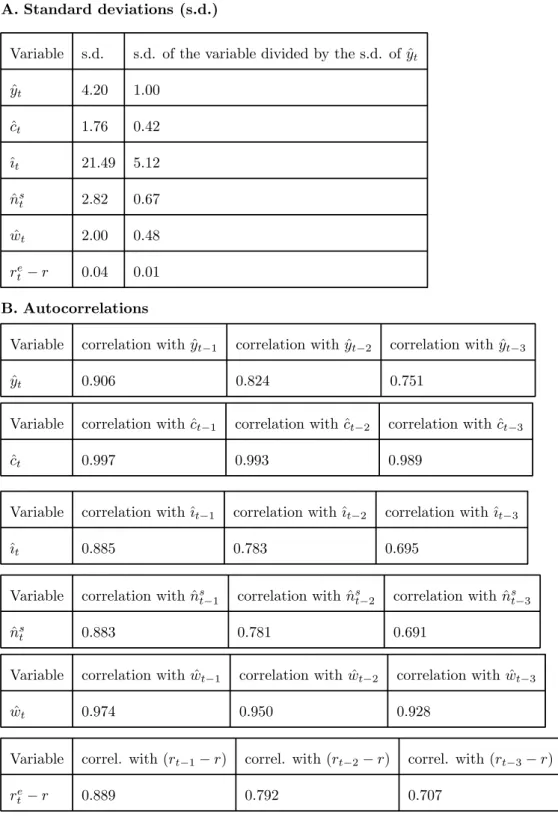
We can do this for 10000 periods and then summarize the statistical properties of the series we obtained for the various variables ˆyt, ˆct, ˆıt, ˆnst, ˆwt, ...
Table 1. Stochastic simulation. Shocks in the firms’ technological parameter. A. Standard deviations (s.d.)
Variable s.d. s.d. of the variable divided by the s.d. of ˆyt
ˆ yt 4.20 1.00 ˆ ct 1.76 0.42 ˆıt 21.49 5.12 ˆ ns t 2.82 0.67 ˆ wt 2.00 0.48 re t − r 0.04 0.01 B. Autocorrelations
Variable correlation with ˆyt−1 correlation with ˆyt−2 correlation with ˆyt−3
ˆ
yt 0.906 0.824 0.751
Variable correlation with ˆct−1 correlation with ˆct−2 correlation with ˆct−3
ˆ
ct 0.997 0.993 0.989
Variable correlation with ˆıt−1 correlation with ˆıt−2 correlation with ˆıt−3
ˆıt 0.885 0.783 0.695
Variable correlation with ˆns
t−1 correlation with ˆnst−2 correlation with ˆnst−3
ˆ
nst 0.883 0.781 0.691
Variable correlation with ˆwt−1 correlation with ˆwt−2 correlation with ˆwt−3
ˆ
wt 0.974 0.950 0.928
Variable correl. with (rt−1− r) correl. with (rt−2− r) correl. with (rt−3− r)
re
t − r 0.889 0.792 0.707
Variable Correlation with ˆ yt−12 yˆt−8 yˆt−4 yˆt−2 yˆt−1 yˆt yˆt+1 yˆt+2 yˆt+4 yˆt+8 yˆt+12 ˆ yt 0.35 0.49 0.69 0.82 0.91 1.00 0.91 0.82 0.69 0.49 0.35 ˆ ct 0.64 0.64 0.61 0.59 0.58 0.56 0.51 0.47 0.41 0.30 0.23 ˆıt 0.15 0.31 0.55 0.72 0.82 0.94 0.85 0.77 0.64 0.45 0.32 ˆ ns t 0.10 0.27 0.51 0.69 0.79 0.91 0.82 0.74 0.61 0.43 0.30 ˆ wt 0.60 0.65 0.72 0.76 0.79 0.81 0.74 0.68 0.57 0.42 0.31 re t − r -0.07 0.10 0.35 0.53 0.64 0.77 0.69 0.62 0.51 0.35 0.24 In these tables, (re
t− r) denotes the deviation of the ex-ante real interest rate from its
steady-state value.
We may summarize as follows the main results obtained in table 1 and in figures 1 to 8. First: consumption, investment and “labour effort” are procyclical. Second: consumption is less volatile than output and investment is more volatile than output. These are very well documented stylized facts about the United States economy [ references on this include Kydland and Prescott (1990) and Backus and Kehoe (1992)].
Our pattern of results is similar to the one obtained by King, Plosser and Rebelo (1988). The reason why our results are not exactly the same as those obtained by King, Plosser and Rebelo has to do both with the fact that ours is a zero growth version of their model and with the fact that our calibration is slightly different. For example, in our calibration the investment share of output was set at 0.167 whereas King, Plosser and Rebelo use the value 0.295 (their value probably results from including expenditure on consumer durables in the total amount of investment expenditure).
13
Conclusion
We have presented a detailed derivation of the competitive equilibrium of an economy. We have used a decentralized way of obtaining this equilibrium and have specified all the assumptions involved. Our method makes clear how each of these assumptions could be replaced by a different one and still let us proceed with the derivation of the general equilibrium without much difficulty.
Although we have arrived at the same set of equations as King, Plosser and Rebelo (1988) - who use a central planner’s approach - our method has the advantage that it can be used in many situations where the second welfare theorem does not hold.
It results obvious that we are able to generate the same key business cycle facts that King, Plosser and Rebelo are able to generate with their model: (i) consumption, investment and work hours are procyclical; (ii) consumption is less volatile than real output whereas investment is more volatile than real output.
Appendix
In this appendix, we derive in an intuitive way the first order conditions of the firms’ problem and the first order conditions of the households’ problem. Let us start with the firms’ problem.
The first order condition in terms of the choice of labour demand can be obtained as follows. The expected marginal benefit of increasing ndt0+j by one unit is the increased output that will be obtained. This is given by the marginal product of labour, Ato+jF2
¡ kt0+j,n d t0+j ¢ . Discounting this to period t0, we have
Ato+jF2 ¡ kt0+j,n d t0+j ¢ (1 + rt0)...(1 + rt0−1+j)
Since the firm is in period t0 when it is making these decisions, it must think in terms of
Et0 " Ato+jF2 ¡ kt0+j,n d t0+j ¢ (1 + rt0)...(1 + rt0−1+j) #
The expected marginal cost of increasing nd
t0+j by one unit is the wage payment that it implies, wt0+j. Discounting this amount to period t0, we have
wt0+j
(1 + rt0)...(1 + rt0−1+j)
Since the firm is in period t0 when it is making these decisions, it must think in terms of
Et0 ∙
wt0+j
(1 + rt0)...(1 + rt0−1+j) ¸
The optimal choice of nd
t0+j is the point where expected marginal benefit is equal to expected marginal cost. Therefore, the condition is
Et0 " Ato+jF2 ¡ kt0+j,n d t0+j ¢ (1 + rt0)...(1 + rt0−1+j) # = Et0 ∙ wt0+j (1 + rt0)...(1 + rt0−1+j) ¸ (83)
Let us now try to obtain the first order condition in terms of the choice of capital. Note that in period (t0+ j) the household chooses kt0+1+j. kt0+j is pre-determined [it was determined in period (t0− 1 + j)].
The expected marginal benefit of increasing kt0+1+j by one unit is obtained as follows. If, in period (t0+ j), the firm decides to increase kt0+1+j by one unit, that extra unit of capital shall produce an increase in output in period (t0+ 1 + j) given by Ato+1+jF1
¡ kt0+1+j,n d t0+1+j ¢ . The use of capital in production involves depreciation so that, after production, all that is left of that extra unit of capital is (1−δ) units of capital [or (1−δ) units of output since units of capital in this model correspond to units of output]. Therefore, the overall benefit of increasing kt0+1+j in period (t0+j) by one unit is that in period (t0+1+j) the firm will obtain
£ Ato+1+jF1 ¡ kt0+1+j,n d t0+1+j ¢ + (1 − δ)¤ units of output. Discounting this amount to period t0, we obtain
Ato+1+jF1 ¡ kt0+1+j,n d t0+1+j ¢ + (1 − δ) (1 + rt0)...(1 + rt0−1+j)(1 + rt0+j)
Since the firm is in period t0 when it is making these decisions, it must think in terms of
Et0 " Ato+1+jF1 ¡ kt0+1+j,n d t0+1+j ¢ + (1 − δ) (1 + rt0)...(1 + rt0−1+j)(1 + rt0+j) #
The expected marginal cost of increasing kt0+1+j by one unit is the reduction in the amount of dividends paid in period (t0+ j). This reduction in real terms corresponds to one unit of output:
the one unit of output that is used for investment. Discounting this amount to period t0, we have
1
(1 + rt0)...(1 + rt0−1+j)
Since the firm is in period t0 when it is making these decisions, it must think in terms of
Et0 ∙
1
(1 + rt0)...(1 + rt0−1+j) ¸
Hence, the first order condition in terms of the choice of capital is
Et0 " Ato+1+jF1 ¡ kt0+1+j,n d t0+1+j ¢ + (1 − δ) (1 + rt0)...(1 + rt0−1+j)(1 + rt0+j) # = = Et0 ∙ 1 (1 + rt0)...(1 + rt0−1+j) ¸ (84)
We start by defining λt0+j as the marginal utility of output in period (t0+ j). In other words, λt0+jgives us the increase/decrease in an household’s utility that would follow an increase/decrease of one (infinitesimal) unit in the amount of output available to that household. This corresponds to the increase/decrease in the household’s utility that would be caused by consuming one more/less unit of output.
In short, λt0+j is defined as giving us the marginal utility that the consumer would obtain if he/she were given an extra unit of output to consume. Mathematically, then, we can write
λt0+j= u1(ct0+j, 1 − n
s t0+j)
Applying the expectations operator to both sides of this equation we obtain
Et0[λt0+j] = Et0 £ u1(ct0+j, 1 − n s t0+j) ¤ (85)
Let us now look at the optimal choice of ns t0+j. The expected marginal cost of increasing ns
t0+jby one unit is that this implies a reduction of one unit in the amount of leisure that the household enjoys during period (t0+j). The decrease in utility
that results from this is given by u2(ct0+j, t0+j) = u2(ct0+j, 1−n
s
t0+j). Since we are taking decisions at period t0, we have to use the expected value of this amount which is Et0
£ u2(ct0+j, 1 − n s t0+j) ¤ . The expected marginal benefit of increasing ns
t0+j by one unit is that we receive wt0+j units of output. In period (t0+ j) utility terms, the value of this is λt0+jwt0+j. Since the household is taking decisions at period t0, it has to think in terms of Et0[λt0+jwt0+j].
The first order condition on ns
t0+j is obtained by equating expected marginal cost to expected marginal benefit. Hence, the condition is
Et0 £ u2(ct0+j, 1 − n s t0+j) ¤ = Et0[λt0+jwt0+j] (86)
Let us now look at the optimal choice of bt0+1+j. Note that in period (t0+ j) the household chooses bt0+1+j. bt0+j is pre-determined [it was determined in period (t0− 1 + j)].
The expected marginal cost of increasing bt0+1+j[the amount of output paid to other households in period (t0+ 1 + j)] by one unit is the corresponding loss in utility. By having one less unit
of output in period (t0+ 1 + j), the household loses λt0+1+j in period (t0+ 1 + j) utility terms. Discounting this to period (t0+j) utility we obtain βλt0+1+j. Since plans are being made in period t0, the household has to think in terms of Et0[βλt0+1+j].
The expected marginal benefit of increasing bt0+1+j [the amount paid to other households in period (t0+ 1 + j)] by one unit is obtained as follows. If the household is going to pay one more
unit of output in period (t0+ 1 + j) it must be because it borrowed an extra (1+r1
t0+j) units of output in period (t0+ j). In period (t0+ j) utility terms, this is worth
λt0+j
(1+rt0+j). Since plans are being made in period t0, the household has to think in terms of Et0
h λ t0+j
(1+rt0+j) i
.
The first order condition on bt0+1+jis obtained by equating expected marginal cost to expected marginal benefit. Hence, the condition is
Et0 ∙ λt0+j (1 + rt0+j) ¸ = Et0[βλt0+1+j] (87)
Let us now look at the optimal choice of ztf0+1+j.
The expected marginal cost of increasing ztf0+1+j by one unit is obtained as follows. If the household decides to buy a fraction (1/v) of firm f in period (t0+ j), it will have to pay (1/v)qtf0+j. In period (t0+ j) utility terms, the value of this is λt0+j(1/v)q
f
t0+j. Since the household is at t0 when it is making these plans, it must think in terms of Et0
h λt0+j(1/v)q f t0+j i .
The expected marginal benefit of increasing ztf0+1+j by one unit is obtained as follows. If the household buys a fraction (1/v) of firm p in period (t0+ j), it will be entitled to a share in the
dividends in period (t0+ 1 + j) amounting to (1/v)πft0+1+j. In addition to this, the household will be able to sell this fraction (1/v) of firm p in period (t0+ 1 + j) thereby earning (1/v)qtf0+1+j. In period (t0+ 1 + j) utility terms the sum of the two amounts that the household receives is
worth λt0+1+j h
(1/v)πft0+1+j+ (1/v)qtf0+1+ji. In period (t0+ j) utility terms, the value of this
is βλt0+1+j h
(1/v)πft0+1+j+ (1/v)qtf0+1+ji. Since the household is at t0 when it is making these
plans, it must think in terms of Et0 h
βλt0+1+j h
(1/v)πft0+1+j+ (1/v)qft0+1+jii. Therefore, the condition is
Et0 h λt0+j(1/v)q f t0+j i = Et0 h βλt0+1+j h (1/v)πft0+1+j+ (1/v)qft0+1+jii or equivalently
Et0 h λt0+jq f t0+j i = Et0 h βλt0+1+j(π f t0+1+j+ q f t0+1+j) i (88)
When making its plans regarding present and future amounts of consumption, work effort, borrowing and shares, the household must also take into account the budget constraints that it will be facing in each period (present and future). The budget constraint for period (t0+ j) is
given by wt0+jn s t0+j+ bt0+1+j 1 + rt0+j + f =FX f =1 ztf0+jπft0+j = ct0+j+ bt0+j+ f =FX f =1 qtf0+j(ztf0+1+j− ztf0+j)
Since the household is at t0 when it is making its plans, it must think in terms of
Et0 ⎡ ⎣wt0+jn s t0+j+ bt0+1+j 1 + rt0+j + f =FX f =1 zft0+jπft0+j ⎤ ⎦ = = Et0 ⎡ ⎣ct0+j+ bt0+j+ f =FX f =1 qft0+j(zft0+1+j− zft0+j) ⎤ ⎦ (89)
References
[1] Backus, D. and Kehoe, P. 1992. International evidence on the historical properties of business cycles. American Economic Review 82: 864-888.
[2] Blanchard, O. and Khan, C. (1980). The solution of linear difference models under rational expectations. Econometrica 48: 1305-1311.
[3] Hansen, G. 1985. Indivisible labor and the business cycle. Journal of Monetary Economics 56: 309-327.
[4] King, R., Plosser, C. and Rebelo, S. (1988). Production, growth and business cycles: I. The basic neoclassical model. Journal of Monetary Economics 21: 195-232.
[5] Kydland, F. and Prescott, E. (1982). Time to build and aggregate fluctuations. Econometrica 50: 1345-1370.
[6] Kydland, F. and Prescott, E. 1990. Business cycles: real facts and a monetary myth. Quarterly Review. Federal Reserve Bank of Minneapolis, Spring.