www.hydrol-earth-syst-sci.net/20/4867/2016/ doi:10.5194/hess-20-4867-2016
© Author(s) 2016. CC Attribution 3.0 License.
The Budyko functions under non-steady-state conditions
Roger Moussa1and Jean-Paul Lhomme2
1INRA, UMR LISAH, 2 place Viala, 34060 Montpellier, France 2IRD, UMR LISAH, 2 place Viala, 34060 Montpellier, France Correspondence to:Roger Moussa ([email protected])
Received: 22 July 2016 – Published in Hydrol. Earth Syst. Sci. Discuss.: 26 July 2016 Revised: 19 October 2016 – Accepted: 16 November 2016 – Published: 12 December 2016
Abstract.The Budyko functions relate the evaporation ratio
E / P (Eis evaporation andP precipitation) to the aridity in-dex8=Ep/ P(Epis potential evaporation) and are valid on long timescales under steady-state conditions. A new physi-cally based formulation (noted as Moussa–Lhomme, ML) is proposed to extend the Budyko framework under non-steady-state conditions taking into account the change in terrestrial water storage 1S. The variation in storage amount 1S is taken as negative when withdrawn from the area at stake and used for evaporation and positive otherwise, when removed from the precipitation and stored in the area. The ML formu-lation introduces a dimensionless parameterHE= −1S / Ep and can be applied with any Budyko function. It represents a generic framework, easy to use at various time steps (year, season or month), with the only data required beingEp,P
and1S. For the particular case where the Fu–Zhang equa-tion is used, the ML formulaequa-tion with 1S≤0 is similar to the analytical solution of Greve et al. (2016) in the standard Budyko space (Ep/ P,E / P), a simple relationship existing between their respective parameters. The ML formulation is extended to the space [Ep/(P−1S), E /(P−1S)] and compared to the formulations of Chen et al. (2013) and Du et al. (2016). The ML (or Greve et al., 2016) feasible domain has a similar upper limit to that of Chen et al. (2013) and Du et al. (2016), but its lower boundary is different. Moreover, the domain of variation ofEp/(P−1S) differs: for1S≤0, it is bounded by an upper limit 1/ HE in the ML formula-tion, while it is only bounded by a lower limit in Chen et al.’s (2013) and Du et al.’s (2016) formulations. The ML for-mulation can also be conducted using the dimensionless pa-rameterHP= −1S / P instead ofHE, which yields another form of the equations.
1 Introduction
The Budyko framework has become a simple tool that is widely used within the hydrological community to estimate the evaporation ratioE / P at catchment scale (E is evap-oration andP precipitation) as a function of the aridity
in-dex8=Ep/ P (Epis potential evaporation) through simple mathematical formulations E / P=B1(8) and with long-term averages of the variables. Most of the formulations were empirically obtained (e.g., Oldekop, 1911; Turc, 1954; Tixe-ront, 1964; Budyko, 1974; Choudhury, 1999; Zhang et al., 2001; Zhou et al., 2015), but some of them were analyti-cally derived from simple physical assumptions (Table 1): (i) the one derived by Mezentsev (1955) and then by Yang et al. (2008), which has the same form as the one initially pro-posed by Turc (1954) (noted hereafter as Turc–Mezentsev); (ii) the one derived by Fu (1981) and reworked by Zhang et al. (2004) (noted hereafter as Fu–Zhang). These two last for-mulations involve a shape parameter (respectively,λandω), which varies with catchment characteristics and vegetation dynamics (Donohue et al., 2007; Yang et al., 2009; Li et al., 2013; Carmona et al., 2014). When its value increases, actual evaporation gets closer to its maximum rate.
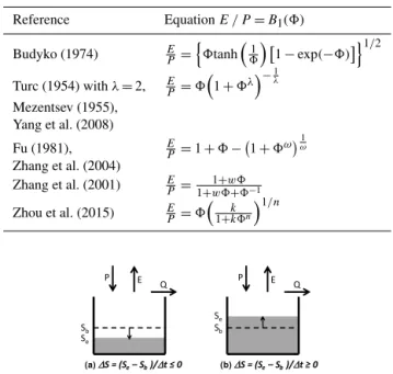
Table 1.Different expressions for the Budyko curves under steady-state conditions.
Reference EquationE / P=B1(8)
Budyko (1974) E P =
n
8tanh811
−exp(−8)o1/2
Turc (1954) withλ=2, E P =8
1+8λ−
1 λ
Mezentsev (1955), Yang et al. (2008)
Fu (1981), E
P =1+8− 1+8ω ω1 Zhang et al. (2004)
Zhang et al. (2001) E P =
1+w8
1+w8+8−1
Zhou et al. (2015) E P =8
k
1+k8n
1/n
P E Q
Se
Sb
P E Q
Se
Sb
(a)DS = (Se– Sb )/Dt 0 (b)DS = (Se– Sb )/Dt 0
Figure 1. Representation of the change in soil water storage
1S=(Se−Sb)/ 1t for the two cases considered in the paper:
1S≤0 and1S≥0.SbandSeare, respectively, the storage at the
beginning and the end of the time period1t.
and the month (Zhang et al., 2008; Du et al., 2016). How-ever, the water storage variation 1S cannot be considered
as negligible when dealing with these finer timescales or for unclosed basins (e.g., soil, groundwater, reservoir, snow, in-terbasin water transfer, irrigation; Jaramillo and Destouni, 2015). In these cases, the catchment is considered to be under non-steady-state conditions (Fig. 1) and the basin water bal-ance should be written asP=E+Q+1S. Table 2 shows some recent formulations of the Budyko framework extended to take into account the change in catchment water storage
1S. Chen et al. (2013) (used in Fang et al., 2016) and Du et al. (2016) proposed empirical modifications of the Turc– Mezentsev and Fu–Zhang equations, respectively, precipita-tionP being replaced by the available water supply defined as (P−1S), with Du et al. (2016) including the interbasin
water transfer into1S. Greve et al. (2016) analytically
mod-ified the Fu–Zhang equation in the standard Budyko space (Ep/ P,E / P) introducing an additional parameter, whereas Wang and Zhou (2016) proposed in the same Budyko space a formulation issued from the hydrological ABCD model (Al-ley, 1984), but with two additional parameters.
With the extension of the Budyko framework to non-steady-state conditions being a real challenge, this paper aims to propose a new formulation inferred from a clear physical rationale and compared to other non-steady formu-lations previously derived. The paper is organized as follows. First, we present the new formulation under non-steady-state conditions: its upper and lower limits, its generic equations
under restricted evaporation in the Budyko space (Ep/ P,
E / P) and in the space [Ep/(P−1S),E /(P−1S)]. Sec-ond, we compare the new formulation to the analytical solu-tion of Greve et al. (2016) in the standard Budyko space and to the formulations of Chen et al. (2013) and Du et al. (2016) in the space [Ep/(P−1S),E /(P−1S)].
2 New generic formulation under non-steady-state conditions
2.1 Upper and lower limits of the Budyko framework In the Budyko framework, each catchment is characterized by the three hydrologic variables (P,E andEp) which are represented in a 2-D space using dimensionless variables equal to the ratio between two of these variables and the third one. In the rest of the paper, following Andréassian et al. (2016), the space defined by (8=Ep/ P, E / P) is called Budyko space and the one defined by (8−1=P / Ep,
E / Ep) is called Turc space. For steady-state conditions (1S=0), it should be recalled that any Budyko functionB1 defined in the Budyko space (Ep/ P, E / P) generates an equivalent functionB2in the Turc space expressed as
E Ep =
B2
8−1=B1(8)
8 , (1)
and that any Budyko function verifies the following con-ditions under steady-state concon-ditions: (i) E=0 if P=0;
(ii) E≤P if P≤Ep (water limit); (iii) E≤Ep if P≥Ep (energy limit); (iv)E→EpifP→ ∞.
First, we present the upper and lower limits in the Turc space under steady-state conditions, when all the water con-sumed by evaporation comes from the precipitation, the change in water storage1Sbeing nil (E=P−Q). Figure 2a represents the variation of maximum and minimum actual evapotranspiration, respectively, Ex andEn, as a function
of precipitationP with dimensionless variables. The upper solid line represents the dimensionless maximum evapora-tion rateEx/ Ep: it follows the precipitation up toP / Ep=1 (the water limit is presented in bold blue on all graphs) and then is limited by potential evaporation Ex/ Ep=1 (the energy limit is in bold green). The lower solid line (in bold black) represents the dimensionless minimum evapo-ration rate En/ Ep which follows the x axis: En/ Ep=0. The feasible domain between the upper and the lower lim-its is shown in grey. In the Budyko space, we have the fol-lowing relationships: (i) when evaporation is maximum, for
Ep/ P≤1,Ex/ P=Ep/ P and forEp/ P≥1,Ex/ P=1;
(ii) when evaporation is minimum:En/ P=0. The
corre-sponding Budyko non-dimensional graph is shown in Fig. 2b and represents the upper and lower limits of the feasible do-main ofE / P=B1(Ep/ P).
Table 2.Different expressions for the Budyko curves under non-steady-state conditions.
Reference Steady-state conditions Non-steady-state conditions
B1(8)
Greve et al. (2016) Fu–Zhang E P =1+
Ep
P − h
1+(1−y0)κ−1EPpκi1/κwithκandy0parameters
Chen et al. (2013) Turc–Mezentsev E P−1S =
1+
Ep
P−1S−8t −λ−
1 λ
withλand8tparameters
Du et al. (2016) Fu–Zhang E
P−1S =1+ Ep
P−1S− h
1+
Ep
P−1S ω
+µ
iω1
withωandµparameters
0 1 2 3
0 1 2
-1 = P/E p
E/
Ep (a)
Energy limit E x/Ep = 1
Wat er lim
it
E/Ex p =
-1
E n/Ep = 0
0 1 2 3
0 1 2
= E
p/P
E/
P
(b)
Water limit E
x/P = 1
Ene rgy
lim it
E/Px
=
E n/P = 0
0 1 2 3
0 1 2
-1 = P/E p E/ Ep 1-H E H E (c) E x/Ep = 1
Ex/E p =
-1 + HE
E n/Ep = HE
0 1 2 3
0 1 2
(d)
= E
p/P E/ P 1/(1-H E) 1/(1-H E)
Ex/P = 1 + HE
En/P =
HE
E/Px
=
0 1 2 3
0 1 2
(e)
-1 = P/E p
E/
Ep
-H E 1-HE
E x/Ep = 1
E/Ex p =
-1 + HE
E n/Ep = 0
0 1 2 3
0 1 2
(f)
= E
p/P
E/
P
1/(1-H
E) -1/HE
1/(1-H
E) Ex/P = 1 + H
E
E n/P = 0
E/Px
= Budyk o ’s space T ur c’ s space
Steady-state conditions Non-steady-state conditions
S = 0 (HE= 0) S 0 (HE 0) S 0 (HE 0)
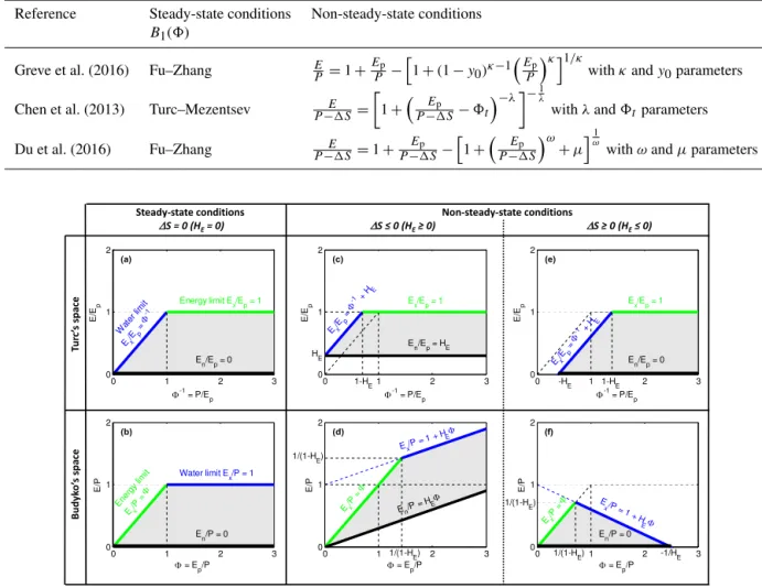
Figure 2.Upper and lower limits of the feasible domain (in grey) of evaporation in the Turc space (P / Ep,E / Ep) and in the Budyko space
(Ep/ P,E / P) (water limit in blue, energy limit in green and lower limit in black) when using the non-dimensional parameterHE: (aand b) for steady-state conditions; (c,d,eandf) for non-steady-state conditions with a storage term1S(canddfor1S≤0; and(e)and(f)for
1S≥0).
evaporation process (for instance, groundwater depletion for irrigation), or a given amount of the precipitation 1S is
stored in the area (soil water, ground water, reservoirs) fol-lowing the water balance (E=P−1S−Q). As shown in Fig. 1, the storage amount1Sis taken as negative (1S≤0) when withdrawn from the area and used for evaporation; it is taken as positive (1S≥0) when removed from the precip-itation and stored in the area. When 1S is negative,|1S|
should be lower than Ep because if |1S| ≥Ep, evapora-tion would be systematically equal toEp; when1S is pos-itive, it should be necessarily lower than P. Consequently,
−Ep≤1S≤P. The variable1Sis used in a dimensionless form, either as HE= −1S / Ep or HP= −1S / P, which are positive when additional water is available for evapotran-spiration and negative when water is withdrawn from precipi-tation. In the following, all the calculations are made withHE (−8−1≤HE≤1), but a similar reasoning is conducted using
HP (−1≤HP≤8) in Appendix A. Taking into account1S makes the upper and lower limits of the feasible domain dif-ferent.
In the Turc space, the case where evaporation is at its maxi-mum value is visualized as the upper limit in Fig. 2c and e (all the available water is used for evaporation). For both cases,
1S≤0 (Fig. 2c) or1S≥0 (Fig. 2e), we haveEx=P−1S
ifP−1S≤EP andEx=EP ifP−1S≥EP. Written with
dimensionless variables, these equations transform into
if P
Ep ≤1+
1S Ep then
Ex
Ep =
P Ep−
1S Ep =8
−1+H
E, (2) if P
Ep ≥1+
1S Ep then
Ex
Ep =1. (3)
For the minimal value of evapotranspiration En, we have
1S≥0 (Fig. 2e).
if1S≤0 then En
Ep
=−1S
Ep
=HE. (4a)
if1S ≥ 0 thenEn
Ep
=0 (4b)
Translating the above equations into the Budyko space (Fig. 2d, f) yields the following for the upper limits: if Ep
P ≥ Ep
Ep+1S then
Ex
P =1− 1S
P =1+HE Ep
P
=1+HE8, (5)
if Ep
P ≤ Ep
Ep+1S then
Ex
P =
Ep
P =8. (6)
Equation (5) has two limits: whenHE=0,Ex/ P=1, and
when1S→ −Ep, which corresponds toHE=1, Ex/ P →
(1+8). For the lower limits in the Budyko space we have if1S ≤ 0 thenEn
P =
−1S
P =HE Ep
P =HE8, (7a)
if1S ≥ 0 thenEn
P =0. (7b)
Note that under steady-state conditions, the upper and lower limits are similar in both Turc and Budyko spaces, while this is not the case under non-steady-state conditions. It is also interesting to note that for the negative values ofHEthe do-main of variation of8is bounded [0,−1/ HE] and the
pos-sible space of the Budyko functions is limited to a triangle (Fig. 2f).
2.2 General equations with restricted evaporation We now examine the case where the evaporation rate is lower than its maximum possible rate. In the Turc space, under non-steady-state conditions (1S≤0 in Fig. 2c or 1S≥0 in Fig. 2e), Eq. (1) should be transformed to take into ac-count the impact of water storage on the evaporation pro-cess. We search a mathematical formulation which trans-forms the upper and lower limits for the steady-state con-ditions (Fig. 2a) into the corresponding ones for the non-steady-state conditions (Fig. 2c if 1S≤0 and Fig. 2e if
1S≥0). The mathematical transformation is searched under
the formE / Ep=α B2(8−1+γ)+β, which combines an
x axis translation (γ), ayaxis translation (β) and a homoth-etic transformation (α). This mathematical form is suggested by the way the physical domain of Turc’s space is trans-formed when passing from steady-state conditions to non-steady-state conditions (Fig. 2a, c, e). Note that the reason-ing can be conducted either in the Turc or the Budyko space, but the upper and lower limits and the transformation from steady- to non-steady-state conditions are easier to grasp in the Turc space than in the Budyko space. We distinguish the two cases corresponding to1S≤0 and1S≥0.
2.2.1 Case1S≤0
In the Turc space, the lower limitB2(8−1)=0 in Fig. 2a transforms intoB2(8−1)=HE in Fig. 2c. Using the math-ematical transformation described above, we obtain (α×0)
+β=HE. Following a similar reasoning, the energy limit
B2(8−1)=1 transforms intoB2(8−1)=1, which yieldsα
+β=1, and the water limitB2(8−1)=8−1transforms into
B2(8−1)=HE+8−1, which yieldsα(8−1+γ)+β=HE
+8−1. The resolution of these three equations givesα=1
− HE, β=HE and γ=8−1HE/(1−HE). Consequently, Eq. (1) should be transformed into
E Ep
=(1−HE) B2
8−1 1−HE
+HE. (8)
By introducing Eq. (1) into Eq. (8), we obtain the formulation in the Budyko space (Fig. 2d):
E
P =(1−HE) 8B2 8−1
1−HE
+HE8
=B1[(1−HE) 8]+HE8. (9)
The derivative of Eq. (9) is
d EP
d8 =(1−HE)
dB1[(1−HE) 8]
d8 +HE. (10)
Given thatdB1[(1−HE)8]
d8 =1 for8=0 and
dB1[(1−HE)8]
d8 =0
when 8→ ∞, the derivative d
E P
d8 (i.e., the slope of the
curve) is equal to 1 for8=0, and when8→ ∞, the deriva-tive tends toHE.
2.2.2 Case1S≥0
Following the same reasoning as above, the lower limit, the energy limit and the water limit ofB2(8−1) in the Turc space in Fig. 2a (respectively, 0, 1 and 8−1) transform,
respec-tively, into 0, 1, andHE +8−1 in Fig. 2e. We obtain, re-spectively, the following three equations: (α×0)+β=0,α
+β=1 andα(8−1+γ)+β=HE+8−1. The resolution givesα=1,β=0 andγ=HE. Consequently, Eq. (1) should be transformed into
E Ep
=B2
8−1+HE
. (11)
By introducing Eq. (1) into Eq. (11), we obtain the formula-tion in the Budyko space (Fig. 2f):
E
P =8B2
8−1+HE
=(1+HE8) B1
8
1+HE8
. (12)
The derivative of Eq. (12) is
d EP
d8 =HEB1
8
1+HE8
+(1+HE8) dhB1
8
1+HE8
i
0 1 2 3 4 5 0
1 2 3
Φ = Ep/P
E/P
H E→ − ∞
ω = 1, 1.5, ∞
0 1 2 3 4 5
0 1 2 3
Φ = Ep/P
E/P
H E = −0.25
ω→ ∞
ω→ ∞
ω = 1.5
ω = 1
0 1 2 3 4 5
0 1 2 3
Φ = Ep/P
E/P
H E = 0
ω→∞
ω→ ∞
ω = 1.5
ω = 1
0 1 2 3 4 5
0 1 2 3
Φ = Ep/P
E/P
HE = 0.25
ω→∞
ω→ ∞
ω = 1.5
ω = 1
0 1 2 3 4 5
0 1 2 3
Φ = Ep/P
E/P
HE = 0.5
ω→ ∞
ω→ ∞
ω = 1.5
ω = 1
0 1 2 3 4 5
0 1 2 3
Φ = Ep/P
E/P
HE = 1
ω = 1, 1.5, ∞
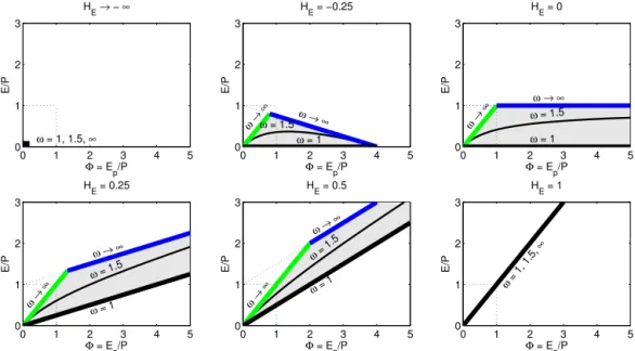
Figure 3.The ML formulation in the Budyko space with the Fu–Zhang relationship Eq. (14a, b) forω=1.5 and for different values ofHE.
The bold lines indicate the upper and lower limits of the feasible domain of evaporation (shown in grey).
Given that B1
8
1+HE8
=0 and d
h B1
8 1+HE8
i
d8 =1 for
8=0, the derivative d
E P
d8 is equal to 1 for 8=0. When
8→ −1/HE,B1
8
1+HE8
=1 and d h
B1
8 1+HE8
i
d8 =0, the
derivative d
E P
d8 tends toHE.
In the following, these new generic formulae (Eqs. 8 and 9 for1S≤0 and Eqs. 11 and 12 for1S≥0) are called ML formulations (ML stands for Moussa–Lhomme).
2.2.3 Application
Any Budyko equation B1(8) from Table 1 can be used in Eqs. (9) and (12) as detailed in Table S1 in the Supplement. It is worth noting that both the Turc–Mezentsev and Fu–Zhang functions, which are obtained from the resolution of a Pfaf-fian differential equation, have the following remarkable sim-ple property:F(1/ x)=F(x)/ x. This means that the same mathematical expression is valid for B1 and B2: B1=B2. Both Turc–Mezentsev and Fu–Zhang functions have similar shapes, and a simple linear relationship was established by Yang et al. (2008) between their parameters (see Table 1):
ω=λ+0.72. The ML formulation is used hereafter with the Fu–Zhang function (Table 1) for comparison with the ana-lytical solution of Greve et al. (2016) based upon the same function. Replacing B1by Fu–Zhang’s equation, in Eq. (9) for1S≤0 and in Eq. (12) for1S≥0, in the Budyko space,
gives
if1S ≤ 0 thenE
P =1+8−
1+(1−HE)ω8ω 1
ω, (14a)
if1S≥ 0 thenE
P =1+(1+HE) 8
−(1+HE8)ω+8ω
1
ω. (14b)
For8=0, and in both cases1S≤0 and 1S≥0, we have
E / P=0. However, the upper limits of8differ: for1S≤0, when8→ ∞,E / P→ ∞, while for1S≥0 the maximum value of8is−1/HEand corresponds toE / P=0. Figure 3
shows some examples of the shape of the ML formulation in the Budyko space (Eq. 14a, b) forω=1.5 and different val-ues ofHE. Note that for the particular and unlikely case when
HE→ −∞, upper and lower limits are reduced to the point (Ep/ P=0, E / P=0). For HE=0, we obtain the curves corresponding to steady-state conditions, while forHE=1, upper and lower limits are superimposed, and the domain is restricted to the 1 : 1 line. We can easily verify that all func-tions in Table S1 of the Supplement give similar results. 2.3 The ML formulation in the space [Ep/(P−1S),
E /(P−1S)]
As mentioned in the introduction, some authors (Chen et al., 2013; Du et al., 2016) have dealt with the non-steady condi-tions by modifying the Budyko reference space and replacing the precipitationPbyP−1S. Hereafter, we develop the ML
formulations in this new space. The upper limits of the ML formulations can be obtained by transforming Eqs. (5) and (6) defined in the Budyko space. We get, respectively, if Ep
P−1S ≥1 then Ex
P−1S =1, (15)
if Ep
P−1S <1 then Ex
P−1S = Ep
0 1 2 3 4 5 0
0.5 1
H E≤ 0
E p/(P−∆S)
E/(P−
∆
S)
ω→∞
ω →
∞
ω = 1.5
ω = 1
0 1 2 3 4 5
0 0.5 1
H
E = 0.25
E p/(P−∆S)
E/(P−
∆
S)
1/H E
ω→∞
ω →
∞ ω = 1.5
ω = 1
0 1 2 3 4 5
0 0.5 1
H E = 0.5
E p/(P−∆S)
E/(P−
∆
S)
1/H E ω → ∞
ω →
∞
ω = 1.5
ω = 1
0 1 2 3 4 5
0 0.5 1
H E = 1
E p/(P−∆S)
E/(P−
∆
S)
1/H E
ω = 1, 1.5, ∞
Figure 4.The ML formulation with the Fu–Zhang Eq. (21a, b) in the space [Ep/(P−1S),E /(P−1S)] forω=1.5 and four values of
HE. ForHE≥0, all curves have a common upper end at8′=1/ HEcorresponding toE /(P−1S)=1. The bold lines indicate the upper and lower limits of the feasible domain shown in grey. ForHE≤0, the curve is similar to the one under steady-state conditions.
The lower limits are obtained from Eq. (7a, b): if1S ≤ 0 then En
P−1S =
−1S
P−1S =HE Ep
P−1S, (17a)
if1S ≥ 0 then En
P−1S =0. (17b)
In the new space, we put
8′= Ep
P−1S = 8
1+HE8or
8= 8
′
1−HE8′
. (18)
Consequently, the relationship betweenE /(P−1S),8′and
E / P is given by
E
P−1S=
E P
P
P−1S =
1 1+HE8
E
P = 1−HE8
′E
P. (19)
Inserting Eqs. (9) and (12) into Eq. (19) and expressing8as a function of 8′ (Eq. 18) led to the ML formulation in the
new space:
if1S≤ 0 then E
P−1S
= 1
1+HE8
{B1[(1−HE) 8]+HE8}
= 1−HE8′B1
(1−H
E) 8′ 1−HE8′
+HE8′, (20a) if1S≥ 0 then E
P−1S =
1
1+HE8(1+HE8)
·B1
8
1+HE8
=B1 8′. (20b)
Note that for1S≥0,E /(P−1S)=B1(8′) is independent ofHE and is identical to the steady-state conditionHE=0. This is explained by the fact that the stored water 1S be-ing initially subtracted to the precipitation P, it does not participate in the evaporation process and consequently has no impact on the ratioE /(P−1S). For1S≤0, and for
8=0, i.e.,P→ ∞, we have 8′=0, B1=0 and E /(P−
1S)=0. When 8→ ∞, which corresponds to P→0, we
have8′=1/ HE,B1=1, andE /(P−1S)→1.
Any Budyko formulationB1in Table 1 can be used with Eq. (20a, b), as shown in Table S2 of the Supplement. When the Fu–Zhang equation is used, Eq. (20a, b) become
if1S≤0 then E
P−1S =1+(1−HE) 8 ′
− 1−HE8′ω+(1−HE)ω 8′ω1/ω, (21a)
if1S≥0 then E
P−1S =1+8
′− 1+8′ω1ω
. (21b)
Figure 4 shows the ML formulation (Eq. 21a, b) in the space [Ep/(P−1S), E /(P−1S)] for ω=1.5 and dif-ferent values of HE. For HE=0, we retrieve the original Fu–Zhang equation and when ω=1, we can easily verify that Eq. (21a, b) are equal to the lower limit of the do-mainE /(P −1S)=HEEp/(P−1S) when1S≤0, and
2.4 The ML formulation using the dimensionless parameterHP
A mathematical development, similar to the one of Sect. 2.1, 2.2 and 2.3, is conducted in Appendix A using the di-mensionless parameter HP= −1S / P=HE8 (instead of
HE= −1S / EP) and yields another form of the ML
formu-lation. Equivalent mathematical representations are obtained for 1S≤0 and1S≥0 in the different spaces explored in
Sect. 2.1, 2.2 and 2.3. Figures S1, S2 and S3 in the Sup-plement obtained with the parameterHPcorrespond, respec-tively, to Figs. 2, 3 and 4 obtained withHE. Similarly,
Ta-bles S3 and S4 in the Supplement (obtained withHP) cor-respond to Tables S1 and S2 in the Supplement (obtained withHE): they give the ML formulation applied to the differ-ent Budyko curves of Table 1 in the standard Budyko space (Ep/ P,E / P) and in the space [Ep/(P−1S),E /(P−
1S)]. Significant differences appear concerning the mathe-matical equations and the shape of the feasible domain de-fined by its upper and lower limits. This is due to the fact that usingHEorHPcorresponds to different sets of data and different functional representations. Both approaches (HEor
HP) can be used. When storage water contributes to enhanc-ing evaporation (1S≤0),1Sis bounded by potential
evapo-rationEP and consequently represents a given percentage of
EP. Hence, it is more convenient to useHE= −1S / Ep in-stead ofHP= −1S / P, becauseHElies in the range[0,1]
which is not the case forHP. Conversely, when precipitation water contributes to increase soil water storage (1S≥0),1S
is bounded byP and represents a percentage of precipitation
P. Consequently, usingHP is more convenient becauseHP lies in the range[−1,0]. Moreover, in order to keep the pa-rameter in the range[0,1],HP′ = −HPcould be preferred.
3 Comparing the new formulation with other formulae from the literature
3.1 In the standard Budyko space (Ep/ P,E / P)
When evapotranspiration exceeds precipitation (correspond-ing herein to the case 1S≤0), Greve et al. (2016) ana-lytically developed a Budyko-type equation where the wa-ter storage is taken into account through a paramewa-ter y0 (0≤y0≤1) introduced into the Fu–Zhang formulation (Ta-ble 2). In the Budyko space, this equation is written (Greve et al., 2016; Eq. 9) as
E
P =1+8− h
1+(1−y0)κ−18κ
i1/κ
. (22)
They used the shape parameterκto avoid confusion with the traditionalωof Fu–Zhang equation. Despite different phys-ical and mathematphys-ical backgrounds, Eqs. (14a) and (22) are exactly identical and a simple relationship betweenHEand
y0can be easily obtained. Equating Eqs. (14a) and (22) with
0 0.25 0.5 0.75 1
0 0.25 0.5 0.75 1
y 0 HE
ω = 1.1 ω = 1.5 ω = 2 ω = 5 ω
→ ∞
Figure 5.Relationship (Eq. 23) between the parameterHEof the
ML formulation (Eq. 14a) and the parametery0of the Greve et
al. (2016) (Eq. 22) for different values ofωwithω=κ.
0 1 2 3 4 5
0 1 2 3
y0 = 0 or HE = 0 y0 = 0.2 or
HE = 0.106 y0 = 0.
4 or HE = 0. 225 y0 = 0
.6 or HE = 0.36
7 y0 = 0
.8 or H
E =
0.553
y0 = 1 or
HE = 1
= E
p/P
E/
P
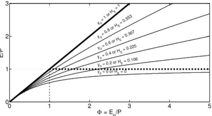
Figure 6.Example showing the similarity of the ML formulation Eq. (14a) and the equation of Greve et al. (2016) Eq. (22) (with
ω=κ=2) for different values ofy0; the corresponding values of
HEare calculated using Eq. (23).
ω=κ yields HE=1−(1−y0)
ω−1
ω . (23)
The relationship betweeny0andHEis independent from8. It is shown in Fig. 5 for different values ofω. For a given value of ω, we have HE<y0. For ω=1, we haveHE=0, and whenω→ ∞, we haveHE=y0.
The derivative of Eq. (22) gives
d EP
d8 =1−(1−y0)
κ−18κ−1h
1+(1−y0)κ−18κ i1−κκ
. (24)
For8=0, the derivative is equal to 1, and when8→ ∞, the
derivative tends to a value noted asmby Greve et al. (2016;
Eq. 12):
m=1−(1−y0) κ−1
κ . (25)
(assuming ω=κ). Greve et al. (2016; Sect. 4) show thaty0 is the maximum value of mreached whenω→ ∞. Hence, substituting in Eq. (22)y0by its value inferred from Eq. (23) yields an equation identical to that obtained from the ML formulation (Eq. 14a).
Figure 6 compares the ML formulation Eq. (14a) with Greve et al.’s (2016) analytical solution Eq. (22) for
ω=κ=2 and different values ofy0(0, 0.2, 0.4, 0.6, 0.8 and 1). The corresponding values ofHE(respectively, 0, 0.106, 0.225, 0.367, 0.553 and 1) are calculated using Eq. (23). The new ML formulation withω=κ, and only for1S≤0, gives exactly the same curves as those obtained by Greve et al. (2016). Both formulations are identical and have the same upper and lower limits. Greve et al. (2016), however, did not mention the lower limit and limited the reasoning to positive values ofy0. Moreover, the case of1S≥0 is not considered
by Greve et al. (2016).
3.2 In the space [Ep/(P−1S),E /(P−1S)]
The formulations proposed by Chen et al. (2013) and Du et al. (2016) in the space[Ep/ (P−1S), (E / (P−1S)]are es-sentially empirical. The Chen et al. (2013) function (Table 2) is derived from the Turc–Mezentsev equation and written as
E P−1S =
"
1+
E
p
P−1S−8t −λ#−
1 λ
. (26)
An additional parameter8t is empirically introduced in
or-der “to characterize the possible non-zero lower bound of the seasonal aridity index”; this parameter causes a shift of the curveE /(P−1S) along the horizontal axis such as for
Ep/ (P−1S)=8t, we haveE /(P−1S)=0. The
deriva-tive of Eq. (26) whenEp/(P−1S)→ ∞is equal to 0. Sim-ilarly, the Du et al. (2016) function (Table 2) is an empirical modification of Fu–Zhang equation (Fu, 1981; Zhang et al., 2004) written as
E
P−1S =1+ Ep
P−1S−
1+
E
p
P−1S ω
+µ
1ω . (27)
A supplementary parameter, noted here asµ(>−1), is added to modify the lower bound of the aridity index EP /(P−
1S). The parameterµplays a similar role as8t in Eq. (26).
For µ=0, Eq. (27) takes the original form of Fu–Zhang equation, (P−1S) replacingP. Whenµbecomes positive, the lower end of the curveE /(P−1S) shifts to the right. The functionE /(P−1S) in Eq. (27) is equal to zero for the
particular value ofEp/(P−1S)=8d, such as
(1+8d)ω=1+(8d)ω+µ. (28)
Greve et al.’s (2016) formulation can be also written in the space [Ep/(P−1S),E /(P−1S)]. Inserting Eq. (22) into Eq. (20a) and expressing8as a function of8′(Eq. 18) leads
0 1 2 3 4 5
0 0.5 1
ML, Greve et al. Chen et al.
Du et al.
Φ’ = E p/(P−∆S)
E/(P−
∆
S)
1/H E Φt , Φd
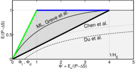
Figure 7.In the space [Ep/(P−1S),E /(P−1S)], an example comparing the three formulations: Du et al. (2016) withω=1.5 and 8d=0.5; Chen et al. (2013) with λ=ω−0.72=0.78 and 8t=8d=0.5; the ML formulation for 1S≤0 (Eq. 14a) with ω=1.5 andHE=0.25 (identical to Greve et al. 2016 formulation). The feasible domain of the ML formulation in dark grey is super-imposed over the domains of both Chen et al. (2013) and Du et al. (2016) in light grey.
to
E
P −1S =1+(1−HE) 8 ′−
1−HE8′κ
+(1−y0)κ−1 8′κi1/κ
. (29)
It can be mathematically shown that expressing (1−y0) in Eq. (29) as a function ofHEby inverting Eq. (23) (assum-ingω=κ) leads to the exact ML formulation of Eq. (21a). It is a direct consequence of the similarity of both formula-tions. Therefore, similar curves to those shown in Fig. 4 for the ML formulation withHE≥0 are obtained with Greve et al.’s (2016) formulation.
For1S≥0 (corresponding toHE≤0; Fig. 4), the three formulations (Chen et al.’s, 2013, Du et al.’s 2016, and ML) have similar upper and lower limits. For 1S≤0,
Fig. 7 shows an example of the curves obtained with Du et al.’s (2016) equation (ω=1.5) and Chen et al.’s (2013) equation with λ=0.78 (such as λ=ω−0.72 from Yang et al., 2008) and with 8t=8d=0.5 (corresponding to
µ=0.484 from Eq. 28). Both Chen et al.’s (2013) and Du et al.’s (2016) formulations are compared to the ML formu-lation using the Fu–Zhang Eq. (14a) withHE= +0.25. The ML and Greve et al. (2016) formulations are exactly identi-cal ifκ=ω=1.5 andy0=0.578 calculated from Eq. (23) for HE= +0.25. The four formulations have similar up-per limits but the lower limits are different. Both Chen et al.’s (2013) and Du et al.’s (2016) formulations have the
x axis as the lower limit andE /(P−1S) tends to 1 when 8′=Ep/(P−1S)→ ∞, while in the ML formulation with
1S≤0 (Fig. 2a) the feasible domain is a triangle, the domain
of variation of8′being limited by 0 and 1/ HE. 3.3 Discussion
the shape of the curve and another for its shift due to non-steady conditions:ωandHEfor the ML formulation (with the Fu–Zhang function),κ andy0for Greve et al. (2016),λ and8t for Chen et al. (2013),ωandµfor Du et al. (2016).
IfHE=y0=8t=µ=0, the four formulations are identical.
For1S≤0, the ML formulation with the Fu–Zhang equation (Eq. 14a) is identical to the one of Greve et al. (2016) in the Budyko space and also in the [Ep/(P−1S),E /(P−1S)] space, provided the shape parameters are assumed to be iden-tical (ω=κ) (a simple relationship is established betweenHE and the corresponding parametery0). Despite similar upper limits, the ML and Greve et al. (2016) formulations behave very differently from those of Chen et al. (2013) and Du et al. (2016) in the space [Ep/(P−1S),E /(P−1S)]. The ML formulation is different for1S≤0 and 1S≥0, while
those of Chen et al.’s (2013) and Du et al.’s (2016) do not dis-tinguish the two cases1S≤0 and1S≥0. All the formula-tions have the same upper limits, but the domain of variation of 8′ differs: respectively, [0, 1/ HE] when1S≤0 and [0,
∞] when1S≥0 for the ML formulation,[8t,∞]for Chen
et al. (2013) and[8d,∞]for Du et al. (2016) The lower end
of the curve E /(P −1S) corresponds, respectively, to (0, 0), (8t, 0) and (8d, 0) and the upper end to (1/ HE, 1) when
1S≤0 and (∞, 1) when1S≥0 for the ML formulation, (∞, 1) for the other two. Moreover, the ML formulation for
1S≥0 is reduced to a simple relationshipE /(P−1S)=B1 (8′) and is independent ofHE.
It is worth noting that for 1S≤0 the limits of Chen et
al. (2013) and Du et al. (2016) functions are not completely sound from a strict physical standpoint: for very high precip-itation, whenP≫Ep,8and8′should logically tend to zero and not to8tand8d; similarly, whenP→0, i.e.,8→ ∞, it
is physically logical that8′→Ep/(−1S)=1/ HE, as pre-dicted by our Eq. (20a). This tends to prove that the ML formulation, corroborated by the Greve et al. (2016) for-mulation, is physically more correct. Additionally, at simple glimpse, we note that the ML curves could be easily adjusted to the set of experimental points shown in Chen et al. (2013; Figs. 2 and 9) and in Du et al. (2016; Figs. 8 and 9).
4 Conclusion
The ML formulations constitute a general mathematical framework which allows any standard Budyko function de-veloped at catchment scale under steady-state conditions (Ta-ble 1) to be extended to non-steady conditions (Ta(Ta-ble S1 in the Supplement). They take into account the change in catch-ment water storage1S through a dimensionless parameter
HE= −1S / Epand the formulation differs according to the sign of1S(Eqs. 8 and 9 for1S≤0 and Eqs. 11 and 12 for
1S≥0). Applications can be conducted at various time steps (yearly, seasonal or monthly) both in the Turc space (P / Ep,
E / Ep) and in the standard Budyko space (Ep/ P,E / P), with the only data required to obtainEbeingEp,P and1S. The new formulations are inferred from an evaluation of the feasible domain of evaporation in the Turc space, ad-justed for the case where additional (1S≤0) or restricted (1S≥0) water is available for evaporation, and then trans-formed in the Budyko space. For 1S=0, the ML formu-lations return the original equations under steady-state con-ditions, with similar upper and lower limits in both spaces. Under non-steady-state conditions, however, the upper and lower limits of the feasible domain differ when using ei-ther the Turc or the Budyko space. The ML formulations can be extended to the [Ep/(P−1S),E /(P−1S)] space (Eq. 20a, b, Fig. 4). They can also be conducted using the dimensionless parameterHP= −1S / P instead ofHE, which yields another form of the equations (Appendix A and the Supplement). It is shown that the ML formulation with1S≤0 is identical to the analytical solution of Greve
et al. (2016) in the standard Budyko space, a simple rela-tionship existing between their respective parameters. On the other hand, the new formulation differs from those of Chen et al. (2013) and Du et al. (2016) in the space [Ep/(P−1S),
Appendix A: Scaling1SbyP instead ofEp
Appendix A presents the set of equations when scal-ing the change in soil water storage 1S by pre-cipitation P instead of potential evaporation Ep, i.e., using HP= −1S / P=HE8 (−1≤HP≤8) instead of
HE= −1S / Ep(−8−1≤HE≤1).
A1 Upper and lower limits of the Budyko framework In the Turc space, the upper limits of evapotranspiration
Ex/ Epare obtained from Eqs. (2) and (3): if P
Ep
≤1+1S
Ep then
Ex
Ep
= P
Ep
−1S
Ep
=(1+HP) 8−1, (A1) if P
Ep
≥1+1S
Ep then
Ex
Ep
=1, (A2)
and the lower limits of evapotranspiration En/ Ep from Eq. (4a, b):
if1S ≤ 0 thenEn
Ep
= −1S
Ep
=HP8−1, (A3a)
if1S ≥ 0 thenEn
Ep
=0. (A3b)
The translation in the Budyko space yields the following for the upper limits:
if Ep
P ≥ Ep
Ep+1S then
Ex
P =1− 1S
P =1+HP, (A4)
if Ep
P ≤ Ep
Ep+1S then
Ex
P =
Ep
P =8, (A5)
and the following for the lower limits: if1S≤ 0 thenEn
P = − 1S
P =HE Ep
P
=HE8=HP, (A6a)
if1S ≥ 0 thenEn
P =0. (A6b)
In the Supplement, Fig. S1 shows the upper and lower lim-its of the feasible domain of evaporation in the Turc and Budyko spaces, drawn with the parameter HP= −1S / P. Figure S1 in the Supplement corresponds to Fig. 2 obtained withHE= −1S / Ep.
A2 General equations with restricted evaporation We distinguish two cases:1S≤0 and1S≥0. Substituting
HE byHP/ 8in Eqs. (8), (9), (11) and (12) we obtain (if
1S≤0 in the Turc space)
E Ep
=1−HP8−1
B2
8−1 1−HP8−1
+HP8−1, (A7)
then in the Budyko space
E
P =B1(8−HP)+HP. (A8)
If1S≥0 in the Turc space
E Ep =B2
h
(1+HP) 8−1
i
, (A9)
then in the Budyko space
E
P =(1+HP) B1
8
1+HP
. (A10)
Replacing B1 by Fu–Zhang’s equation, in Eq. (A8) for
1S≤0 and in Eq. (A10) for1S≥0, gives the following in the Budyko space:
if1S≤0 then E
P =1+8−
1
+(8−HP)ωω1
, (A11a)
if1S≥0 then E
P =1+8+HP−
(1+HP)ω+8ω 1
ω. (A11b)
In the Supplement, Fig. S2 shows an example of the ML for-mulation (Eq. A11a, b) in the Budyko space obtained with the parameterHP= −1S / P. It corresponds to Fig. 3 ob-tained withHE= −1S / Ep. Table S3 gives the ML formu-lation applied to the different Budyko curves of Table 1 with the parameterHP(Eqs. A8 and A10). It corresponds to Ta-ble S1 in the Supplement obtained withHE.
A3 The ML formulation in the space [Ep/(P−1S),
E /(P−1S)]
Equations (15), (16), (17a) and (17b) yield the following for the upper limits:
if Ep
P−1S ≥1 then Ex
P−1S =1, (A12)
if Ep
P−1S ≤1 then Ex
P−1S = Ep
P−1S, (A13)
and the following for the lower limits: if1S≤ 0 then En
P−1S =
−1S
P −1S
=HE Ep
P−1S = HP
HP+1
, (A14a)
if1S ≥ 0 then En
P−1S =0. (A14b)
In the new space,[Ep/ (P−1S),E /(P−1S)], we put
8′= Ep
P −1S = 8
1+HP or
8=(1+HP) 8′. (A15) Consequently, the relationship between E /(P−1S) and E / P is given by
E P −1S =
E P
P P−1S =
1 1+Hp
E
ReplacingHEbyHP/ 8in Eq. (20a, b) we obtain if1S≤ 0 then E
P−1S =
1
1+HP[B1(8−HP)+HP]
= 1
1+HPB1
(1+HP) 8′−HP+ HP
1+HP, (A17a) if1S≥ 0 then E
P−1S =
1
1+HP
·(1+HP) B1
8
1+HP
=B1 8′. (A17b) Using the Fu–Zhang equation forB1we get
if1S≤ 0 then E
P−1S =1+8
′− HP 1+HP
−
1
1+HP
ω
+
8′− HP
1+HP
ω1/ω
, (A18a)
if1S ≥ 0 then E
P−1S =1+8
′− 1+8′ωω1
. (A18b) In the Supplement, Fig. S3 shows an example of the ML for-mulation (Eq. A18a, b) in the space [Ep/(P−1S),E /(P−
1S)] obtained with the parameterHP = −1S / P. It corre-sponds to Fig. 4 obtained withHE= −1S / Ep. Table S4 in the Supplement gives the ML formulation applied to the dif-ferent Budyko curves of Table 1 in the space [Ep/(P−1S),
Appendix B: List of symbols
B1(8) Relationship betweenE / P and8in the Budyko space (Ep/ P,E / P) such asE / P=B1(8) [–] B2(8−1) Relationship betweenE / Epand8−1=P / Epin the Turc space (P / Ep,E / Ep) such as
E / Ep=B2(8−1) [–] E actual evaporation [LT−1]
En Lower limit of the feasible domain of evaporation [LT−1]
Ep Potential evaporation [LT−1]
Ex Upper limit of the feasible domain of evaporation [LT−1]
HE −1S / Ep(−P / Ep≤HE≤1) [–]
HP −1S / P (−1≤HP≤Ep/ P) [–]
m Slope of the equation of Greve et al. (2016) when8→ ∞[–]
ML New formulations: Eqs. (8) and (9) for1S≤0 and Eqs. (11) and (12) for1S≥0 (stands for Moussa–Lhomme)
P Precipitation [LT−1] Q Runoff [LT−1]
y0 Parameter in the Greve et al. (2016) equation accounting for non-steady-state conditions (0≤y0≤1) [–]
κ Shape parameter in the Greve et al. (2016) equation corresponding toωin the Fu–Zhang equation [–]
1S Water storage variation [LT−1]
λ Shape parameter in the Turc–Mezentsev equation (λ> 0) [–] µ Parameter in the Du et al. (2013) equation [–]
8 Aridity index (8=Ep/ P) [–]
8d Aridity index threshold in the Du et al. (2016) equation corresponding toE /(P−1S)=0 [–]
8t Aridity index threshold in the Chen et al. (2013) equation [–]
8′ Ep/ (P−1S)[–]
The Supplement related to this article is available online at doi:10.5194/hess-20-4867-2016-supplement.
Acknowledgements. The authors are very grateful to the reviewers,
L. Gudmundsson and F. Jaramillo, and to the editor, M. Coenders-Gerrits, for their constructive comments of the manuscript. They also gratefully acknowledge the scientific and financial support of the UMR LISAH, as well as the always inspiring advice of A. Gaby.
Edited by: M. Coenders-Gerrits
Reviewed by: L. Gudmundsson and one anonymous referee
References
Alley, W. M.: On the treatment of evapotranspiration, soil moisture accounting, and aquifer recharge in monthly water balance mod-els, Water Resour. Res., 20, 1137–1149, 1984.
Andréassian, V., Mander, Ü., and Pae, T.: The Budyko hypothe-sis before Budyko: The hydrological legacy of Evald Oldekop, J. Hydrol., 535, 386–391, doi:10.1016/j.jhydrol.2016.02.002, 2016.
Budyko, M. I.: Climate and life, Academic Press, Orlando, FL, 508 pp., 1974.
Carmona, A., Sivapalan, M., Yaeger, M. A., and Poveda, G.: Re-gional patterns of interannual variability of catchment water bal-ances across the continental U.S.: A Budyko framework, Wa-ter Resour. Res., 50, 9177–9193, doi:10.1002/2014WR016013, 2014.
Chen, X., Alimohammadi, N., and Wang, D.: Modeling interannual variability of seasonal evaporation and storage change based on the extended Budyko framework, Water Resour. Res., 49, 6067– 6078, doi:10.1002/wrcr.20493, 2013.
Choudhury, B.: Evaluation of an empirical equation for annual evaporation using field observations and results from a biophys-ical model, J. Hydrol., 216, 99–110, 1999.
Donohue, R. J., Roderick, M. L., and McVicar, T. R.: On the impor-tance of including vegetation dynamics in Budyko’s hydrological model, Hydrol. Earth Syst. Sci., 11, 983–995, doi:10.5194/hess-11-983-2007, 2007.
Du, C., Sun, F., Yu, J., Liu, X., and Chen, Y.: New interpreta-tion of the role of water balance in an extended Budyko hy-pothesis in arid regions. Hydrol. Earth Syst. Sci., 20, 393–409, doi:10.5194/hess-20-393-2016, 2016.
Fang, K., Shen, C., Fisher, J. B., and Niu, J.: Improving Budyko curve-based estimates of long-term water partitioning using hy-drologic signatures from GRACE, Water Resour. Res., 52, 5537– 5554, doi:10.1002/2016WR018748, 2016.
Fu, B. P.: On the calculation of evaporation from land surface (in Chinese), Sci. Atmos. Sin., 5, 23–31, 1981.
Gentine, P., D’Odorico, P., Lintner, B. R., Sivandran, G., and Salvucci, G.: Interdependence of climate, soil, and vegetation as constrained by the Budyko curve, Water Resour. Res., 39, L19404, doi:10.1029/2012GL053492, 2012.
Greve, P., Gudmundsson, L., Orlowsky, B., and Seneviratne, S. I.: A two-parameter Budyko function to represent conditions under which evapotranspiration exceeds precipitation, Hydrol. Earth Syst. Sci., 20, 2195–2205, doi:10.5194/hess-20-2195-2016, 2016.
Istanbulluoglu, E., Wang, T., Wright, O. M., and Lenters, J. D.: In-terpretation of hydrologic trends from a water balance perspec-tive: The role of groundwater storage in the Budyko hypothesis, Water Resour. Res., 48, W00H16, doi:10.1029/2010WR010100, 2012.
Jaramillo, F. and Destouni, G.: Local flow regulation and irrigation raise global human water consumption and footprint, Science, 350, 1248–1250, 2015.
Li, D., Pan, M., Cong, Z., Zhang, L., and Wood, E.: Vegetation con-trol on water and energy balance within the Budyko framework, Water Resour. Res., 49, 969–976, doi:10.1002/wrcr.20107, 2013. Mezentsev, V.: More on the computation of total evaporation,
Me-teorol. Gidrol., 5, 24–26, 1955.
Oldekop, E. M.: On evaporation from the surface of river basins, Collection of the Works of Students of the Meteorological Obser-vatory, University of Tartu-Jurjew-Dorpat, Tartu, Estonia, p. 209, 1911.
Tixeront, J.: Prediction of streamflow, IAHS publication no. 63: General Assembly of Berkeley, IAHS, Gentbrugge, 118–126, 1964.
Turc, L.: Le bilan d’eau des sols: relations entre les précipitations, l’évaporation et l’écoulement, Ann. Agron., 5, 491–595, 1954. Wang, D.: Evaluating interannual water storage changes at
wa-tersheds in Illinois based on long-term soil moisture and groundwater level data, Water Resour. Res., 48, W03502, doi:10.1029/2011WR010759, 2012.
Wang, X.-S. and Zhou, Y.: Shift of annual water balance in the Budyko space for catchments with groundwater-dependent evapotranspiration, Hydrol. Earth Syst. Sci., 20, 3673–3690, doi:10.5194/hess-20-3673-2016, 2016.
Yang, D., Shao, W., Yeh, P. J. F., Yang, H., Kanae, S., and Oki, T.: Impact of vegetation coverage on regional water balance in the nonhumid regions of China, Water Resour. Res., 45, W00A14, doi:10.1029/2008WR006948, 2009.
Yang, H., Yang, D., Lei, Z., and Sun, F.: New analytical derivation of the mean annual water-energy balance equation, Water Re-sour. Res., 44, W03410, doi:10.1029/2007WR006135, 2008. Zhang, L., Dawes, W. R., and Walker, G. R.: Response of mean
an-nual evapotranspiration to vegetation changes at catchment scale, Water Resour. Res., 37, 701–708, 2001.
Zhang, L., Hickel, K., Dawes, W. R., Chiew, F. H. S., Western, A. W., and Briggs, P. R.: A rational function approach for esti-mating mean annual evapotranspiration, Water Resour. Res., 40, W02502, doi:10.1029/2003WR002710, 2004.
![Figure 4. The ML formulation with the Fu–Zhang Eq. (21a, b) in the space [E p / (P − 1S), E / (P − 1S)] for ω = 1.5 and four values of H E](https://thumb-eu.123doks.com/thumbv2/123dok_br/18410317.359694/6.918.244.678.100.466/figure-ml-formulation-fu-zhang-eq-space-values.webp)