REM WORKING PAPER SERIES
Optimal Tax Structure for Consumption and Income Inequality: an
Empirical Assessment
António Afonso, José Alves
REM Working Paper 051-2018
October 2018
REM – Research in Economics and Mathematics
Rua Miguel Lúpi 20, 1249-078 Lisboa,
Portugal
ISSN 2184-108X
Any opinions expressed are those of the authors and not those of REM. Short, up to two paragraphs can be cited provided that full credit is given to the authors.
Optimal Tax Structure for Consumption and Income
Inequality: an Empirical Assessment
*
Ant´
onio Afonso
, Jos´
e Alves
2018
Abstract
In the present empirical analysis, we try to assess the impact of taxation on investment growth. In particular, and by using gross fixed capital formation as a proxy for investment, we intend to evaluate the impact of the taxation structure in investment dynamics, in a short and a long-run perspectives. This empirical exercise was conducted for all OECD countries, during the 1980-2015 period. Through panel data econometric techniques, we find optimal tax-investment threshold values, especially higher for short-term than for long-term horizon. In addition, we find optimal income taxation around 9%, in percentage of GDP, an average optimal value of 12.7% for consumption taxes to promote annual investment growth.
Keywords: Investment Growth; Tax systems; Fiscal Policy; Optimal taxation JEL: D25; E62; H21; O47
*The opinions expressed herein are those of the authors and do not necessarily reflect those of their employers.
Any remaining errors are the author’s sole responsibility.
ISEG/UL - Universidade de Lisboa, Department of Economics; REM - Research in Economics and
Mathe-matics, UECE - Research Unit on Complexity and Economics. UECE is supported by FCT (Funda¸c˜ao para a Ciˆencia e a Tecnologia, Portugal). email: [email protected].
ISEG/UL - Universidade de Lisboa, Department of Economics; REM – Research in Economics and
Math-ematics, UECE – Research Unit on Complexity and Economics. UECE is supported by FCT (Funda¸c˜ao para a Ciˆencia e a Tecnologia, Portugal) Corresponding author: [email protected].
1
Introduction
The act to consume is the main purpose of economics. Yet, consumption is made essentially through economic markets, which can lead to several economic disruptions, namely, the non-inclusion of several externalities (positive and negative) and an inefficient income distribution of the financial resources spent.
In order to correct those disruptions, governments tend to use taxation as a key instrument. Several sources of taxation, such as on individual income and property, can lead to a reduction on income inequalities, as mentioned by Piketty (2014). Furthermore, some studies, as Mo (2000), Cingano (2014) and Ostry et al. (2014), highlight the positive linkage between income inequality reduction and economic performance.
Therefore, it is important to analyse the relationship between taxation structures and both consumption and income inequalities. The study of these two aspects allows to understand if fiscal policy indeed contributes to higher consumption and to lower inequalities, in what concerns the use of tax policies.
In our panel analysis for the period between 1980 and 2015, for OECD countries, we find some non-linear relationships between several tax items and the two above-mentioned variables, while uncovering also the respective optimizing thresholds.
The paper is structured as follows: section 2 reviews the literature regarding taxation effects on both consumption and income inequality; section 3 presents the methodology employed, as well as the data; section 4 reports and discusses the results; and lastly, section 5 provides our conclusions.
2
Literature Review
Taxing income may obviously have important consequences on consumption, income and wealth inequalities dynamics. As Piketty and Saez (2003) highlight, the existence of progressive income and estate tax systems for the United States case have prevented a rapid recovery of the wealth inequalities after the Great Depression and WWII.
In fact, and in what concerns the taxation effects on inequality, Saez (2004) concludes that both short and long-term direct and progressive taxation is crucial for distributional purposes. However, the author highlights that indirect taxes can complement the effect of direct taxation in the short-run for the reduction of inequalities. The difference between the short and long-term arises, mainly from the assumption that individuals only adjust the labour supply in the short-term.
Moreover, Duncan and Sabirianova Peter (2016) agree with Saez (2004). By assessing the impact of progressivity changes in income tax systems and the effect of those changes on income inequality degree, the authors found a positive relationship between the increase in tax progressivity and the decrease in income inequality. However, the authors highlight the inverse nexus between tax progressivity and efficiency cost in revenues collection.
Additionally, in accordance with previous studies, Clark and Lawson (2008) also find that a higher degree of government interventionism on the economy is counter-productive for redis-tribution objectives. On the other hand, Adam et al. (2015) verify that, for a 75 sample of both developed and developing countries, high-income inequality countries rely more on capital taxes and, consequently, hamper both investment and economic growth. Iosifidi and Mylonidis (2017) assess the effects of capital, labour income and consumption taxes for redistribution purposes. The authors find that increases in labour income and consumption taxes prevent the reduction of inequality. Although, and for redistributive purposes it is preferable to levy taxes on labour than on consumption.
On the other hand, Islam et al. (2017) study the impact of income inequality on the personal income tax-to-GDP ratio. The analysis, conducted for 21 OECD countries for more than 140 years, reveals stronger effects of a decrease in the income taxation proportion on GDP revenues on an increase of income inequalities. In fact, the authors found a long-run elasticity of income tax to the Gini index of almost -1.00, approximately. In addition, Yi (2012) introduces the effect of the political system on income disparities, and finds that high levels of taxation can emphasize the democratization process, even with a higher degree of inequality.
Regarding the impact of taxation on consumption, several studies found a negative relation-ship between taxation and consumption, namely Blanchard and Perotti (2002), and Mountford and Uhlig (2009), among others. More specifically, Romer and Romer (2010) analyses the ex-ogenous tax increase on three type of consumption items for the United States case after WWII until the first decade of the XXI century. They conclude that different types of consumption re-spond heterogeneously to a tax increase. Yet, while consumption on both non-durables goods and services decreases after a tax increase, the consumption on durable goods reacts more drastically to a tax growth (Carmignani (2008)).
In particular, Blanchard and Perotti (2002) show that, for the U.S. economy after WWII until the 1997, a tax increase leads to a reduction in all private consumption components (a 1% increase in taxes implies a reduction of 0.36% in the private consumption-to-GDP ratio). Alm and El-Ganainy (2013) highlight the detrimental effect of VAT on consumption. In fact, the analysis conducted for 15 European countries between 1961 and 2015 period shows that an increase in 1% of VAT decreases private consumption, between 0.04% and 0.21%, in the short-run, and 0.26% to more than 1% in the long run.
3
Methodology and Data
We consider that aggregate consumption C = F (T ) and inequality Ineq = F (T ) are func-tions of taxation, where C represents the households’ consumption, as a share of GDP, Ineq, is the degree of income inequalities, and F (T ) a function of taxation structure represented generically by the set T . Those relations are formalised, for consumption and inequalities, in equation 1:
Yi,t = αi,t+ β0,i,tyi,t−1+
X
βt,itτt+ βixi,t+ νi+ ηt+ εi,t, t = 1, ..., T, i = 1, ..., N (1)
where Y = {Ci,t, Ineqi,t}, Ci,t is household final consumption expenditures, in percentage of
GDP, Ineqi,t the income inequalities among individuals, yi,t−1 is the one-lag real per capita
GDP, τt represents each tax item’s revenue, in proportion of GDP, while xi,t is an independent
variable belonging to the control variables set, νi and ηtare the country and time-specific effects,
respectively, and εi,t is the error term of the white noise-type.
Additionally, we introduce a squared term for each tax component to evaluate the existence of non-linearity effects of tax structure on household’s consumption and income inequalities as:
Yi,t = αi,t+β0,i,tyi,t−1+
X
β1,i,tτt+
X
β2,i,tτt2+βjxi,t+νi+ηt+εi,t, t = 1, ..., T, i = 1, ..., N (2)
If we derive 2with respect to each tax items we obtain:
∂Yi,t
∂(τi,t, τi,t2)
= ∂(αi,t+ β0,i,tyi,t−1+P β1,i,tτt+P β2,i,tτ
2
t + βixi,t + νi+ ηt+ εi,t)
∂(τi,t, τi,t2 )
Each tax threshold is then computed by equalizing the equation (3) to zero, as shown in equation (4) 0 = β1+ 2β2,i,tτt⇔ τt = −β1,i,t 2β2,i,t (4) Therefore, if we obtain a significant negative estimate for β2,i,t a concave relationship
be-tween the tax item and the dynamic of the dependent variable, meaning that a tax item can maximize household consumption or increase income inequalities. On the contrary, if we get an estimated positive coefficient for β2,i,t we conclude for a convex relationship. Therefore, the tax
item threshold value can minimize household consumption, in percentage of GDP, or guarantee a reduction in income inequalities.
The model is estimated for a period between 1980 and 2015 and for the OECD countries: Australia (AUS), Austria (AUT), Belgium (BEL), Canada (CAN), Chile (CHL), Czech Repub-lic (CZE), Denmark (DNK), Estonia (EST), Finland (FIN), France (FRA), Germany (DEU), Greece (GRC), Hungary (HUN), Iceland (ISL), Ireland (IRL), Israel (ISR), Italy (ITA), Japan (JPN), South Korea (KOR), Latvia (LVA), Luxembourg (LUX), Mexico (MEX), the Nether-lands (NLD), New Zealand (NZL), Norway (NOR), Poland (POL), Portugal (PRT), Slovak Republic (SVK), Slovenia (SVN), Spain (ESP), Sweden (SWE), Switzerland (CHE), Turkey (TUR), United Kingdom (GBR) and United States (USA).
Regarding the set of exogenous and control variables we have: GDP based on purchasing-power-parity (PPP) per capita GDP (realgdppc) in thousands, output gap in percent of potential GDP (outputgap), and government debt-to-GDP ratio, which are all sourced from World Eco-nomic Outlook (IMF). In addition, taxes on income, profits and capital gains of individuals (taxinc), taxes on income, profits and capital gains of corporates (taxfirms), social security con-tributions (ssc), taxes on payroll and workforce (taxpayroll ), taxes on property (taxprop), taxes on goods and services (taxvat ), gross fixed capital formation (gfcf ), current account balance in GDP ratio (current ), average hours worked (avg) and unemployment rates (unem) are from OECD.Stats database.
Furthermore, we also consider additional variables as the deposit interest rate (depositrate), net foreign direct investment-to-GDP ratio (foreigninvestment ), the GDP percentage of house-hold final consumption expenditure (hconsggdp) and old age dependency ratio, old (ageratioold ) data were retrieved from the World Development Indicators (WDI).
From the Government Finance Statistics, we used data on the functional classification of government spending, specifically, government expenditures on general public services (pubser ), on defense (def ), on public order & safety (pubor ), on economic affairs (eco), on environment protection (env ), on housing & community amenities (hou), on health (hea), on recreation, culture, & religion (cul ), on education (edu), and on social protection (socpro). Moreover, we construct two variables based on functional public spending: (i) the so-called productive public expenditures (proexp), resulting from the sum of public spending related with public services, defense, public order & safety, economic affairs, environment protection, housing & community amenities, health, and education, and unproductive public expenditures (unproexp), calculated through the sum of recreation, culture, & religion and social protection expenditures.
Based in Feenstra et al. (2015) data, we also use data for population in millions (pop), the real total factor productivity (rtfpna), and human capital index, based on years of schooling and returns to education (hc).Finally, we take the liquid liabilities-to-GDP ratio (llgdp) is based on International Financial Statistics (IFS), IMF, and Gini index of inequality in equivalized household disposable income (ginidisp) is based in Solt (2016). The table 1 presents summary statistics for each variable1.
In the empirical analysis we used panel data techniques, namely by applying OLS,
Fixed Effects (FE), Generalized Method of Moments (GMM) and Robust Least Squares (RLS) approaches. The estimations are run through the white diagonal co- variance matrix assump-tion, except for RLS. In addiassump-tion, we estimate equation 1 for the short and long run consumption and inequalities, this last by applying a 5-year average for the respective dependent variables.
Regarding the analysis, tax items threshold values will only be discussed when the tax items’ coefficients have statistical significance for both linear and non-linear tax regressors, for at least a 90% confidence interval.
Table 1
4
Results
4.1
Short-run impacts of taxation structure on aggregate
consump-tion and inequality dynamics.
Regarding the short-term analysis, the results of tax items’ impact on household aggregate consumption, presented in table 2, show a non-significant effect of both types of public ex-penditures (productive and unproductive) and investment decisions. On the other hand, while the population and public debt growth support household consumption, the current account balance, money supply and the output gap jeopardize private consumption.
With respect to the linear effects of taxation on consumption, through equations (1), (3), (5) and (7), there are little evidences for tax items effects on households’ consumption decisions, with the exception for taxes on firms, payroll and workforce, and property taxation. Those tax items depict a negative correlation with household consumption.
However, considering a non-linear relationship between taxes and consumption, the results led us to conclude for the existence of a two-tax item threshold: one for taxes on payroll and workforce and another one for firm’s taxation. More specifically, there is a minimizing threshold value of 1.44% for payroll taxes, and a 5.67% maximizing threshold value for taxes on firm’s income with respect to household consumption.
Table 2
On the other hand, and by analysing income inequality and the tax structure in the short-run, the results presented in table 3 show a non-conclusive effect of income, payroll and property taxation vis-`a-vis income inequalities. However, a raise in the ratio of tax on firms-to-GDP seems to be beneficial to reduce inequality. We can draw the same conclusions for a raise in social security contributions, while a raise in taxation of consumption of goods and services has a positive and expected signal by worsening the gap between the richest and the poorest individuals in the countries’ sample.
In addition, the increase of average hours worked, unemployment rate, population and total factor productivity hampers income equality. On the other hand, a raise in human capital, public expenditures on health, environment, economic affairs, education and social protection contributes to decrease inequalities. All the other public expenditure items seem to be detri-mental for a better distribution of income.
In what respects the existence of tax items thresholds, we find optimal non-linear results for all tax sources. In particular, income taxes and consumption on goods and services taxes show maximizing average values of 7.19% and 11.88% of GDP, respectively. Therefore, those values maximize the gap between different income individuals. In addition, we also uncover minimizing values for all the other tax items: an average value of 7.46% for taxes on firms, 15.51% for social security contributions, and lastly, a mean value of 1.01% and 1.56% for taxes on payroll and workforce and on property, respectively.
Table 3
4.2
Long-run impacts of taxation structure on aggregate
consump-tion and inequality dynamics.
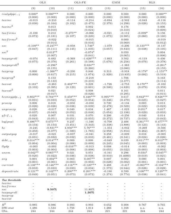
From a long-run perspective, and regarding tax items effects on households’ consumption, our results (presented in table 4) led us to conclude for a positive linear effect of raising rev-enues from taxes on goods and services, in percentage of GDP, while increasing revrev-enues from taxes on firms’ income and social security contributions seems to be detrimental for aggregate consumption Moreover, social contribution is the most harmful tax-item for households’ con-sumption. In in specific, an increase of 1% of this tax-item revenue, as percentage of GDP implies a reduction of 0.3%, approximately, of household’s final consumption.
Looking at the effects of the control variables on households’ consumption, we conclude for a negligible influence of both types of government expenditures. In addition, productive government spending, population growth, human capital, government debt, unemployment and deposit rates boost aggregate household consumption. Moreover, we conclude for consumption reduction when the current account balance improves and when there is an increase in money supply.
Regarding the non-linear tax effects analysis on households’ consumption, we only find tax items threshold values for taxes on payroll and social security contribution. While we find a minimizing value of 1.30% for payroll taxes, as a percentage of GDP, we find both maximizing and minimizing optimal values for social security contributions. Regarding this last tax item, although the results show a minimizing value of 9.50% we also achieve a maximum value of 11.80%. Therefore, we can conclude for an optimal interval of this tax to promote, or not, household consumption.
Table 4
The long-run analysis of taxation structure on income inequalities shows a similar pattern as the one observed in the short-run analysis for non-linear connections between tax structures and household income gaps (see table 5). For income taxation and taxes on consumption of goods and services, we find average maximizing values of 6.94% and 11.83%, respectively and on average, meaning that those tax items, in GDP proportion, enhance income disparities. On the other hand, we find mean minimizing values of 7.80% for firm’s taxation, 15.51% for social security contributions, and mean values of 1.00% and 1.53% for payroll and property taxes, respectively, which reduces the Gini index coefficient. In terms of the linear relationships, we do not conclude for a clear pattern for individual income taxes and payroll and workforce taxation. Furthermore, and as it is recognized by the literature, an increase in the GDP proportion of consumption taxes is associated with a higher degree of inequalities. Beyond the effect of this tax source, our results also show that higher old-age dependency ratios favour inequality growth. On the other hand, an increase in investment, through gross fixed capital formation and in human capital, a higher government spending related to social protection and education, among other factors support the political goals of reducing income inequalities.
Table 5
5
Concluding Remarks
In this paper, we have studied the tax structure impacts on both household aggregate consumption and income inequalities.
Through a panel set up, we analyse both short and long-term impacts of taxation structure and the effects on consumption, and find that while there are little non-linear relationships between taxes and consumption, all the considered tax items impact on household income disparities. In particular, and regarding households’ consumption, we only find a minimizing threshold value for payroll taxes, in a short and long run perspective, while we find a thresholds interval for social security contribution only for long-term. In addition, we uncover both mini-mizing and maximini-mizing optimum values of each tax item that affects household consumption.
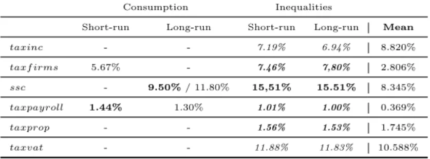
In terms of the tax items effects on the Gini index dynamics, we find minimizing effects on income disparities for firms’ taxation, social security contributions and payroll and property taxes, while consumption and personal income taxes seem to increase income gaps. The possible surprising effect of income taxation as a negative factor for income disparities may have to do with the fact of an inefficient progressive tax system, taxing several individual income sources in different ways that increase income inequalities. Table 6 summarizes the several tax items thresholds that we found in our analysis.
Table 6
References
Alm, J. and El-Ganainy, A. (2013). Value-added taxation and consumption. International Tax and Public Finance, 20(1):105–128.
Blanchard, O. and Perotti, R. (2002). An Empirical Characterization of the Dynamic Ef-fects of Changes in Government Spending and Taxes on Output. The Quarterly Journal of Economics, 117(4):1329–1368.
Carmignani, F. (2008). The impact of fiscal policy on private consumption and social outcomes in Europe and the CIS. Journal of Macroeconomics, 30(1):575 – 598.
Cingano, F. (2014). Trends in income inequality and its impact on economic growth. OECD Social, Employment and Migration Working Papers 163.
Clark, J. R. and Lawson, R. A. (2008). The Impact of Economic Growth, Tax Policy and Economic Freedom on Income Inequality. The Journal of Private Enterprise, 24(1):23–31. Duncan, D. and Sabirianova Peter, K. (2016). Unequal inequalities: Do progressive taxes reduce
income inequality? International Tax and Public Finance, 23(4):762–783.
Feenstra, R. C., Inklaar, R., and Timmer, M. P. (2015). The Next Generation of the Penn World Table. American Economic Review, 105(10):3150–3182.
Iosifidi, M. and Mylonidis, N. (2017). Relative effective taxation and income inequality: Evi-dence from OECD countries. Journal of European Social Policy, 27(1):57–76.
Islam, M. R., Madsen, J. B., and Doucouliagos, H. (2017). Does inequality constrain the power to tax? Evidence from the OECD. European Journal of Political Economy.
Mo, P. H. (2000). Income Inequality and Economic Growth. Kyklos, 53(3):293–315.
Mountford, A. and Uhlig, H. (2009). What are the effects of fiscal policy shocks? Journal of Applied Econometrics, 24(6):960–992.
Ostry, J. D., Berg, A., and Tsangarides, C. G. (2014). Redistribution, Inequality, and Growth. Staff Discussion Notes 14/02, International Monetary Fund.
Piketty, T. (2014). Capital in the twenty-first century. The Belknap Press of Harvard University Press, London, United Kingdom.
Piketty, T. and Saez, E. (2003). Income Inequality in the United States, 1913-1998. The Quarterly Journal of Economics, 118(1):1–39.
Romer, C. D. and Romer, D. H. (2010). The Macroeconomic Effects of Tax Changes: Estimates Based on a New Measure of Fiscal Shocks. The American Economic Review, 100(3):763–801. Saez, E. (2004). Direct or indirect tax instruments for redistribution: short-run versus long-run.
Journal of Public Economics, 88(3):503 – 518.
Solt, F. (2016). The Standardized World Income Inequality Database. Social Science Quarterly, 97. SWIID Version 6.1, October 2017.
Yi, D. J. (2012). No taxation, no democracy? taxation, income inequality, and democracy. Journal of Economic Policy Reform, 15(2):71–92.
6
Appendix
Table 1: Summary statistics of the variables set for income, consumption and inequalities, 1980-2015.
realgdppc taxinc taxfirms ssc taxpayroll taxprop taxvat
Mean 24.448 8.820 2.806 8.345 0.369 1.745 10.588
Std dev 14.313 4.635 1.500 4.981 0.728 1.003 3.046
Max 101.054 26.780 12.594 19.173 5.661 7.334 18.730
Min 2.184 0.873 0.261 0.000 0.000 0.074 2.979
Obs. 1195 1106 1106 1137 1137 1137 1137
hconsggdp proexp unproexp gfcf pop hc outputgap
Mean 56.382 27.536 16.71 23.161 33.531 3.02 -0.319
Std dev 7.069 4.24 4.837 4.091 52.235 0.435 2.850
Max 79.551 48.082 28.285 39.404 319.449 3.734 14.911
Min 29.918 0.537 0.000 11.546 0.228 1.469 -11.437
Obs. 1174 586 586 1174 1173 1173 851
debt llgdp unem avg current depositrate rtfpna
Mean 55.728 72.91 7.349 1797.237 -0.578 9.253 0.941
Std dev 35.901 48.689 3.835 249.343 5.565 25.364 0.123
Max 242.113 399.114 27.467 2911 16.467 682.53 1.539
Min 3.664 6.865 1.854 1361.7 -23.201 -0.18 0.472
Obs. 943 1139 741 986 727 1055 1173
pubser def pubor eco env hou hea
Mean 6.703 1.681 1.698 4.760 0.689 0.756 5.901
Std dev 2.274 1.333 0.440 1.763 0.346 0.440 1.686
Max 16.701 8.851 3.761 25.280 1.758 5.411 9.123
Min 2.980 0.000 0.815 1.307 -0.284 -0.083 0.379
Obs. 585 586 585 585 583 585 585
cul edu socpro ageratioold foreigninvestment gini
Mean 1.176 5.394 15.562 20.094 3.645 30.440
Std dev 0.570 1.080 4.708 5.519 10.487 6.562
Max 3.630 8.116 26.180 42.653 252.308 51.170
Min 0.248 3.021 5.440 6.641 -58.323 18.180
Table 2: Linear and non-linear short-run impact results of taxation structure on household consumption. OLS OLS-FE 2SLS RLS (1) (2) (3) (4) (5) (6) (7) (8) realgdppc−1 0.000 0.000** 0.000 0.000 0.000 0.000 0.000 0.000* (0.000) (0.000) (0.000) (0.000) (0.000) (0.000) (0.000) (0.000) taxinc 0.004 -0.108 -0.013 -0.130 -0.258 -0.610 0.022 0.046 (0.033) (0.176) (0.130) (0.433) (0.898) (1.511) (0.025) (0.147) taxinc2 0.006 0.002 0.046 -0.001 (0.010) (0.021) (0.105) (0.008) taxf irms -0.016 0.297 -0.393*** -0.204 -0.053 0.010 -0.040 0.261* (0.070) (0.215) (0.139) (0.223) (0.425) (0.674) (0.058) (0.152) taxf irms2 -0.025 -0.015 -0.008 -0.023** (0.016) (0.018) (0.050) (0.012) ssc -0.044 -0.060 0.038 1.785 -0.439 -0.107 -0.055 0.014 (0.053) (0.135) (0.136) (1.110) (1.146) (0.390) (0.036) (0.100) ssc2 0.005 -0.072 0.017 -0.001 (0.008) (0.044) (0.027) (0.006) taxpayroll -0.158* 0.072 -0.636* -2.093** -0.787 0.983 -0.044 -0.023 (0.088) (0.406) (0.352) (0.903) (2.175) (1.950) (0.073) (0.360) taxpayroll2 -0.106 0.728* -0.492 -0.021 (0.162) (0.389) (0.666) (0.147) taxprop -0.277*** -0.251 0.151 1.491 -0.032 -3.740 -0.227*** -0.630 (0.088) (0.492) (0.198) (1.043) (0.763) (4.802) (0.088) (0.494) taxprop2 -0.053 -0.289 0.628 0.076 (0.119) (0.200) (0.854) (0.109) taxvat 0.086 -0.172 0.324** 1.012 -0.748 -1.535 0.091 -0.489 (0.102) (0.455) (0.151) (0.714) (2.508) (1.683) (0.076) (0.341) taxvat2 0.013 -0.028 0.072 0.026* (0.019) (0.029) (0.098) (0.014) hconsggdp−1 0.861*** 0.861*** 0.552*** 0.550*** 0.948*** 0.802*** 0.873*** 0.865*** (0.036) (0.035) (0.061) (0.062) (0.143) (0.171) (0.024) (0.026) proexp 0.023 0.031 -0.051 -0.046 0.258 -0.046 0.008 0.018 (0.029) (0.030) (0.048) (0.047) (0.927) (0.129) (0.021) (0.022) unproexp 0.051 0.029 0.079 0.074 0.642 -0.210 0.034 0.007 (0.044) (0.044) (0.054) (0.051) (1.928) (0.696) (0.027) (0.031) gf cf−1 0.011 0.010 -0.012 0.040 0.093 -0.122 -0.012 -0.050 (0.055) (0.070) (0.076) (0.077) (0.142) (0.261) (0.032) (0.040) log(pop) 0.342** 0.408*** -4.642 -5.121 -0.267 0.726 0.340*** 0.392*** (0.142) (0.142) (5.091) (5.059) (1.339) (1.363) (0.117) (0.136) hc 0.119 0.069 1.835 2.645 -0.883 -2.117 -0.127 -0.193 (0.272) (0.388) (1.984) (1.680) (1.249) (2.038) (0.250) (0.349) outputgap -0.098*** -0.108*** -0.065 -0.069 0.049 -0.041 -0.079*** -0.098*** (0.036) (0.038) (0.049) (0.051) (0.174) (0.137) (0.023) (0.024) debt−1 0.008** 0.007* 0.008 0.002 -0.012 0.018 0.008*** 0.005 (0.003) (0.004) (0.010) (0.010) (0.094) (0.017) (0.003) (0.003) llgdp -0.002 -0.004 -0.027*** -0.022*** -0.003 -0.013 0.000 -0.003 (0.003) (0.004) (0.008) (0.008) (0.021) (0.009) (0.003) (0.003) unem 0.007 0.018 0.040 0.076 -0.074 0.077 0.008 0.011 (0.018) (0.020) (0.048) (0.048) (0.355) (0.150) (0.018) (0.020) avg 0.001 0.001 0.004 0.008** 0.003 0.002 0.000 0.000 (0.001) (0.001) (0.003) (0.003) (0.011) (0.001) (0.001) (0.001) current -0.160*** -0.168*** -0.179*** -0.172*** 0.132 -0.213 -0.139*** -0.16*** (0.038) (0.041) (0.047) (0.050) (0.598) (0.302) (0.025) (0.027) depositrate 0.044 0.049 0.073 0.074 0.066 0.361 0.066* 0.100** (0.046) (0.053) (0.080) (0.082) (0.485) (0.260) (0.037) (0.039) Tax tresholds taxinc - - - -taxf irms - - - 5.67% ssc - - - -taxpayroll - - - 1.44% - - - -taxprop - - - -taxvat - - - -R2 0.984 0.984 0.991 0.992 0.937 0.974 0.768 0.782
DW-stat 1.941 1.963 2.145 2.133 1.489 1.755 n.a. n.a.
Obs. 244 244 244 244 221 221 244 244
Notes: *, ** and *** represent statistical significance at levels of 10%, 5% and 1% respectively. The robust standard errors are in brackets. The White diagonal covariance matrix is used in order to assume residual heterokedasticity, with the exception for RLS technique. The DW-statistic is the Durbin-Watson statistic. The non-bold and bold values express, respectively, maximum and minimum optimal tax items levels.
Table 3: Linear and non-linear short-run impact results of taxation structure on household income inequalities. OLS OLS-FE GMM RLS (1) (2) (3) (4) (5) (6) (7) (8) realgdppc−1 0.000*** 0.000*** 0 0.000*** 0.000*** 0.000*** 0.000*** 0.000*** (0.000) (0.000) (0.000) (0.000) (0.000) (0.000) (0.000) (0.000) taxinc -0.099** 0.281*** -0.003 0.328** -0.080 0.352*** -0.149*** 0.196*** (0.049) (0.092) (0.080) (0.155) (0.052) (0.1000) (0.038) (0.063) taxinc2 -0.019*** -0.023*** -0.020*** -0.018*** (0.003) (0.008) (0.004) (0.002) taxf irms -0.398*** -1.305*** -0.075 -0.243** -0.399*** -1.759*** -0.177*** -0.950*** (0.076) (0.185) (0.082) (0.115) (0.080) (0.252) (0.054) (0.117) taxf irms2 0.082*** 0.01 0.128*** 0.063*** (0.015) (0.007) (0.023) (0.01) ssc -0.297*** -0.529*** -0.295** -1.179*** -0.304*** -0.615*** -0.319*** -0.622*** (0.04) (0.114) (0.122) (0.324) (0.042) (0.141) (0.035) (0.082) ssc2 -0.002 0.038*** 0.004 0.002 (0.008) (0.013) (0.01) (0.005) taxpayroll 0.668*** -2.029*** -0.359 -1.645*** 0.621*** -1.681*** 0.567*** -1.761*** (0.162) (0.573) (0.407) (0.43) (0.163) (0.599) (0.112) (0.365) taxpayroll2 1.023*** 0.795*** 0.84*** 0.872*** (0.239) (0.199) (0.251) (0.152) taxprop -0.135 -2.904*** -0.083 -0.587 -0.326* -3.407*** 0.337*** -0.928** (0.167) (0.605) (0.243) (0.601) (0.187) (0.613) (0.124) (0.382) taxprop2 0.845*** 0.086 0.95*** 0.392*** (0.131) (0.119) (0.145) (0.088) taxvat 0.005 0.862*** -0.127 0.771*** -0.085 0.518 0.014 1.660*** (0.094) (0.320) (0.100) (0.275) (0.102) (0.380) (0.063) (0.218) taxvat2 -0.033** -0.036*** -0.024 -0.070*** (0.016) (0.012) (0.017) (0.010) avg 0.004*** 0.004*** -0.001 -0.001 0.004*** 0.004*** 0.006*** 0.007*** (0.001) (0.001) (0.002) (0.001) (0.001) (0.001) (0.001) (0.001) unem 0.171*** 0.151*** 0.113*** 0.111*** 0.154*** 0.125*** 0.138*** 0.125*** (0.035) (0.030) (0.031) (0.018) (0.035) (0.029) (0.027) (0.019) log(pop) 0.676*** 0.856*** 4.122 5.447*** 0.664*** 0.723*** 0.479*** 0.859*** (0.164) (0.162) (3.758) (1.825) (0.165) (0.146) (0.116) (0.094) hc -5.123*** -4.277*** -0.862 -0.047 -5.372*** -4.933*** -3.696*** -2.695*** (0.402) (0.556) (1.407) (0.872) (0.398) (0.576) (0.308) (0.336) rtf pna 4.161** 5.833*** 0.046 0.071 3.797* 5.994*** -0.690 -1.166 (2.029) (2.075) (2.133) (1.097) (1.961) (1.775) (1.44) (1.155) pubser -0.537*** -0.416*** 0.175*** 0.202*** -0.532*** -0.444*** -0.341*** -0.229*** (0.084) (0.080) (0.060) (0.061) (0.083) (0.078) (0.063) (0.049) def 1.241*** 1.080*** -0.153 -0.016 1.323*** 1.169*** 1.034*** 0.868*** (0.123) (0.146) (0.180) (0.145) (0.128) (0.133) (0.087) (0.078) pubor 2.050*** 1.614*** -0.205 -0.298 2.190*** 1.706*** 2.597*** 0.980*** (0.433) (0.418) (0.247) (0.237) (0.410) (0.351) (0.281) (0.231) eco -0.208** -0.260*** -0.047* -0.045 -0.183* -0.230*** -0.233*** -0.277*** (0.099) (0.088) (0.027) (0.032) (0.094) (0.057) (0.053) (0.039) env -2.293*** -0.957** -0.141 -0.230 -2.159*** -0.881** -2.959*** -0.723*** (0.466) (0.416) (0.330) (0.270) (0.457) (0.341) (0.303) (0.230) hou 0.600 0.907** 0.391 0.250 0.620 0.850*** 0.750*** 1.071*** (0.438) (0.434) (0.295) (0.153) (0.433) (0.280) (0.236) (0.187) hea -0.164 -0.276** 0.181 0.107 -0.158 -0.298*** -0.084 -0.355*** (0.119) (0.134) (0.146) (0.099) (0.121) (0.097) (0.071) (0.061) cul 1.122** 0.541 0.594 0.971*** 1.270*** 0.560* 2.276*** 1.849*** (0.486) (0.511) (0.454) (0.283) (0.485) (0.326) (0.254) (0.201) edu -0.663*** -0.445** 0.209 0.207 -0.689*** -0.573*** -0.781*** -0.335*** (0.178) (0.188) (0.215) (0.140) (0.170) (0.164) (0.133) (0.108) socpro -0.284*** -0.198*** -0.271*** -0.287*** -0.265*** -0.165*** -0.290*** -0.157*** (0.048) (0.060) (0.066) (0.045) (0.049) (0.043) (0.035) (0.029) ageratioold 0.294*** 0.291*** 0.121** 0.106*** 0.287*** 0.273*** 0.346*** 0.377*** (0.031) (0.031) (0.053) (0.035) (0.032) (0.028) (0.023) (0.018) depositrate 0.155*** 0.15*** -0.039 -0.052** 0.157*** 0.129*** -0.081*** -0.018 (0.045) (0.035) (0.036) (0.024) (0.045) (0.034) (0.031) (0.023) f oreigninvestment -0.011* -0.007 0.001 0.000 -0.012* -0.007 -0.004 -0.003 (0.006) (0.005) (0.004) (0.003) (0.006) (0.007) (0.007) (0.005) gf cf -0.106** -0.061* -0.001 -0.008 -0.126*** -0.081** -0.127*** -0.030 (0.041) (0.035) (0.050) (0.030) (0.041) (0.033) (0.030) (0.022) hconsggdp -0.036** -0.053*** -0.014 -0.018 -0.031* -0.069*** -0.028** -0.029*** (0.016) (0.014) (0.018) (0.016) (0.016) (0.016) (0.013) (0.010) Tax thresholds taxinc - 7.39% - 7.13% - 8.80% - 5.44% taxf irms - 7.96% - - - 6.87% - 7.54% ssc - - - 15.51% - - - -taxpayroll - 0.99% - 1.03% - 1.00% - 1.01% taxprop - 1.72% - - - 1.79% - 1.18% taxvat - 13.06% - 10.71% - - - 11.86% R2 0.893 0.932 0.990 0.992 0.894 0.930 0.739 0.773
DW-stat 0.351 0.531 0.622 0.763 0.335 0.594 n.a. n.a.
Obs. 361 361 361 361 360 360 361 361
Notes: *, ** and *** represent statistical significance at levels of 10%, 5% and 1% respectively. The robust standard errors are in brackets. The White diagonal covariance matrix is used in order to assume residual heterokedasticity, with the exception for RLS technique. The DW-statistic is the Durbin-Watson statistic. The non-bold and bold values express, respectively, maximum and minimum optimal tax items levels.
Table 4: Linear and non-linear long-run impact results of taxation structure on household consumption. OLS OLS-FE GMM RLS (9) (10) (11) (12) (13) (14) (15) (16) realgdppc−1 0.000* 0.000*** 0.000 0.000 0.000 0.000 0.000 0.000** (0.000) (0.000) (0.000) (0.000) (0.000) (0.000) (0.000) (0.000) taxinc -0.013 -0.210 -0.114 -0.214 -0.694 -2.502 -0.043 -0.116 (0.030) (0.164) (0.102) (0.475) (2.379) (4.298) (0.026) (0.155) taxinc2 0.013 0.002 0.176 0.006 (0.010) (0.024) (0.310) (0.009) taxf irms -0.100 0.212 -0.275** -0.066 -0.021 -0.112 -0.099* 0.156 (0.072) (0.181) (0.107) (0.220) (1.073) (0.985) (0.060) (0.160) taxf irms2 -0.022 -0.015 0.000 -0.019 (0.014) (0.016) (0.069) (0.012) ssc -0.109** -0.247** -0.058 1.746* -1.079 -0.206 -0.133*** -0.137 (0.047) (0.111) (0.145) (1.035) (3.057) (0.843) (0.038) (0.105) ssc2 0.013** -0.074* 0.050 0.004 (0.007) (0.041) (0.065) (0.006) taxpayroll -0.074 0.492 -0.369 -1.626*** -1.663 3.502 -0.119 0.436 (0.075) (0.378) (0.261) (0.588) (5.676) (6.256) (0.076) (0.378) taxpayroll2 -0.296* 0.624** -1.383 -0.261* (0.155) (0.260) (2.080) (0.155) taxprop 0.000 -1.366** -0.230 0.846 0.313 -9.918 -0.179* -1.155** (0.000) (0.617) (0.215) (1.074) (1.929) (13.835) (0.092) (0.519) taxprop2 0.153 -0.218 1.706 0.163 (0.133) (0.210) (2.377) (0.114) taxvat 0.181* -0.263 0.402*** 0.228 -1.726 -2.753 0.170** -0.102 (0.102) (0.395) (0.129) (0.601) (6.500) (4.820) (0.079) (0.359) taxvat2 0.021 0.008 0.161 0.011 (0.017) (0.026) (0.295) (0.015) hconsggdp−1 0.802*** 0.784*** 0.458*** 0.448*** 0.995*** 0.617 0.842*** 0.826*** (0.031) (0.033) (0.052) (0.054) (0.346) (0.479) (0.025) (0.027) proexp 0.006 0.018 -0.050 -0.050 0.720 -0.134 0.003 0.013 (0.026) (0.026) (0.038) (0.039) (2.478) (0.509) (0.022) (0.023) unproexp 0.026 -0.017 0.040 0.034 1.467 -1.023 0.051* 0.017 (0.037) (0.043) (0.052) (0.048) (5.054) (2.198) (0.029) (0.033) gf cf−1 0.020 0.007 0.031 0.070 0.206 -0.256 0.040 0.014 (0.043) (0.051) (0.051) (0.055) (0.372) (0.737) (0.034) (0.042) log(pop) 0.486*** 0.675*** 0.237 -1.346 -0.708 2.406 0.361*** 0.477*** (0.134) (0.154) (3.451) (3.343) (3.338) (3.888) (0.123) (0.143) hc -0.245 -0.831** 4.956*** 5.76*** -1.354 -4.842 -0.269 -0.566 (0.258) (0.377) (1.580) (1.785) (2.958) (5.854) (0.262) (0.367) outputgap -0.017 -0.021 -0.037 -0.041 0.258 -0.009 0.016 -0.003 (0.031) (0.032) (0.032) (0.033) (0.481) (0.341) (0.024) (0.026) debt−1 0.014*** 0.014*** 0.009 0.006 -0.049 0.039 0.011*** 0.012*** (0.004) (0.004) (0.008) (0.009) (0.245) (0.045) (0.003) (0.003) llgdp -0.003 -0.003 -0.016** -0.013 0.008 -0.014 -0.001 -0.002 (0.003) (0.004) (0.008) (0.008) (0.055) (0.022) (0.003) (0.003) unem 0.042** 0.065*** 0.021 0.051 -0.161 0.296 0.034* 0.045** (0.020) (0.022) (0.036) (0.038) (0.910) (0.4000) (0.019) (0.021) avg 0.001 0.002** 0.003 0.007** 0.007 0.002 0.000 0.001 (0.001) (0.001) (0.003) (0.003) (0.028) (0.002) (0.001) (0.001) current -0.138*** -0.146*** -0.116*** -0.120*** 0.488 -0.417 -0.083*** -0.104*** (0.033) (0.033) (0.033) (0.034) (1.573) (0.944) (0.026) (0.028) depositrate 0.121** 0.142*** 0.200*** 0.201*** -0.190 0.599 0.100*** 0.129*** (0.049) (0.051) (0.073) (0.072) (1.274) (0.774) (0.038) (0.041) Tax thresholds taxinc - - - -taxf irms - - - -ssc - 9.50% - 11.80% - - - -taxpayroll - - - 1.30% - - - -taxprop - - - -taxvat - - - -R2 0.985 0.986 0.993 0.993 0.652 0.908 0.767 0.765
DW-stat 1.486 1.534 1.756 1.814 1.266 1.168 n.a. n.a.
Obs. 244 244 244 244 221 221 244 244
Notes: *, ** and *** represent statistical significance at levels of 10%, 5% and 1% respectively. The robust standard errors are in brackets. The White diagonal covariance matrix is used in order to assume residual heterokedasticity, with the exception for RLS technique. The DW-statistic is the Durbin-Watson statistic. The non-bold and bold values express, respectively, maximum and minimum optimal tax items levels.
Table 5: Linear and non-linear long-run impact results of taxation structure on household income inequalities. OLS OLS-FE GMM RLS (9) (10) (11) (12) (13) (14) (15) (16) realgdppc−1 0.000*** 0.000*** 0.000*** 0.000*** 0.000*** 0.000** 0.000*** 0.000*** (0.000) (0.000) (0.000) (0.000) (0.000) (0.000) (0.000) (0.000) taxinc -0.086* 0.253*** 0.043 0.328** -0.079 0.311*** -0.140*** 0.146** (0.047) (0.092) (0.047) (0.155) (0.052) (0.105) (0.038) (0.062) taxinc2 -0.017*** -0.023*** -0.018*** -0.016*** (0.003) (0.008) (0.004) (0.002) taxf irms -0.388*** -1.190*** 0.024 -0.243** -0.410*** -1.706*** -0.197*** -0.863*** (0.070) (0.180) (0.050) (0.115) (0.081) (0.286) (0.053) (0.117) taxf irms2 0.072*** 0.010 0.122*** 0.053*** (0.015) (0.007) (0.029) (0.010) ssc -0.290*** -0.487*** -0.281*** -1.179*** -0.303*** -0.594*** -0.315*** -0.578*** (0.039) (0.119) (0.062) (0.324) (0.042) (0.137) (0.034) (0.082) ssc2 -0.004 0.038*** 0.003 0.000 (0.008) (0.013) (0.010) (0.005) taxpayroll 0.700*** -1.854*** -0.149 -1.645*** 0.642*** -1.689** 0.591*** -1.552*** (0.164) (0.582) (0.198) (0.430) (0.167) (0.658) (0.110) (0.365) taxpayroll2 0.970*** 0.795*** 0.862*** 0.772*** (0.240) (0.199) (0.276) (0.152) taxprop -0.114 -2.930*** 0.091 -0.587 -0.305 -3.330*** 0.280** -0.802** (0.167) (0.646) (0.128) (0.601) (0.187) (0.71) (0.122) (0.381) taxprop2 0.849*** 0.086 0.938*** 0.368*** (0.137) (0.119) (0.150) (0.088) taxvat 0.017 0.894*** -0.056 0.771*** -0.069 0.514 -0.015 1.745*** (0.095) (0.322) (0.073) (0.275) (0.102) (0.375) (0.061) (0.217) taxvat2 -0.034** -0.036*** -0.023 -0.075*** (0.015) (0.012) (0.018) (0.010) avg 0.004*** 0.003*** 0.000 -0.001 0.004*** 0.004*** 0.006*** 0.007*** (0.001) (0.001) (0.001) (0.001) (0.001) (0.001) (0.001) (0.001) unem 0.154*** 0.135*** 0.106*** 0.111*** 0.143*** 0.115*** 0.124*** 0.094*** (0.034) (0.03) (0.017) (0.018) (0.035) (0.031) (0.026) (0.019) log(pop) 0.667*** 0.873*** 5.405*** 5.447*** 0.672*** 0.745*** 0.555*** 0.87*** (0.159) (0.163) (1.649) (1.825) (0.163) (0.172) (0.115) (0.094) hc -5.182*** -4.323*** 0.143 -0.047 -5.371*** -4.893*** -3.794*** -2.609*** (0.381) (0.555) (0.768) (0.872) (0.385) (0.689) (0.303) (0.335) rtf pna 4.989** 6.322*** 1.395 0.071 4.758** 6.858*** 0.426 -0.417 (2.027) (2.072) (0.996) (1.097) (2.007) (2.098) (1.420) (1.153) pubser -0.575*** -0.444*** 0.178*** 0.202*** -0.556*** -0.463*** -0.326*** -0.221*** (0.083) (0.082) (0.041) (0.061) (0.084) (0.086) (0.062) (0.049) def 1.313*** 1.134*** -0.051 -0.016 1.380*** 1.220*** 1.057*** 0.846*** (0.127) (0.150) (0.135) (0.145) (0.135) (0.175) (0.086) (0.078) pubor 2.307*** 1.885*** 0.030 -0.298 2.369*** 1.948*** 2.506*** 1.130*** (0.423) (0.416) (0.188) (0.237) (0.421) (0.423) (0.277) (0.230) eco -0.194** -0.245*** -0.054* -0.045 -0.177* -0.227*** -0.221*** -0.207*** (0.096) (0.085) (0.029) (0.032) (0.093) (0.080) (0.053) (0.039) env -2.432*** -1.159*** -0.541*** -0.230 -2.310*** -1.112*** -2.783*** -1.133*** (0.436) (0.400) (0.184) (0.270) (0.435) (0.390) (0.299) (0.229) hou 0.571 0.840* 0.307* 0.250 0.585 0.797* 0.706*** 0.905*** (0.439) (0.441) (0.170) (0.153) (0.436) (0.451) (0.233) (0.187) hea -0.176 -0.273* 0.249** 0.107 -0.162 -0.290** -0.118* -0.310*** (0.122) (0.140) (0.097) (0.099) (0.126) (0.146) (0.07) (0.061) cul 1.049** 0.523 0.900*** 0.971*** 1.169** 0.456 2.218*** 2.025*** (0.507) (0.533) (0.305) (0.283) (0.510) (0.533) (0.251) (0.201) edu -0.724*** -0.496*** 0.260** 0.207 -0.714*** -0.576*** -0.699*** -0.359*** (0.165) (0.181) (0.113) (0.14) (0.166) (0.187) (0.131) (0.108) socpro -0.276*** -0.199*** -0.306*** -0.287*** -0.258*** -0.170*** -0.277*** -0.155*** (0.046) (0.058) (0.038) (0.045) (0.047) (0.059) (0.035) (0.028) ageratioold 0.299*** 0.296*** 0.106*** 0.106*** 0.290*** 0.275*** 0.331*** 0.366*** (0.031) (0.032) (0.028) (0.035) (0.032) (0.033) (0.022) (0.018) depositrate 0.162*** 0.158*** -0.022 -0.052** 0.162*** 0.136*** -0.079*** -0.028 (0.050) (0.040) (0.029) (0.024) (0.049) (0.042) (0.03) (0.023) f oreigninvestment -0.009 -0.006 0.001 0.000 -0.009 -0.004 -0.003 -0.002 (0.006) (0.005) (0.002) (0.003) (0.006) (0.005) (0.007) (0.005) gf cf -0.114*** -0.074** -0.021 -0.008 -0.126*** -0.083** -0.119*** -0.046** (0.041) (0.036) (0.023) (0.030) (0.041) (0.037) (0.029) (0.022) hconsggdp -0.035*** -0.049*** -0.015 -0.018 -0.028* -0.064*** -0.022* -0.022** (0.016) (0.014) (0.016) (0.016) (0.016) (0.015) (0.013) (0.010) Tax thresholds taxinc - 7.44% - 7.13% - 8.64% - 4.56% taxf irms - 8.26% - - - 6.99% - 8.14% ssc - - - 15.51% - - - -taxpayroll - 0.96% - 1.03% - 0.98% - 1.01% taxprop - 1.73% - - - 1.78% - 1.09% taxvat - 13.15% - 10.71% - . - 11.63% R2 0.897 0.932 0.992 0.992 0.896 0.929 0.749 0.786
DW-stat 0.386 0.554 1.042 0.763 0.376 0.627 n.a. n.a.
Obs. 362 362 362 362 361 361 362 362
Notes: *, ** and *** represent statistical significance at levels of 10%, 5% and 1% respectively. The robust standard errors are in brackets. The White diagonal covariance matrix is used in order to assume residual heterokedasticity, with the exception for RLS technique. The DW-statistic is the Durbin-Watson statistic. The non-bold and bold values express, respectively, maximum and minimum optimal tax items levels.
Table 6: Summary of tax items threshold values for households’ consumption and inequalities.
Consumption Inequalities
Short-run Long-run Short-run Long-run Mean
taxinc - - 7.19% 6.94% 8.820% taxf irms 5.67% - 7.46% 7,80% 2.806% ssc - 9.50% / 11.80% 15,51% 15.51% 8.345% taxpayroll 1.44% 1.30% 1.01% 1.00% 0.369% taxprop - - 1.56% 1.53% 1.745% taxvat - - 11.88% 11.83% 10.588%
Notes: The non-bold and bold values presented in the short-run and long-run columns express, respectively, the maximum and minimum optimal tax items levels. The values expressed in italics represent average values.