doi: 10.1590/0101-7438.2018.038.02.0173
A GENERALIZED DECOMPOSITION ALGORITHM FOR REAL-TIME TRUCK ROUTING PROBLEMS
Yihua Li
1, Qing Miao
2*and Xiubin Bruce Wang
3Received April 29, 2017 / Accepted March 17, 2018
ABSTRACT.This paper is based on a practical project jointly conducted by a major trucking company and a renowned operations research consulting firm. It studies a large-scale, real-time truckload pickup and delivery problem. A number of cost factors are carefully measured such as loaded/empty travel distance, travel time, crew labor, equipment rental or operational cost, and revenue for completing the movements. This paper proposes a generalized decomposition algorithm that is capable of considering sophisticated business rules. The goal is to recommend executable and efficient truck routing decisions to minimize operating costs. Numerical tests are conducted with operational data from J.B.HUNT. A fleet of 5,000 trucks is considered in this experiment. The test result not only shows significant cost savings but also demonstrates computational efficiency for real-time application.
Keywords: Truck routing, decomposition algorithm, column generation.
1 INTRODUCTION
Research on vehicle routing has seen wide applications in the transportation industry such as truck, railway, airline and pipeline, which saves on costs while covers more demands. The ob-jective is to improve the fleet operational efficiency. This research is important within the con-text of increasingly automated (or computerized) systems to support decision making for the routing/scheduling routines. It can be easily extended to solving other problems that may look seemingly different, but belong to the same family of NP-completeness (Li et al., 2010, 2012 and 2014). The social economic impact of this problem cannot be overestimated. In the past century, especially during the last 60 years, numerous research efforts have been made specially to solve the trucking industry’s routing problems.
*Corresponding author.
1United Airlines, Willis Tower, 233 South. Wacker Drive, Chicago, IL 60606, United States. E-mail: yihua.li@united.com
2The Home Depot, 2455 Paces Ferry Rd SE, Atlanta, GA 30339-1834, United States. E-mail: qing miao@homedepot.com
The main contribution of this paper is to introduce a decomposition algorithm based on a practical project. The goal is to recommend executable and efficient truck routing decisions to minimize operating costs. Numerical tests are conducted with operational data from J.B.HUNT. The test result not only shows significant cost savings but also demonstrates computational efficiency for real-time application.
Within the company, a fleet of vehicles are to be scheduled and routed to serve a known set of loads, and each load is considered as a full truckload with an origin and a destination (OD) asso-ciated with time window constraints for pickup and delivery. There are a finite number of drivers (or, crew in general) available to be assigned. Each driver has to return home within a period of 14 days according to the company rule as well as union regulation to retain drivers (for example, maximum consecutive hours of driving). A route consists of a sequence of moves to be fulfilled by a single vehicle. A typical route needs to have a starting location the same as termination location, which makes a tour to the associated vehicle. Depending on the service type, certain vehicles or drivers may not be eligible. For example, Dedicated Contract Serviceis a service primarily utilizes semi-trailer trucks to transport cargo across the country; Intermodal Service
partners with railways, commercial airlines or port authorities to move containers. Furthermore, once the drivers are committed to certain loads, diversion is typically not allowed with the ex-ception from management approval. For the convenient purpose, this study does not consider diversion in the problem formulation and presentation.
The primary objective is to minimize the operation cost. In addition to cost of labor, other ma-jor costs include fuel rate, travel distance, equipment rental and length of operation. Revenue from serving each load can be considered as a positive profit or negative cost whenever a load is covered or service is completed. Empty truck moves and empty driver moves (also called
deadhead moves) do not generate revenue, thus are only considered costs to the company. It is expected that the developed algorithm is built into a decision making system to recommend routings automatically.
2 LITERATURE REVIEW
In contrast to the less-than-truckload where each vehicle carries multiple customer demands, truckload only allows a truck to serve a single customer demand each time. An example route of a vehicle starts from depot (or source), loads goods at a factory or warehouse, moves to the load destination facility, unloads the load before goes to another loading location and repeats the same truckload movement. In the end, the vehicle returns to the depot (Labadie & Prins, 2012). This is a typical vehicle routing/scheduling problem in literature.
with stochastic features drew more and more attention from the research community. These fea-tures included but were not limited to stochastic load distributions (Golden & Stewart, 1978; Stewart & Golden, 1983; and Bastian & Rinnooy Kan, 1992), stochastic travel time (Cook & Russell, 1978; and Berman & Simchi-Levi, 1989), or stochastic locations (Laporte et al., 1994; and Bertsimas & Howell, 1993). As the information technologies came into play, recent real-time and dynamic VRP problems became increasingly important (Yang et al., 2004). Powell et al. (1995) presented a survey of dynamic fleet optimizations dealing with some general issues. Later work of Powell et al. (2000) developed a practical model to consider dynamic assignment of drivers to known demands, which provided significant insights to our study problem here. Re-optimization policies are further introduced and tested in Yang, et al. (1998). The most recent reviews summarizing the state-of-art techniques are available in Laporte et al. (2013), Derigs et al. (2013), and Braekers et al. (2016).
Published articles on implementation, however, are less popular compared with the counterpart on theoretical studies. When it comes to practical VRP projects, people often look for details about how algorithms are developed and implemented. This paper is originated from industry projects within a major trucking company and focuses on proven practical techniques. Imple-mentation details are revealed so that the readers can have a better understanding of the business logic. It aims at utilizing a combined optimization method and advanced information technology to develop a real-time dispatching system. The computational time invested in searching for bet-ter decisions in bet-terms of shorbet-ter routes and more revenue should be cautiously balanced with the needs of coming up with a decision in a timely manner.
3 SOLUTION APPROACH
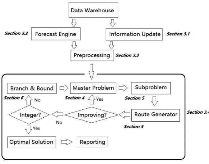
This decision support system requires a list of components to function properly. Information is updated via continuous data feed, stored in a centralized data warehouse. Forecast mod-ule provides projections on the existing truck moves and the estimation on the future demand. Prepossessing module turns the raw data into the format that are favored by the optimizer. Opti-mization component is the core module that handles the mathematical formulation and sophisti-cated algorithm.
3.1 Information Updating
3.2 Forecast Engine
Certain loads are visible before they become available for pickup. For example, the containers can be moved by trains with a projected arrival time at the pickup location. The forecast engine would gather the information from partnered carriers to make reasonable projections on the availability of their own loads. This helps the optimization engine to look beyond the current demands and make informed decision for the immediate future. Beyond the visible horizon, long term forecast is also necessary to plan ahead in terms of fleet sizing and infrastructure change at strategic level.
3.3 Preprocessing
The preprocessor needs to selectively package the raw data into the network format that the downstream optimizer requires. The basic elements in this network are link (edge) and node (vertex), which are explained in section 5. Examining the feasibility of the links can reduce the burden on the optimizer. For example, it needs to filter out an infeasible link that tries to merry a wrong type of truck to a load. Each node represents an activity such as getting a truck, load or unload. After excluding infeasible links, certain business rules will further reduce the number of links by checking the distance, time or any other resource consumed between two nodes. If certain link violates resource limit, then this link is also excluded. The ultimate goal here is to allow the optimization module find reliable routes through the network easily.
3.4 Optimization Strategy
Due to the complicated resource constraints and business rules, it is inconvenient to formulate this truck routing problem into a network flow model. The alternative approach is to apply parti-tion or set-covering model, where the objective funcparti-tion minimizes the combined cost of routes being selected.
Figure 1– Dependency Diagram and Flow Chart.
4 MASTER PROBLEM FORMULATION
Minimize
j∈k
cjxj (1)
subject to:
j∈k
δijxj =1 ∀i ∈ N, dualπi (2)
xj =0,1 ∀j ∈k (3)
where:
xj decision variable, 1 if route jis selected, 0 otherwise
k the set of routes in thek-th iteration of the column generation procedure
cj the cost associated with routej (operating cost – load revenue)
N the set of loads
δij if route jcovers loadi, 0 otherwise
πi dual associatedi-th constraint (for loadi)
It is important to note that during the iteration, the master problem is solved as linear program-ming relaxation to get dual values. The side constraints are conditional and are not formulated into the master. For example:
j∈k
xj ≤ D R
Although the company prefers its own salaried drivers over the contracted drivers due to the lowered operating cost. DRis the total number of both. When the total number of routes being selected exceeds limitDR, it is intuitive to sort the route costs in an ascending order to pick the firstDR. The uncovered loads can be either rejected or outsourced. This is to facilitate the construction of the subproblem, where all the dual values associated with Eq. (2) are utilized to reflect what master problem desires.
5 CONSTRAINED SHORTEST PATH SUBPROBLEM
Our subproblem tries to find an optimal path go through networkGthat does not consume more than limited resources, such as time window, duration of path, distance, etc. Because of the additional constraints applied to the path, the subproblem is therefore aConstrainedShortest Path Problem (CSPP). A path here represents a truck route in reality.
5.1 Subproblem Formulation
Minimize
(i,j)∈A
(ci j−πj)xi j
where
xi j are the decision variables, 1 if nodeiis followed by node j,0 otherwise
ci j the cost to proceed from nodeito nodej
A the set of eligible connections, link(i,j)∈ A
πj dual associated j-th constraint (for load j)
The construction of the subproblem is essential to the usefulness of the generated routes and the overall solution time. A route is a collection of links that are connected by nodes, it is also referred as a path through network. Since it has a single objective function to generate the most profitable route, different cost elements need to be normalized within the network. For example, the overall cost on linki to j is based on the load/empty factor, distance(i,j), the revenue of moving load j, and dualπj for load j. Given the same distance, an empty-truck move has a baseline cost and zero revenue. A loaded-truck move may double the baseline cost but gain revenue. The changing value ofπj is passed from master problem to adapt to the current need.
Each route begins from the source S and ends at sink T. In most cases, the source and sink are the same physical location but have different time windows. This is due to the business rule that the driver has to return to home terminal when the route is completed. Starting from source
Other resource constraints include (1) the maximum duration of each route, which is limited to 14 days; (2) the maximum combined travel distance for each route; (3) the time window for the load, which represents the earliest and latest time to pick up or deliver. In order to solve this multiple resource constrained shortest path problem with time windows, a specialized Label Setting Algorithm is applied.
5.2 The Algorithm for Shortest Path with Resource Constraints
Let(D∗ik,Cik)and(D∗j k,Cj k)be the labels representing two different paths to nodek. Then the first labeldominatesthe latter, if and only if(Dik∗,Cik)−(D∗j k,Cj k)≥(0,0). The first label is smaller thanthe latter, i.e.,(D∗
ik,Cik) L
<(D∗j k,Cj k), if and only if(D∗ik,Cik)=(D∗j k,Cj k), and the first non-null element of((Dik∗,Cik)−(D∗j k,Cj k))is positive. A label(Dk∗,Ck)is efficient if none of the labels at node k can dominate it. The path corresponding to an efficient label is defined as an efficient path. Only efficient labels and paths are kept.
LetQkbe the set of labels associated with the cost lower bound of path ending at nodek ∈ V, and Pk be the set of labels associated with feasible paths. The Pk defines the primal function. The primal function provides an upper bound on the cost of efficient solutions at nodek. When primal and dual functions have same value for a given stage, the labels inPandQare associated to an efficient path for the current stage.
Then the algorithm used to solve the subproblem is presented as follows:
Step 1. (Initialization).
PS = (0,0, . . . ,0),QS = (0,0, . . . ,0),Pi = ∅ (empty), Qi = (a1i,ai2, . . . ,aiL,−∞),
i∈V −S
Find(d∗j,cj)=minlex (i,j)∈A
(di j∗,ci j), for each node j∈V −S. O= j∈V−S
(Qj).
Step 2. (Calculation of the lexicographically smallest label inO).
IfO=∅, stop; [The current label(s) at the sink nodeT is (are) the shortest path(s)]. Otherwise, find the lexicographically smallest labelF(O)= minlex
(D∗j,Cj)∈O
(D∗j,Cj)=(D∗
′
j ,Cj).
Step 3. (Look for a label(D∗k′,Ck)∈ B(O)to be treated).
B(O)=
Dk∗,Ck∈O|F(O)
L ≤
D∗k,Ck
L
<F(O)+
dk∗,Ck.
Step 4. (Uncertainty zone).
Define the uncertainty zone for nodek:
T Rk =minlex b∗k, D∗k|
Dk∗,Ck∈ Pk and D∗k
L
≥D
∗′
Step 5. (Replacement of the label
D∗j′,Cj.
(A) Calculation of the efficient labels defining the dual function:
Rk =E F F ⎧ ⎨
⎩
(Dk∗,Ck)=(max(akl,Dil+dikl ),l =1,2, . . . ,L),Ci+Cik
|∀(i,k)∈A, (Di∗,Ci)∈ Qi, andDk∗belonging to uncertainty zone ⎫ ⎬
⎭
(B) Calculation of the feasible paths defining the primal function:
R Pk =E F F ⎧ ⎨
⎩
(D∗k,Ck)=(max(alk,Dil+dikl ),l =1,2, . . . ,L),Ci+Cik
|∀(i,k)∈A, (Di∗,Ci)∈ Pi, andDk∗belonging to uncertainty zone ⎫ ⎬
⎭
(C) Update sets: Pk,Qk : Pk← Pk∪(Rk∩R Pk),Qk ←Qk−(D∗
′
j ,C′j)∪Rk.
(D)O← O−(D∗j′,C′j)∪[Rk −(Rk ∩R Pk)].
(E)B(O)← B(O)−(D∗′
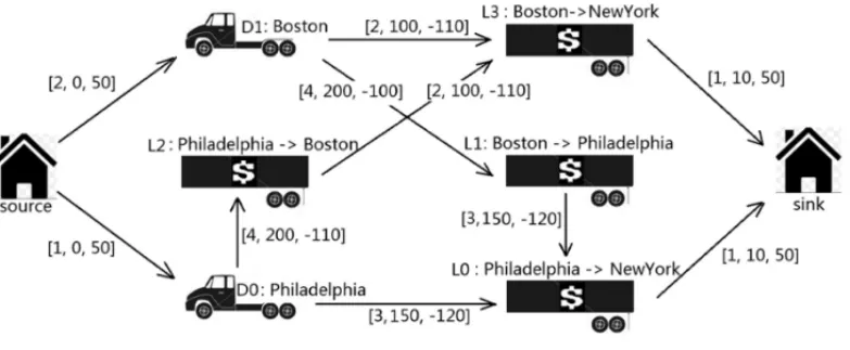
j ,C′j). IfB(O)=∅, return toStep 2; otherwise return toStep 3. A simple graph with two resource constraints (time, distance) and cost is presented in Figure 2 and Table 1, followed by an example to show how the algorithm works. Figure 2 shows the node and link connections in the network. Table 1(a) shows the drivers’ profile. Table 1(b) shows loads’ profile. Table 1(c) shows the constraint for the drivers and loads. In this example, the constraints are time window and mileage. Table 1(d) shows the resources being consumed on each link, as well as the cost on each link. Note that the actual route, which has multiple links, can be 14-days long and undertake more than just two or three loads.
Figure 2– Subproblem Network.
Wherea0andb0are the beginning and ending pick-up times, anda1andb1are the minimum
Tables 1a-1d– Sample Database Tables.
Deadhead is typically discouraged because moving an empty truck comes with a cost but there is no (direct) gain in revenue. Simply speaking, driverD0is originally located at Philadelphia
and is eligible for Load L0andL2at the beginning. Once the load is delivered, the driver may
become available again at the load destination (New York or Boston, depending on the load). Preprocessor skips the ineligible connections and adds eligible connections in term of links to the network. This preprocessing is a necessary step to reduce the problem size of the subproblem.
Step 1. Initialization.
PS=QS=(0,0,0),PD0= PD1=PL0= PL1= PL2=PL3= PT =∅,
QD0 = (7,0,−∞), QD1 = (7,0,−∞), QL0 = (8,0,−∞), QL1 = (7,0,−∞), QL2=(7,0,−∞),QL3=(8,0,−∞),QT =(12,0,−∞),
dD0 = (2,0,50), dD1 = (1,0,50), dL0 = (2,100,−110), dL1 = (4,200,−110), dL2=(4,200,−100),dL3=(3,150,−120),dT =(1,10,50), and
O= {(7,0,−∞)D0, (7,0,−∞)D1, (7,0,−∞)L1, (7,0,−∞)L2, (8,0,−∞)L0, (8,0,−∞)L3,
(12,0,−∞)T}.
Step 2. F(O)=(7,0,−∞)D0.
Step 3. B(O) = (Dk∗,Ck)∈ O|(7,0,−∞)≤L(D∗k,Ck)<L(9,0,−∞)
. We treat label(7,0− ∞).
Step 5. Replacement of(7,0,−∞). (A) RD0 = R PD0 = (7,0,50); (C) PD0 = QD0 =
(7,0,50). O = {(7,0,−∞)D1, (7,0,−∞)L1, (8,0,−∞)L2, (8,0,−∞)L0, (8,0,−∞)L3,
(12,0,−∞)T}. We treat label(7,0− ∞).
Step 4. Uncertainty zoneT RD1=(8,500).
Step 5. Replacement of(7,0,−∞). (A) RD1 = R PD1 = (7,0,50); (C) PD1 = QD1 =
(7,0,50). O = {(7,0,−∞)L1, (7,0,−∞)L2, (8,0,−∞)L0, (8,0,−∞)L3, (12,0,−∞)T}, We treat label(7,0− ∞).
Step 4. Uncertainty zoneT RL1=(12,500).
Step 5. Replacement of(7,0,−∞). (A)RL1 = R PL1 =(11,200,−60); (C)PL1 = QL1 =
(11,200,−60). O = {(7,0,−∞)L2, (8,0,−∞)L0, (8,0,−∞)L3, (12,0,−∞)T}, We treat label(7,0− ∞).
Step 4. Uncertainty zoneT RL2=(12,500).
Step 5. Replacement of(7,0,−∞). (A)RL2 = R PL2 =(11,200,−50); (C)PL2 = QL2 =
(11,200,−50).O= {(8,0,−∞)L0, (8,0,−∞)L3, (12,0,−∞)T}, We treat label(8,0− ∞).
Step 4. Uncertainty zoneT RL0=(18,500).
Step 5. Replacement of(8,0,−∞). (A)RL0=R PL0= {(9,100,−60), (13,300,−170)}; (C) PL0=QL0= {(9,100,−60), (13,300,−170)}.O= {(8,0,−∞)L3, (12,0,−∞)T}, We treat label(8,0− ∞).
Step 4. Uncertainty zoneT RL3=(18,500).
Step 5. Replacement of(8,0,−∞). (A) RL3 = R PL3 = {(10,150,−70), (14,350,−170)};
(C) PL3 = QL3 = {(10,150,−70), (14,350,−170)}. O = {(12,0,−∞)T}, We treat label
(12,0− ∞).
Step 4. Uncertainty zoneT RT =(18,500).
Step 5. Replacement of(12,0,−∞). (A) RT = R PT = {(10,110,−10), (11,160,−20),
(14,310,−120), (15,360,−120); (C) PT = QT = {(10,110,−10), (11,160,−20),
(14,310,−120),(15,360,−120).
Step 2. O = ∅. Stop. Current solution{(10,110,−10), (11,160,−20), (14,310,−120), (15,360,−120)}. There are four shortest paths from the source nodeS to the sink node T re-specting the resource constraints: (1) Path: S → D0 → L0 → T with cost−10; (2) Path:
Path 4 is dominated by Path 3. As a result, Paths 1, 2 and 3 are non-dominated optimal and are eligible to be added into the path/route pools in the master problem.
Note that in this example, labels in P and Q are always having the same sets of labels and paths because the resource constraints never get violated. In the case where certain paths exceed the resource limit, those parts are deemed as infeasible and therefore excluded at the current stage. The lower boundQ, however, would keep this infeasible label for future treatments. This technique is extremely useful when the resource on a directed link is negative. In other words, the previously infeasible path may become feasible again by adding consecutive links to it. This means that before all the paths are examined, one simply cannot determine the best or even most feasible paths.
6 THE SCHEME OF BRANCH AND BOUND (B&B)
Commercial software CPLEX is used to solve the master problem (linear programming relax-ation). The optimal solution is generally non-integer (fractional). The B&B scheme is thus in-voked and embedded into the column generation process to obtain an integer solution. The fol-lowing are the details for the implementation (refer to the flow chart). If there is any existing feasible solution can be extracted from the current truck operating plan, then it should be utilized as the initial solution to speed up the search process.
6.1 The Branching Strategy
It is easy to observe that if the solution is non-integer, there must exist at least a pair of consecu-tive load nodest1,t2such that
0< xj j∈T R(t1,t2)
<1,
whereT R(t1,t2)is the set of routes in whicht2is executed immediately aftert1. Based on the setT R(t1,t2), the original problem is partitioned (branched) into two subproblems:
0-branch, xj j∈T R(t1,t2)
=0, 1-branch, xj j∈T R(t1,t2)
=1.
The testing shows that this strategy gives a more balanced search tree than default variable branching and generally finds an acceptable integer solution more quickly. Conceivably, this method is to branch on the relationship between two consecutive loads. It forces the link to be selected or to be eliminated in the subproblem.
6.2 How B&B Scheme is Embedded into the Column Generation Process?
– one with xj j∈T R(t1,t2)
=0 (left node),
– and the other with xj j∈T R(t1,t2)
=1 (right node).
Bycreating a node we mean that the objective value and the solution at the node are found. Only the node corresponding to fractional solution with objective value smaller than that of the current optimal integer solution is inserted into the queue. Once a node corresponding to an integer solution is created and its objective value is smaller than that of the current optimal integer solution, then all untreated nodes in the queue with objective value not smaller than that of the created node will be pruned off. Whenever a node a created, a set of columns (for solving the master problem) and a network (for solving the subproblem) should be updated accordingly.
6.3 Information Storage and Retrieval
For solving the master problem and the subproblem at different nodes of the search tree, the information on columns and network must conform to the node to be created. There are two ways to get the information: one is from the root node; the other is from the node to be treated (parent node). With the first one, much more memory can be saved, but more computing time is needed (repeated computing), while with the second, the situation is reversed. There is a trade-off between the memory and the computing time. In the first case, we only need to store the original network and the columns generated at root node. The search tree is a binary tree and the root node is at 0 level. We use a label consisting of(j +1)identifiers to represent the location of a node at j-th level: (j,j1,j2, . . . ,jj), where the first onej is a digit (or digits) which represents the level number of the node location; the second one j1represents the location (left or right)
of its ancestor at the first level; the third one j2represents the location of its ancestor at second
level,. . . , and jj represents its location at j-th level. j1,j2, . . . , jj = L or R, L stands for left branch (0-branch); R stands for right branch (1-branch). For example, a node with label
(3,R,R,L)means that the node is at the third level of the search tree, and its ancestors are at the first and second levels on the right location. The third-level node is at left location. In the second case, we only need to indicate where the treated node is located and then modify the columns and network of its parent node respectively to process.
6.4 The Modification of the Columns for the Master Problem
In the 0-branch, we delete all columnsifor whichat1,i =1 andat2,i =1. In the 1-branch, we
delete all columnsi for whichat1,i = 1 andat2,i =0, orat1,i =0 andat2,i =1, and the row
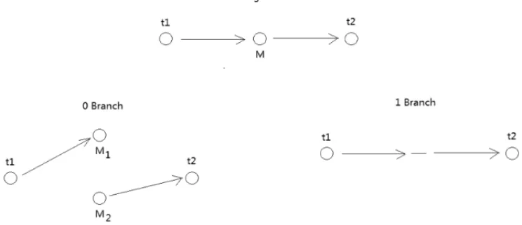
corresponding to constraint for nodet2due to the redundancy. Figure 3 illustrates this process. The underlying assumption is that each load can be covered only once at most. The 2nd coverage for the same load will not bring additional revenue.
Figure 3– Sample Branching.
where the information is obtained. For example, if we use the information on columns at root node and the created nodes are(3,R,R,L), then all columns at root node havingat1,i =1 and at2,i = 0, at1,i = 0 andat2,i = 1,at3,i = 1 andat4,i = 0,at3,i = 0 andat4,i =1,at5,i = 1
andat6,i = 1 are deleted. The row corresponding to constraint for nodet6is also deleted due
to the redundancy. We assume that the branching at first, second, and third level is based on
T R(t1,t2),T R(t3,t4),T R(t5,t6)respectively.
6.5 Modification of the Network for the Subproblem
We must restrict the columns to be generated by the subproblem to those that are compatible with the current created node in the search tree. The structure of the network used to generate the feasible columns should be modified accordingly. In the 0-branch, the columns covering consec-utively nodest1andt2are forbidden. As a reminder, there are the columns havingt2executed immediately aftert1. In the network we split the middle node M, where the link corresponding
tot1terminates and the link corresponding tot2starts, into two nodesM1andM2; all links
orig-inally terminated atM are now moved toM1, and all links originally started fromM are moved
toM2. The resource constraints onM1andM2remain the same asM. In the 1-branch, we force
any route coveringt1to also covert2immediately. In the network, the two links corresponding tot1andt2are condensed into one link, and all the links originally terminated at the middle node
+ cost(t2), where cost(t1) and cost(t2) are the cost oft1andt2, respectively; (b) the number of
pieces of work still equals zero ; (c) the spread equalst1+t2; (d) the work time equalst1+t2.
Figure 4– Sample Network Modification.
With the same example, for the created node(3,R,R,L)the modified network at this node is obtained from the original network. After splitting the two nodes (one between the links corre-sponding tot1andt2, and the other betweent3andt4) into four nodes, and condensing two links
corresponding tot5andt6into one, all the links originally terminated at the middle node of the links corresponding tot5andt6are deleted.
In the iteration process, a set of the dual values are passed from master problem. The cost(ti)of the linkicorresponding to load nodeti (i-th constraint) is subtracted by dual valueπbefore the subproblem algorithm is executed. Once the desirable columns are generated, the cost of each linki is set to cost(ti)(the original cost).
6.6 The Order of Choosing the Next Node and the Queue
The sum of fractional variables for a specified set T R(t1,t2)and the objective values at each node should determine the next node to branch on. The node with smallest sum of fractions is chosen as a priority. If there is a tie, the one with the smaller objective value is chosen. If there is still a tie, then choose any arbitrary one. One should always keep a sorting queue (non-decreasing sequence of the sum of fractional variables) for the nodes to be treated and take the first one from the queue. When a fractional solution occurs, and its objective value is smaller than that of current optimal integer solution value, then the node corresponding to this frac-tional solution is inserted into the queue. Before inserting, we need to know the sum of fractions. From the fractional solution, one must find the first columnxi <1 and a setT R(t1,t2)consisting of two consecutive nodest1andt2in columnxi such that
0< xj j∈T R(t1,t2)
<1;
7 TESTING RESULTS AND REMARKS
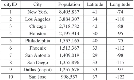
To prove the capability of the prototyped routing optimizer, we select top 10 US cities with the largest populations and set Dallas as home based depot (as shown in Table 2 and Figure 5).
Table 2– Top 10 US Cities with the Largest Populations.
cityID City Population Latitude Longitude
1 New York 8,405,837 41 -74
2 Los Angeles 3,884,307 34 -118
3 Chicago 2,718,782 42 -88
4 Houston 2,195,914 30 -95
5 Philadelphia 1,553,165 40 -75
6 Phoenix 1,513,367 33 -112
7 San Antonio 1,409,019 29 -98
8 San Diego 1,355,896 33 -117
9 Dallas (depot) 1,257,676 33 -97
10 San Jose 998,537 37 -122
Figure 5– Top 10 US Cities with the Largest Populations.
From these 10 cities we can have 45 non-directional city pairs sorted in an alphabet order on the origin city and destination city (as shown in Table 3).
Table 3– Forty-Five Non-directional City-Pairs.
odID Orig Dest Miles odID Orig Dest Miles
1 Chicago Dallas 967 24 Houston San Jose 1885
2 Chicago Houston 1083 25 Los Angeles New York 2778
3 Chicago Los Angeles 2016 26 Los Angeles Philadelphia 2710
4 Chicago New York 791 27 Los Angeles Phoenix 373
5 Chicago Philadelphia 758 28 Los Angeles San Antonio 1353
6 Chicago Phoenix 1735 29 Los Angeles San Diego 120
7 Chicago San Antonio 1242 30 Los Angeles San Jose 341
8 Chicago San Diego 2139 31 New York Philadelphia 97
9 Chicago San Jose 2163 32 New York Phoenix 2409
10 Dallas Houston 967 33 New York San Antonio 1821
11 Dallas Los Angeles 1436 34 New York San Diego 2799
12 Dallas New York 1547 35 New York San Jose 2944
13 Dallas Philadelphia 1467 36 Philadelphia Phoenix 2344
14 Dallas Phoenix 1065 37 Philadelphia San Antonio 1742
15 Dallas San Antonio 274 38 Philadelphia San Diego 2735
16 Dallas San Diego 1358 39 Philadelphia San Jose 2911
17 Dallas San Jose 1687 40 Phoenix San Antonio 981
18 Houston Los Angeles 1548 41 Phoenix San Diego 355
19 Houston New York 1627 42 Phoenix San Jose 711
20 Houston Philadelphia 1548 43 San Antonio San Diego 1276
21 Houston Phoenix 1174 44 San Antonio San Jose 1692
22 Houston San Antonio 197 45 San Diego San Jose 460
23 Houston San Diego 1468
One of the performance measurements is Load Factor (LF). For each truck driver route, LF is the total loaded miles divide by total miles (loaded miles + empty miles) traveled starting from and returning to the depot: Dallas.
100 random generated data sets have been tested between current existing algorithm and our new column-generation based algorithm to compare both number of drivers used and Load Factor (LF) to complete each set of 45 loads crossing those 10 cities. Table 4 gives the details on each test case. The average run time is very stable and is within a few minutes for the tested problem size. Table 5 shows the overall performance.
Our sample testing indicates that our new column-generation based solution method will reduce about 16% of drivers and improve the Load Factor (LF) by about 9%.
Table 4– Computational Results of 100 Tests.
testID Existing Method New Method Driver LF num drivers LF num drivers LF Reduced (%) Improved (%)
1 18 63 15 70 20 11.1
2 16 69 14 73 14.3 5.8
3 15 70 14 73 7.1 4.3
4 17 66 15 71 13.3 7.6
5 17 68 14 74 21.4 8.8
6 19 62 16 66 18.8 6.5
7 18 63 16 68 12.5 7.9
8 18 62 15 69 20 11.3
9 16 69 14 75 14.3 8.7
10 18 62 16 68 12.5 9.7
11 19 58 17 66 11.8 13.8
12 17 68 14 76 21.4 11.8
13 17 65 15 72 13.3 10.8
14 17 65 16 67 6.3 3.1
15 17 67 15 72 13.3 7.5
16 16 69 13 79 23.1 14.5
17 18 61 14 73 28.6 19.7
18 17 66 15 71 13.3 7.6
19 18 62 16 65 12.5 4.8
20 19 59 17 63 11.8 6.8
21 17 67 15 69 13.3 3
22 17 66 15 72 13.3 9.1
23 17 65 14 75 21.4 15.4
24 17 65 15 69 13.3 6.2
25 16 71 14 74 14.3 4.2
26 19 58 16 66 18.8 13.8
27 17 69 14 77 21.4 11.6
28 17 66 15 74 13.3 12.1
29 17 65 15 73 13.3 12.3
30 16 69 15 71 6.7 2.9
31 18 63 14 75 28.6 19
32 17 65 14 74 21.4 13.8
33 18 61 15 68 20 11.5
34 18 61 15 69 20 13.1
35 16 72 14 73 14.3 1.4
36 18 64 16 68 12.5 6.3
37 18 61 16 66 12.5 8.2
38 18 64 16 67 12.5 4.7
39 17 65 15 71 13.3 9.2
40 17 63 16 67 6.3 6.3
41 16 68 14 76 14.3 11.8
Table 4 (continuation).
testID Existing Method New Method Driver LF num drivers LF num drivers LF Reduced (%) Improved (%)
43 17 68 14 77 21.4 13.2
44 17 68 14 72 21.4 5.9
45 16 69 13 76 23.1 10.1
46 16 71 14 74 14.3 4.2
47 18 62 15 71 20 14.5
48 16 69 15 69 6.7 0
49 17 65 13 77 30.8 18.5
50 17 66 14 72 21.4 9.1
51 18 64 16 68 12.5 6.3
52 17 68 14 73 21.4 7.4
53 18 59 17 62 5.9 5.1
54 17 63 16 64 6.3 1.6
55 19 60 17 63 11.8 5
56 17 65 14 72 21.4 10.8
57 17 67 14 74 21.4 10.4
58 19 62 16 66 18.8 6.5
59 18 64 16 67 12.5 4.7
60 18 63 15 68 20 7.9
61 17 64 15 70 13.3 9.4
62 18 62 15 69 20 11.3
63 17 65 15 70 13.3 7.7
64 18 61 14 73 28.6 19.7
65 17 64 15 71 13.3 10.9
66 19 58 18 59 5.6 1.7
67 17 68 14 76 21.4 11.8
68 18 64 14 73 28.6 14.1
69 16 71 13 78 23.1 9.9
70 17 64 13 79 30.8 23.4
71 19 61 17 64 11.8 4.9
72 17 68 14 75 21.4 10.3
73 18 63 15 70 20 11.1
74 18 60 18 60 0 0
75 17 65 14 74 21.4 13.8
76 17 68 15 72 13.3 5.9
77 17 63 16 65 6.3 3.2
78 18 65 15 71 20 9.2
79 17 69 13 80 30.8 15.9
80 17 66 13 77 30.8 16.7
81 16 70 15 71 6.7 1.4
82 18 66 15 71 20 7.6
83 18 62 14 72 28.6 16.1
Table 4 (continuation).
testID Existing Method New Method Driver LF num drivers LF num drivers LF Reduced (%) Improved (%)
85 18 64 15 71 20 10.9
86 17 65 15 71 13.3 9.2
87 16 67 15 73 6.7 9
88 16 71 14 73 14.3 2.8
89 18 65 13 78 38.5 20
90 16 70 16 67 0 -4.3
91 17 63 14 74 21.4 17.5
92 17 68 15 70 13.3 2.9
93 17 64 15 71 13.3 10.9
94 17 66 14 76 21.4 15.2
95 17 65 14 73 21.4 12.3
96 19 60 17 64 11.8 6.7
97 17 66 14 72 21.4 9.1
98 19 60 17 64 11.8 6.7
99 18 62 15 70 20 12.9
100 17 67 14 73 21.4 9
Table 5– Comparison Between Existing And New Methods.
Existing Method New Method Driver LF
avg drivers avg LF avg drivers avg LF Reduced (%) Improved (%)
17.3 65 14.9 70.9 16.3 9.1
decision variable is defined as a route, which is the combination of drivers, the loads and se-quence of covering the loads. Without any of the preprocessing to eliminate routes, the number of decision variables is 2.5×10²⁰ if the maximum of four loads are allowed in a single route. This number increases to 3.8×1024 if five loads are allowed in a single route. The prototype successfully considered all the major business criteria and constraints to have problem solved within 20 minutes on the company’s mainframe machine. After comparing with the company’s then-current operating plan, over 10% cost saving was achieved, which amounted to millions of dollars annually.
REFERENCES
[1] BASTIAN C & RINNOOYKAN AHG. 1992. The Stochastic Vehicle Routing Problem Revisited.
European Journal of Operational Research,56: 407–412.
[2] BERMANO & SIMCHI-LEVID. 1989. The Traveling Salesman Location Problem on Stochastic Networks.Transportation Science,23: 54–57.
[3] BERTSIMASDJ & HOWELL LH. 1993. Further Results on the Probabilistic Traveling Salesman Problem.European Journal of Operational Research,65: 68–95.
[4] BRAEKERSK, RAMAEKERSK & VAN NIEUWENHUYSEI. 2016. The vehicle routing problem: State of the art classification and review.Computers & Industrial Engineering,99: 300–313.
[5] BRAMELJ, COFFMANJREG, SHORP & SIMCHI-LEVID. 1992. Probabilistic Analysis of Algo-rithms for the Capacitated Vehicle Routing Problem with Unsplit Demands.Operations Research,40: 1095–1106.
[6] BRAMELJ, LICL & SIMCHI-LEVID. 1994. Probabilistic Analysis of the Vehicle Routing Problem with Time Windows.American Journal of Mathematical and Management Science,13: 267–322.
[7] COOKTM & RUSSELLRA. 1978. A Simulation and Statistical Analysis of Stochastic Vehicle Rout-ing with TimRout-ing Constraints.Decision Science,9: 673–687.
[8] DERIGSU, PULLMANNM & VOGELU. 2013. Truck and Trailer Routing-Problems, Heuristics and Computational Experience.Computers and Operations Research,40: 536–546.
[9] DESROCHERSM, LENSTRAJK & SAVELSBERGHMWP. 1990. A Classification Scheme for Vehicle Routing and Scheduling Problems.European Journal of Operational Research,46: 322–332.
[10] GOLDENBL & STEWARTWR. 1978. Vehicle Routing with Probabilistic Demands. HOGBEND & FIFED. (eds.).Computer Science and Statistics: Tenth Annual Symposium on the Interface. NBSS Special Publication, National Book Service, Toronto, Canada, pp. 252–259.
[11] LABADIEN & PRINSC. 2012. Vehicle Routing Nowadays: Compact Review and Emerging Prob-lems. In:Production System and Supply Chain Management in Emerging Countries: Best Practices, Selected Papers From the International Conference on Production Research (ICPR). Springer, Berlin, pp. 141–166.
[12] LAPORTEG, LOUVEAUXFV & MERCUREH. 1994. A Priori Optimization of the Probabilistic Traveling Salesman Problem.Operations Research,42: 543–549.
[13] LAPORTEG, TOTHP & VIGOD. 2013. Vehicle Routing: Historical Perspective and Recent Contri-butions.European Journal of Operational Research,1: 1–4.
[14] LIY, MIAOQ & WANGX. 2014. High-Speed Train Network Routing with Column Generation.
Transportation Research Record: Journal of the Transportation Research Board,2466: 58–67.
[15] LI Y, MIAO Q & WANG X. 2010. A Column Generation Method for the U.S. Army Logistics Air Fleet Scheduling. In:Transportation Research Record: Journal of the Transportation Research Board,2197: 36–42.
[17] POWELL WB, JAILLET P & ODONIA. 1995. Stochastic and Dynamic Networks and Routing. BALLMO, MAGNANTITL, MONMACL & NEMHAUSERGL. (eds.).Handbooks in Operations Research and Management Science, 8. Network Routing. Elsevier (North-Holland), Amsterdam, pp. 141–296.
[18] POWELLWB, SNOWW & CHEUNGRK. 2000. Adaptive Labeling Algorithms for the Dynamic Assignment Problem.Transportation Science,34: 50–66.
[19] SOLOMON MM. 1987. Algorithms for the Vehicle Routing and Scheduling Problem with Time Window Constraints.Operations Research,35: 254–265.
[20] STEWART WR & GOLDEN BL. 1983. Stochastic Vehicle Routing: A Comprehensive Approach.
European Journal of Operational Research,14: 371–385.
[21] YANG J, JAILLET P & MAHMASSANIH. 2004. Real-Time Multivehicle Truckload Pickup and Delivery Problems.Transportation Science,38(2): 135–148.